Shape invariant potentials in SUSY quantum mechanics and periodic orbit theory

Abstract

We examine shape invariant potentials (excluding those that are obtained by scaling) in supersymmetric quantum mechanics from the stand-point of periodic orbit theory. An exact trace formula for the quantum spectra of such potentials is derived. Based on this result, and Barclay’s functional relationship for such potentials, we present a new derivation of the result that the lowest order SWKB quantisation rule is exact.

In non-relativistic quantum mechanics certain potentials are amenable to exact analytic solution. For a subset of these soluble potentials, the energy spectrum may be expressed explicitly as an algebraic function of a single quantum number. Such potentials occur either in one space dimension, or are central potentials in higher dimensions. For the latter, an effective potential in the radial variable can be defined for each partial wave. Some examples of such potentials are Coulomb, harmonic oscillator, Morse, Rosen-Morse, etc. cooper1 . These potentials also have the property that the lowest order WKB quantisation rule, together with the appropriate Maslov index (that may change from potential to potential migdal ) , leads to exact results. For central potentials, the Langer prescription langer for the centrifugal barrier, together with half-integer quantisation, can also be employed barclay .

In supersymmetric (SUSY) quantum mechanics, these exactly solvable potentials are found to be translationally shape invariant gend . Combining SUSY and WKB, Comtet et al. comtet found that the lowest order SWKB calculation needs neither the Maslov index nor the Langer correction to yield the exact result. The purpose of the present paper is to understand this result from the point of view of the periodic orbit theory (POT) brack , rather than the higher order WKB corrections khare . Regarding the latter, we should point out a largely overlooked paper by Barclay barclay , in which he showed that the higher order WKB terms converge in these potentials to yield an energy-independent correction. The latter may be absorbed in the Maslov index of the lowest order term. For SWKB, all the higher order terms vanish. Although we do not make the WKB expansion, we arrive at the same result in a novel application of POT.

We first set the notation by reviewing the relevant equations of SUSY QM. Consider a potential $V(x;a_{1})$ of a single variable $x$, and a set of parameters denoted by $a_{1}$. One defines a “super potential”

$$W(x;a_{1})=-{\hbar\over{\sqrt{2m}}}{\phi^{\prime}_{0}(x)\over{\phi_{0}(x)}}~{},$$

where $\phi_{0}(x)$ is the ground state solution of the Schrödinger equation at energy $E_{0}$ for the potential $V(x,a_{1})$, and a prime denotes the spatial derivative. Let us define

$$V_{1}(x;a_{1})=(V(x;a_{1})-E_{0})~{},$$ (1)

so that the ground state energy of the Hamiltonian

$$H_{1}=-{\hbar^{2}\over{2m}}{d^{2}\over{dx^{2}}}+V_{1}(x;a_{1})$$

lies at zero energy, i.e., $E_{0}^{(1)}=0$. Then it is easy to show that

$$V_{1}(x;a_{1})=W^{2}(x;a_{1})-{\hbar\over{\sqrt{2m}}}W^{\prime}(x;a_{1})~{}.$$

The SUSY partner Hamiltonian $H_{2}$ has the potential $V_{2}(x;a_{1})$, and has an energy spectrum identical to that of $H_{1}$, except for the absence of the zero-energy state. The ground state of $H_{2}$, denoted by $E_{0}^{(2)}$ coincides with the first excited state $E_{1}^{(1)}$ of $H_{1}$, and so on. The partner potential $V_{2}(x;a_{1})$ is

$$V_{2}(x;a_{1})=W^{2}(x;a_{1})+{\hbar\over{\sqrt{2m}}}W^{\prime}(x;a_{1})~{}.$$

Shape invariance in the partner potentials is defined by the relation

$$V_{2}(x;a_{1})=V_{1}(x;a_{2})+R(a_{1})~{},$$ (2)

where the new parameters $a_{2}$ are some function of $a_{1}$, and the remainder $R(a_{1})$ is independent of the variable $x$. We restrict our consideration of shape invariance to those cases where $a_{2}$ and $a_{1}$ are related by translation, $a_{2}=a_{1}+\alpha$. It is then straight forward to show, by constructing a hierarchy of Hamiltonians that the complete eigenvalue spectrum of $H_{1}$ is given by cooper1

$$E_{n}^{(1)} = \sum_{k=1}^{n}R(a_{k})~{},~{}~{}n\geq 1~{},$$ (3)

$$E_{0}^{(1)} = 0~{}.$$ (4)

The RHS of the above may be expressed as a monotonic function $f_{1}(n)$ of the quantum number $n$, so that

$$E_{n}^{(1)}=f_{1}(n)~{};~{}~{}~{}~{}f_{1}(0)=0~{}.$$ (5)

For the shape invariant potentials we consider here, $f_{1}(n)$ is an algebraic function. Using this property, we proceed to obtain an exact expression for the quantum density of states of $H_{1}$ in the spirit of periodic orbit theory. This entails a division of the density of states into a smooth and an oscillating part as a function of a continuous classical variable $E$. To this end, we may write

$$\delta(E-E_{n}^{(1)})=\delta(E-f_{1}(n))=\delta(n-F_{1}(E))F_{1}^{\prime}(E),$$ (6)

where the relation $E=f_{1}(n)$ has been inverted to define

$$n=F_{1}(E)~{}.$$ (7)

(When the mapping between $n$ and $E_{n}$ is $(1,1)$ there is no difficulty in the inversion. But to define the derivative $F_{1}^{\prime}(E)$ requires an extension from the discrete to the continuum, and that is not unique. In the case of shape invariant potentials we have an algebraic relation which solves that problem.) For the spectrum under consideration, $f_{1}(0)=0$ implies the condition

$$F_{1}(0)=0~{}.$$ (8)

The quantum density of states $g_{1}(E)$ for the discrete spectrum of $H_{1}$ is defined as

$$g_{1}(E)=\sum_{n=0}^{\infty}d(n)\delta(E-E_{n}^{(1)})~{},$$ (9)

where $d(n)$ is the degeneracy of states at $E=E_{n}$. Writing $d(n)=d(F_{1}(E))=D(E)$, and using Eq. (6), we obtain

$$g_{1}(E)=D(E)F_{1}^{\prime}(E)\sum_{n=0}^{\infty}\delta(n-F_{1}(E))~{}.$$ (10)

($D(E)=1$ for one-dimensional potentials). We now use the identity

$$\sum_{n=0}^{\infty}\delta(n-x)=\sum_{k=-\infty}^{\infty}e^{2i\pi kx}~{},~{}~{}x\geq 0~{},$$ (11)

to obtain the desired expression brack ; jennings

$$g_{1}(E)=D(E)F_{1}^{\prime}(E)\left[1+2\sum_{k=1}^{\infty}\cos[2\pi kF_{1}(E)]\right]~{}.$$ (12)

For a given $F_{1}(E)$, this is an exact expression for the quantum density of states $g_{1}(E)$. It is in the form of a trace formula in POT brack ; Balian when $F_{1}(E)$ (to within a dimensionless additive constant $\eta$) is related to the action $S_{1}(E)$ of the primitive classical periodic orbit of the potential $V_{1}(x)$ :

$${S_{1}(E)\over h} = F_{1}(E)+\eta~{},$$ (13)

$$S_{1}(E) = 2\sqrt{2m}\int_{x_{1}}^{x_{2}}\sqrt{E-V_{1}}~{}dx~{}.$$ (14)

In the above, $x_{1}$ and $x_{2}$ are the classical turning points at which $E=V_{1}(x)$ (for simplicity in notation, we write $V_{1}(x,a_{1})=V_{1}(x)$). The ($h-$independent constant) $\eta$ may be determined by using Eq. (13), and applying the condition given by Eq. (8) for $E=0$. We then obtain

$$\eta={S_{1}(0)\over h}~{}.$$ (15)

We may prove Eq. (13) by noting that the (smooth) Thomas-Fermi density of states, given by the first term on the RHS of Eq. (12), is the Laplace inverse of the classical canonical partition function ross of the Hamiltonian $H_{1}^{cl}(x,p)=p^{2}/2m+V_{1}(x)$ :

$$F_{1}^{\prime}(E)={\cal{L}}^{-1}_{E}~{}Z_{1}^{cl}(\beta)~{}~{}={1\over{2\pi i}}\int_{c-i\infty}^{c+i\infty}Z_{1}^{cl}(\beta)e^{\beta E}~{}d\beta.$$ (16)

Since

$$Z_{1}^{cl}(\beta) = {1\over h}\int\exp[-\beta\,H_{1}^{cl}(x,p)]~{}dxdp$$ (17)

$$= {1\over{2\pi\hbar}}\sqrt{2m\pi\over\beta}\int_{-\infty}^{\infty}\exp[-\beta V_{1}(x)]dx~{},$$

it follows from (16) that

$$F_{1}^{\prime}(E)={\sqrt{2m}\over{2\pi\hbar}}\int_{x_{1}}^{x_{2}}{dx\over{\sqrt{[E-V_{1}(x)]}}}~{}.$$ (18)

From this, Eq. (13) follows on integration over energy. Using Eq. (7) together with (13, 14), we obtain the important result that the lowest order WKB quantisation rule is exact for $V_{1}$ :

$$S_{1}(E)=\oint p(x)dx=(n+\eta)h~{},$$ (19)

where $p(x)=\sqrt{2m[E-V_{1}(x)]}$. We also see that the constant $\eta$ is the so called Maslov index which may vary from one potential to the other.

The Maslov index $\eta$ may be eliminated from the quantisation rule by employing the superpotential formalism, and the result of Barclay and Maxwell barcmax . They made the important observation that the shape invariant class of potentials under consideration obey one or other of the following equations:
Class I

$$\frac{\hbar}{\sqrt{2m}}{dW\over dx}=A+BW^{2}(x)+CW(x)~{},$$ (20)

or Class II

$$\frac{\hbar}{\sqrt{2m}}{dW\over dx}=A+BW^{2}(x)+CW(x)\sqrt{(A+BW^{2})}~{},$$ (21)

where A, B and C are constants. Using these equations, we now show that $S_{1}(E)$, as defined by Eq. (14), obeys the relation ($x_{1s}$, $x_{2s}$ are the turning points in SWKB)

$$S_{1}(E)=2\sqrt{2m}\int_{x_{1s}}^{x_{2s}}\sqrt{E-W^{2}}~{}dx~{}+h\eta~{}.$$ (22)

To this end, note that the action $S_{1}$ can be expressed as an inverse Laplace transform

$$S_{1}(E)=\sqrt{2m\pi}~{}{\cal L}^{-1}_{E}\int_{-\infty}^{\infty}{e^{-\beta[W^{2}-\hbar W^{\prime}/\sqrt{2m}]}\over{\beta^{3/2}}}dx~{}.$$ (23)

At this point, for simplicity of notation, let us temporarily put $\hbar/\sqrt{2m}=\gamma$. Expanding the exponential in powers of $W^{\prime}$, we have

$$S_{1}(E)=$$ (25)

$$\sqrt{2m\pi}{\cal L}^{-1}_{E}\int_{-\infty}^{\infty}{e^{-\beta W^{2}}\over{\beta^{3/2}}}\left(1+\sum_{k=0}^{\infty}{(\gamma\beta W^{\prime})^{k+1}\over{(k+1)!}}\right)~{}dx~{}.~{}$$

$$= 2\sqrt{2m}\int_{x_{1s}}^{x_{2s}}\sqrt{E-W^{2}}dx+$$

$$\quad\sum_{k=0}^{\infty}{\hbar\over(k+1)!}{\partial^{k}\over\partial E^{k}}\int_{-\sqrt{E}}^{\sqrt{E}}{(\gamma W^{\prime})^{k}\over{\sqrt{E-W^{2}}}}dW~{}.$$

Note that now the limits in $x$ are replaced by the condition $W^{2}(x)=E$. The integral for $k=0$ may be done immediately, yielding $\pi$. To evaluate the integrals for integer $k\geq 1$, we assume that $\gamma\,W^{\prime}$ obeys Barclay’s equation (20) (class I) or (21) (class II).

For class I, we require integrals of the type

$$I_{k}=\int_{-\sqrt{E}}^{\sqrt{E}}{(A+BW^{2}+CW)^{k}\over\sqrt{E-W^{2}}}dW~{}.$$ (26)

On expanding the numerator, terms with odd powers of $W$ vanish on integration. One now sees that only the piece of $I_{k}$ involving the highest power of $W^{2}$ survives the differentiation in Eq. (25). Consider the integral with $W^{2k}$. With the substitution $W=\sqrt{E}\sin\theta$

$$\int_{-\sqrt{E}}^{\sqrt{E}}{W^{2k}\over\sqrt{E-W^{2}}}dW = E^{k}\int_{-\pi/2}^{\pi/2}\rm{sin}^{2k}\theta d\theta~{}$$ (27)

$$= E^{k}{(2k-1)!!\over{(2k)!!}}\pi~{}.$$ (28)

Accordingly, Eq. (25) reduces to

$$S_{1}(E) = 2\sqrt{2m}\int_{x_{1s}}^{x_{2s}}\sqrt{E-W^{2}}dx\,\,+$$ (29)

$$\quad\hbar\pi\left(1+\sum_{k=1}^{\infty}{B^{k}(2k-1)!!\over{(k+1)(2k)!!}}\right)~{}.$$

By construction, $W^{2}(x)$ has coincident turning points at $E=0$, so the first term on the RHS above vanishes at this energy. Comparing with Eq. (15), we deduce that

$$\eta = {1\over 2}\left(1+\sum_{k=1}^{\infty}{B^{k}(2k-1)!!\over{(k+1)(2k)!!}}\right)$$ (30)

$$= \frac{1}{B}[1-\sqrt{1-B}]~{}.$$

Note, from Eq. (20), that $B$ is independent of Planck’s constant $h$. Comparing now with Eq. (13), we deduce our main result

$$2\pi\hbar F_{1}(E)=\sqrt{2m}\oint~{}\sqrt{E-W^{2}}dx~{}.$$ (31)

Using Eq. (7) we get as the exact result the SWKB expression

$$\oint~{}\sqrt{2m(E-W^{2})}dx~{}=2\pi\hbar n~{},~{}~{}n=0,1,2,3,\cdots$$ (32)

which yields the quantum spectrum of $V_{1}(x)$.

A similar derivation may be carried through for class II superpotentials obeying Eq. (21). The starting point, as before, is Eq. (25), and the integral to be considered is now of the form

$$J_{k}=\int_{-\sqrt{E}}^{\sqrt{E}}{(A+BW^{2})^{k}\left(1+{CW\over{\sqrt{A+BW^{2}}}}\right)^{k}\over{\sqrt{E-W^{2}}}}~{}dW~{}.$$ (33)

The second bracketed term in the numerator on the RHS may be expanded binomially, and the odd-powered terms in $W$ vanish on integration. We then have $J_{k}=$

$$\sum_{n=0}^{n_{max}}{k!\over{(k-2n)!(2n)!}}\int_{-\sqrt{E}}^{\sqrt{E}}{(A+BW^{2})^{k-n}(CW)^{2n}\over{\sqrt{E-W^{2}}}}dW~{},$$ (34)

where $n_{max}=k/2$ for $k$ even, and $(k-1)/2$ for $k$ odd. The highest power of $W$ in the numerator is again $W^{2k}$ and again only terms with this highest power (with coefficient $B^{k-n}C^{2n}$) will survive when $J_{k}$ is differentiated $k-$times. Accordingly, Eq. (25) reduces to

$$S_{1}(E)=2\sqrt{2m}\int_{x_{1s}}^{x_{2s}}\sqrt{E-W^{2}}dx\,\,+$$

$$\quad\hbar\pi\left(1+\sum_{k=1}^{\infty}{(2k-1)!!\over{(k+1)(2k)!!}}\sum_{n=0}^{n_{max}}{k!\,B^{k-n}C^{2n}\over{(k-2n)!(2n)!}}\right)~{}.$$ (35)

The main results given earlier by Eqs. (31, 32) remain valid.

The summation in eq. (35) can be done similarly to that in Eq. (30). The inner summation provides the mean of $(B\pm C\sqrt{B})^{k}$. Then we find

$$\eta = \frac{1}{2z_{+}}[1-\sqrt{1-z_{+}}]+\frac{1}{2z_{-}}[1-\sqrt{1-z_{-}}]\quad{\rm where}$$

$$z_{\pm} = B\pm C\sqrt{B}\,.$$ (36)

These results (30, 36) are a simple demonstration of the relation between WKB and SWKB, which Barclay barclay approached in a different manner.

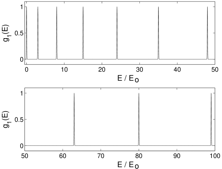
Figure 1: Numerical evaluation of the trace formula (12) for the infinite square well where $F_{1}(E)=(1+E/E_{0})^{1/2}-1$. In the figure, $E$ is plotted in units of $E_{0}$. To ensure uniform lineshapes, correct degeneracies, and strict numerical convergence, we have used the usual prescription used in numerical semiclassics (see, for example, Section 5.5 of Ref. brack ) which is to convolve the trace formula with a Gaussian of width $\sigma$. For this particular calculation, we have truncated the sum at $k_{\text{max}}=10^{4}$ while prescribing $\sigma=0.05$.

It may now be instructive to illustrate our results with a few examples:
1) Infinite Square-well. In this example, $W(x)=-\hbar\pi/(\sqrt{2m}L){\rm cot}(\pi x/L)$. It belongs to class I with $A=\hbar^{2}\pi^{2}/(2mL^{2})=E_{0}$, $B=1$, and $C=0$. The quantum spectrum of $V_{1}$ is given by $f(n)=n(n+2)E_{0}$, with $n=0,1,2,\ldots$ . Then $F_{1}(E)=(1+E/E_{0})^{1/2}-1$. A careful numerical evaluation of the trace formula (12) with this $F_{1}(E)$ reproduces the quantum spectrum (see Fig. 1). It is also easy to check Eq. (31) by evaluating the action integral of $W^{2}(x)$ analytically, and Eq. (22) using Eq. (30) ($\eta=1$).

2) 3-dimensional harmonic oscillator in the $l^{th}$ partial wave. In this example $W(r)=\sqrt{2m}\omega r/2-\hbar/(\sqrt{2m})(l+1)/r$. It belongs to class II with $A=\hbar\omega$, $B=1/(2l+2)$ and $C=-\sqrt{B}$. The quantum spectrum, measured from the lowest state in a fixed partial wave is $f(n)=2n\hbar\omega$, so $F(E)=E/(2\hbar\omega)$. Again, Eq. (31) may be checked explicitly.

To verify Eq. (22), we find from Eq. (36) that

$$\eta = {1\over 2}+{1\over 2}[\ell+{1\over 2}-\sqrt{\ell(\ell+1)}]$$ (37)

in this example. The first $1/2$ represents the usual half-integer quantisation in LOWKB, while the terms in square brackets arise from the sum of order $\hbar^{2}$ and higher corrections. As discussed in detail by Seetharaman SV84 and Barclay barclay they can be removed by adopting the Langer prescription. We have also checked other examples analytically.

In conclusion, we have given a new proof that lowest order SWKB quantisation is exact, starting from periodic orbit theory, rather than by examining the higher order WKB terms. The key ingredients have been an invertible algebraic expression for the energy spectrum, and Barclay and Maxwell’s barclay ; barcmax insight about shape invariant potentials.

R.K.B and D.W.L.S are grateful to NSERC for continuing research support under discovery grants.

References

• (1) F. Cooper, A. Khare, and U. Sukhatme, Supersymmetry in Quantum Mechanics, (World Scientific, Singapore, 2001), p. 36.
• (2) A. B. Migdal and V.P. Krainov, Approximate Methods in Quantum Mechanics (W. A. Benjamin Inc., N.Y., 1969) p. 119.
• (3) R. E. Langer, Phys. Rev. 51, 669 (1937).
• (4) D. T. Barclay, Phys. Lett. A 185, 169 (1994).
• (5) L. Gendenshtein, JETP Lett. 38, 356 (1983).
• (6) A. Comtet, A.D. Bandrauk and D.K. Campbell, Phys. Lett. B 150, 159 (1985).
• (7) R. Dutt, A. Khare and U. Sukhatme, Phys. Lett. B 181, 295 (1986); R. Adhikari, R. Dutt, A. Khare and U. Sukhatme, Phys. Rev. A 38, 1679 (1988).
• (8) M. Brack and R. K. Bhaduri, Semiclassical Physics (Westview Press, Boulder, Colorado, 2003).
• (9) R. Dutt, A. Khare, and U. Sukhatme, Am. J. Phys. 56, 163 (1988).
• (10) R. Balian and C. Bloch, Ann. Phys. (N. Y.) 60, 401 (1970); 63, 592 (1971); 69, 76 (1972).
• (11) B. K. Jennings, Ph.D. Thesis, McMaster University, 1976 (unpublished);
• (12) R. K. Bhaduri and C. K. Ross, Phys. Rev. Lett. 27, 606 (1971); B. K. Jennings, Ann. Phys. (N. Y.) 84, 1 (1974).
• (13) D. T. Barclay and C J. Maxwell, Phys. Lett. A 157, 357 (1991).
• (14) M. Seetharaman and S.S. Vasan, J. Phys. A 17, 2485 (1984).