Anharmonic effects on a phonon number measurement of a quantum mesoscopic mechanical oscillator

Abstract

We generalize a proposal for detecting single phonon transitions in a single nanoelectromechanical system (NEMS) to include the intrinsic anharmonicity of each mechanical oscillator. In this scheme two NEMS oscillators are coupled via a term quadratic in the amplitude of oscillation for each oscillator. One NEMS oscillator is driven and strongly damped and becomes a transducer for phonon number in the other measured oscillator. We derive the conditions for this measurement scheme to be quantum limited and find a condition on the size of the anharmonicity. We also derive the relation between the phase diffusion back-action noise due to number measurement and the localization time for the measured system to enter a phonon number eigenstate. We relate both these time scales to the strength of the measured signal, which is an induced current proportional to the position of the readout oscillator.

I Introduction

With device fabrication in the submicron or nanometer regime, it is possible to fabricate mechanical oscillators with very high fundamental frequencies and high mechanical quality factors. In the regime when the individual mechanical quanta are of the order of or greater than the thermal energy, quantum effects become important. Recently, a high-frequency mechanical resonator beam that operates at GHz frequencies has been reported HZMR03 . Unlike quantum optical systems where extremely high frequency oscillators, vacuum environments, zero temperature, and well-isolated systems are the usual setup, solid state systems normally exist at finite temperatures and interact with their surroundings. For a resonator operating at the fundamental frequency of GHz and at a temperature of 100mK, on average only 20 vibrational quanta are present in the fundamental mode. An interesting question is: can we observe quantum jumps, i.e., discrete (Fock or number state) transitions in such a true mechanical oscillator in a mesoscopic solid system R00 , as the mechanical oscillator exchanges quanta with the outside world or environment? In order to observe quantum jumps, one needs to design a scheme to measure the phonon number of the oscillator so that the oscillator will stay in a certain phonon number state long enough before it jumps to another phonon number state due to the inevitable interaction with its environment, usually through linear coupling to the oscillator position.

To achieve a quantum mechanical phonon number measurement of a mechanical oscillator, conventional measurement methods, such as the direct displacement measurement, BG03 cannot be simply applied since the observable (i.e., the number of phonons in the oscillator) does not commute with, for example, the position or displacement operator. Thus, naively attaching a readout transducer to the mechanical oscillator results in inaccurate subsequent measurements due to back action. One thus must make sure that the transducer that couples to the mechanical resonator measures only the mean-square position, without coupling linearly to the resonator’s position itself R00 .

Some preliminary experiments in this direction have been conducted . They use a second, driven mechanical oscillator (oscillator $1$ in Fig. 1) as the transducer to measure the mean-square position of the system oscillator (oscillator $0$ in Fig. 1). Hereafter, we use the notations of the “system oscillator” and “ancilla oscillator” in the text, but keep $0$ and $1$ as subscripts in the mathematical notations. The basic idea is that the non-linear, quadratic-in-position coupling between the two oscillators shifts the resonance frequency of the ancilla oscillator by an amount proportional to the phonon number or energy excitation of the system oscillator. This frequency shift may be detected as a phase shift of the oscillations of the ancilla oscillator with respect to the driving, when driven at a fixed frequency near resonance. Also, the ancilla oscillator needs to have sufficient sensitivity to resolve an individual quantum jump.

In the analysis of this measurement scheme presented by Santamore, Doherty, and Cross SDC03 , self-anharmonic terms $x_{i}^{4}$, in the two mechanical oscillators were neglected due to the smallness of the coupling coefficients compared to their harmonic oscillation frequencies, where $x_{i}$, $i=0,1$ is the displacement of the oscillators position from equilibrium. Since the self-anharmonic terms are of the same order as the nonlinear coupling term $x_{0}^{2}x_{1}^{2}$, it is important to include those terms and analyze the effects on the proposed measurement scheme.

In this paper, we extend the work of Ref. SDC03 and investigate the effects of self-anharmonic terms on a phonon number measurement. Due to the higher order self-anharmonic terms, the adiabatic elimination method used in Ref. SDC03 may not be straightforwardly applied even with the assumption of a heavily damped ancilla oscillator due to measurement. Here we take a slightly different approach. As the ancilla is assumed to be heavily damped, it will relax very rapidly to its steady state within a timescale on the order of typical response time of the system oscillator, and will appear to the system oscillator effectively as a “bath”. To see the consequences of a rapidly decaying ancilla oscillator on the dynamics of the system oscillator, we use the quantum open systems approach to find the master equation for the reduced density matrix of the system oscillator. In obtaining the master equation, the correlation functions of the “effective bath” (or the ancilla oscillator) are calculated using the generalized P-representation approach DG80 . The generalized P-representation approach has the advantage of removing some of the unnecessary restrictions imposed in Ref. SDC03 .

We find that in the presence of self-anharmonic term, $x_{1}^{4}$, of the ancilla oscillator, the effect of increasing driving strength and self-nonlinearity tends to shift the resonance frequency, increase the peak value and decrease the width of the response of the peak of $(\Gamma/\Gamma_{0})$ (see Fig. 2). The quantity $(\Gamma/\Gamma_{0})$ is the ratio of the back-action diffusion coefficient (or decoherence rate) $\Gamma$ [see Eq. (65)] and its value $\Gamma_{0}$ at zero self-anharmonicity and zero detuning. If the damping of the ancilla oscillator is much larger than the effect of the self-anharmonic term, the overall effect of self-anharmonic term on the phonon number measurement is small. Finally, we show that the induced electromotive readout current YGPB94 from the ancilla oscillator provides information on the phonon number of the system, even in the presence of higher order anharmonic terms, and we obtain the relation between the current and the measured system observable.

In the next section, we discuss briefly the measurement scheme and Hamiltonian, and obtain the master equation for the model described above while keeping higher order self-anharmonic terms. It turns out that the master equation we obtain requires two-time correlations of the ancilla oscillator operators. Section IV deals with this issue. We find one-time and two-time correlation functions of the ancilla. In Sec. V, we examine the effect of the self-anharmonic terms on the dynamics of the system oscillator from the master equation of its reduced density matrix. In Sec. VI, we obtain the dependence of the measurement current on the measured system oscillator observable, the phonon number.

II Hamiltonian and the master equation

II.1 Proposed scheme

Figure 1: Schematic of phonon number measurement for a coupled mechanical oscillator. Oscillators $0$ and $1$ are anharmonically coupled with coupling strength $\lambda_{01}$. Both oscillators are subjected to thermal noise injection and dissipation. The oscillator $1$ is driven and a readout apparatus is attached to it.

Our model consists of two mesoscopic scale mechanical bridges with rectangular cross section. One serves as a system oscillator (oscillator 0 in Fig. 1) to be measured. The other is used as an ancilla oscillator (oscillator 1 in Fig. 1), and is part of the measuring apparatus. Details of the scheme have been already discussed in Ref. SDC03 . A schematic illustration is reproduced in Fig. 1. These mesoscopic-size elastic bridges or beams with rectangular cross-section are connected by a device that transmits only one of the flexing modes of the system oscillator to the ancilla oscillator. As a result, these two resonators are anharmonically and symmetrically coupled (for experimental progress toward the scheme, see Ref. HZMR03 ). We label the measured system oscillator with subscript $0$ and the ancilla oscillator with subscript $1$, with corresponding resonant frequencies of the two flexing modes labelled as $\omega_{0}$ and $\omega_{1}$, respectively. The ancilla oscillator is driven at frequency $\omega_{d}$ with strength $\epsilon(t)$. A measuring apparatus is attached to the ancilla oscillator. The whole structure is subjected to the thermal bath environment. The interaction of the system oscillator with the thermal bath causes thermal dissipation and excitation of the system oscillator, which results in random-in-time transitions between phonon number eigenstates (i.e., quantum jumps). A change in the energy of the system oscillator appears to the ancilla oscillator as a shift of the resonant frequency via the anharmonic coupling. This frequency shift may be detected as a phase shift of the oscillations of the ancilla oscillator with respect to the driving, when driven at a fixed frequency near resonance.

II.2 Model Hamiltonian

The free Hamiltonian for the two bridge oscillators $0$ and $1$ is

$$H_{\mathrm{free}}=\hbar\omega_{0}a^{\dagger}a+\hbar\omega_{1}b^{\dagger}b,$$ (1)

where $a^{\dagger},a$ are creation and annihilation operators for oscillator $0$, respectively, and similarly, $b^{\dagger},b$ for oscillator $1$. The ancilla oscillator is driven at frequency $\omega_{d}$ with driving strength $\epsilon$,

$$H_{\mathrm{drive}}=\hbar\epsilon\cos\left[\omega_{d}t\right]\left(b^{\dagger}+b\right),$$ (2)

In the interaction picture, the driving term becomes

$$H_{\mathrm{drive}}^{\mathrm{I}}=2\hbar\epsilon\left(b^{\dagger}e^{+i\delta\omega}+be^{-i\delta\omega}\right),$$ (3)

where $\delta\omega$ is detuning between the ancilla resonant frequency and the driving frequency, $\omega_{1}-\omega_{d}$.

The two oscillators are coupled anharmonically through the special coupling device that controls and allows only one type of strain (the longitudinal stretch) to pass to other oscillator. Beyond the linear elasticity theory, the two flexing modes, which are perpendicular to each other, are coupled. Expansion of the elastic energy with respect to the strain tensor is taken up to second order. The next term, cubic in the elastic energy, gives quadratic terms in the equation of motion LL ; T . Since the coupling of the two modes of the two beams is symmetric, and since the two modes are not coupled at the linear level, the first order in coupling is $x_{0}^{2}x_{1}^{2}$, where $x_{i}$ is the displacement operator. So we expand the anharmonic terms up to first order in coupling and obtain

$$H_{anh} =\hbar\left(\tilde{\lambda}_{0}x_{0}^{2}+\tilde{\lambda}_{00}x_{0}^{4}+\tilde{\lambda}_{1}x_{1}^{2}+\tilde{\lambda}_{11}x_{1}^{4}\right),$$ (4)

$$V_{anh} =\hbar\tilde{\lambda}_{01}x_{0}^{2}x_{1}^{2},$$ (5)

where $\tilde{\lambda}_{ij}$ is the coupling coefficient. The high frequencies of the resonators, i.e., $(\omega_{0}-\omega_{1})$ much larger than $\tilde{\lambda}_{01}$ and their damping rates, allows us to use the rotating wave approximation. Thus we write the anharmonic terms as

$$H_{anh} =\hbar\lambda_{00}\left(a^{\dagger}a\right)^{2}+\hbar\lambda_{11}\left(b^{\dagger}b\right)^{2},$$ (6)

$$V_{anh} =\hbar\lambda_{01}a^{\dagger}ab^{\dagger}b,$$ (7)

where we have defined the standard raising and lowering operators for the oscillators: $a=\sqrt{m_{0}\omega_{0}/2\hbar}\;x_{0}+i\sqrt{1/2\hbar m_{0}\omega_{0}}\;p_{0}$, $a^{\dagger}$ is the Hermitian conjugate of $a$ and similarly for $b$ and $b^{\dagger}$ with the subscript $0$ replaced by $1$. We have also introduced new coefficients $\lambda$’s (without tildes) which all have the same dimension of frequency.

The coupling term $\lambda_{01}a^{\dagger}ab^{\dagger}b$ commutes with the observable $a^{\dagger}a$, enabling a quantum non-demolition (QND) measurement. The terms $\lambda_{0}a^{\dagger}a$ and $\lambda_{1}b^{\dagger}b$ shift the resonance frequency by a constant amount, so we have absorbed these quantities into $\omega_{0}$ and $\omega_{1}$. The terms $\hbar\lambda_{00}(a^{\dagger}a)^{2}$ and $\hbar\lambda_{11}(b^{\dagger}b)^{2}$ are analogous to Kerr non-linearities in nonlinear optics. Since these terms commute with the measured observable $(a^{\dagger}a)$, they will not change the system phonon number eigenstates; however, the Kerr effect causes an intensity dependent phase shift. Unlike a coherent state, in which this effect results in rotational shearing, a thermal state will not be affected by phase shift, due to its rotational invariance.

As for detecting phonon number in the system oscillator, we adapt a magnetomotive detection scheme suggested by Yurke et al YGPB94 ; CR96 ; CR99 . The voltage developed is proportional to $dx_{1}/dt$, where $x_{1}$ is the displacement of the beam from its equilibrium position. The current induced by this voltage is monitored by phase lock-in amplifier. An experimenter monitors the amplitude of the current and its phase with respect to the driving current that is set to a frequency near resonance. The details of the relation between the measured current and the phonon number of the system oscillator are derived in Ref. (SDC03 ).

There are two physically distinct environments in the model: the thermo-mechanical environment of each oscillator and the electronic noise environment of the electrical system that ultimately provides information on the motion of the ancilla. The environments are modelled as thermal baths, each consisting of an infinite number of harmonic oscillators. The couplings between the oscillators and the thermal baths are considered as weak, linear and Markovian; thus we use the rotating wave approximation. The Hamiltonian of the baths and their coupling to the oscillators can then be written as:

$$H_{bath} = \hbar\sum_{\mathrm{s}}\sum_{n}\omega_{\mathrm{s},i}B_{\mathrm{s},n}^{\dagger}B_{\mathrm{s},n},$$ (8)

$$V_{bath} = \hbar\left(\Omega_{B0}^{\dagger}\,a+a^{\dagger}\Omega_{B0}\right)+\hbar\left(\Omega_{B1}^{\dagger}\,b+b^{\dagger}\Omega_{B1}\right)+\hbar\left(\Omega_{Bm}^{\dagger}\,b+b^{\dagger}\Omega_{Bm}\right),$$ (9)

where $s$ runs over three different baths: the thermal baths coupled to the system oscillator ($B0$) and ancilla oscillator ($B1$), and the electronic (measurement) bath coupled to ancilla oscillator ($Bm$). The operator

$$\Omega_{\mathrm{s}}=\sum_{\mathrm{n}}g_{\mathrm{s}}\left(\omega_{n}\right)B_{s,n}$$ (10)

consists of bath operators, and the coupling to the bath modes is given by the coefficients $g_{\mathrm{s}}\left(\omega_{n}\right)$.

II.3 Master equation

Using the standard technique for open quantum systems, we first obtain the master equation for the joint density matrix of the two oscillators, $R$, by tracing out the bath variables:

$$\frac{dR}{dt} =-i\omega_{0}\left[a^{\dagger}a,R\right]-i\lambda_{00}\left[\left(a^{\dagger}a\right)^{2},R\right]$$

$$-i\delta\omega\left[b^{\dagger}b,R\right]-i\epsilon\left[b^{\dagger}+b,R\right]-i\lambda_{11}\left[\left(b^{\dagger}b\right)^{2},R\right]-i\lambda_{01}\left[a^{\dagger}ab^{\dagger}b,R\right]$$

$$+\nu\left(N_{0}+1\right)\mathcal{D}\left[a\right]R+\nu N_{0}\mathcal{D}\left[a^{\dagger}\right]R+\kappa\left(N_{1}+1\right)\mathcal{D}\left[b\right]R+\kappa N_{1}\mathcal{D}\left[b^{\dagger}\right]R,$$ (11)

where

$$\mathcal{D}\left[O\right]R =2ORO^{\dagger}-(O^{\dagger}OR+RO^{\dagger}O),$$ (12)

$$\mathcal{D}\left[O^{\dagger}\right]R =2O^{\dagger}RO-(OO^{\dagger}R+ROO^{\dagger}).$$ (13)

are defined for arbitrary operators $O$ and $R$. The damping rate of the system oscillator $\nu$ is given by

$$\nu\equiv\pi\varrho_{\mathrm{B0}}\left(\omega_{0}\right)\left|g_{\mathrm{B0}}\left(\omega_{0}\right)\right|^{2}.$$ (14)

It is related to the quality factor $Q_{0}$ of the system oscillator by $\nu=\omega_{0}/2Q_{0}$. We have combined the damping rates $\mu$ and $\eta$, due respectively to thermal bath and measurement on ancilla oscillator, into $\kappa=\mu+\eta$, where

$$\mu \equiv\pi\varrho_{\mathrm{Bm}}\left(\omega_{1}\right)\left|g_{\mathrm{Bm}}\left(\omega_{1}\right)\right|^{2},$$ (15)

$$\eta \equiv\pi\varrho_{\mathrm{B1}}\left(\omega_{1}\right)\left|g_{\mathrm{B1}}\left(\omega_{1}\right)\right|^{2}.$$ (16)

Here $\varrho_{\mathrm{s}}\left(\omega\right)$ is the density of states of bath $s$ at frequency $\omega$. The $N_{\mathrm{i}}$ are the Bose-Einstein factors:

$$N_{0}=\frac{1}{e^{\hbar\beta_{0}\omega_{0}}-1},$$ (17)

and $N_{1}=\left(\eta N_{\bar{1}}+\mu N_{\mathrm{m}}\right)/\kappa$, where

$$N_{\bar{1}}=\frac{1}{e^{\hbar\beta_{1}\omega_{1}}-1},\ N_{\mathrm{m}}=\frac{1}{e^{\hbar\beta_{\mathrm{m}}\omega_{1}}-1},$$ (18)

with $\beta_{\mathrm{i}}=\left(k_{\mathrm{B}}T_{s}\right)^{-1}$ and $T_{s}$ the temperature of bath $s$. In Eq. (11), the first and the second lines are the free Hamiltonian and non-linear Kerr effect terms for system and ancilla oscillators, respectively. The third line in Eq. (11) is associated with the anharmonic coupling, and the last two lines are consequences of the interactions with thermal baths.

III Effect of heavily damped ancilla oscillator

To proceed further towards a master equation for the reduced density matrix for the system oscillator alone, the ancilla oscillator is assumed to be heavily damped due to measurements, i.e., $\kappa\gg\lambda_{ij},\nu$. In this case, the ancilla oscillator will relax very rapidly to its steady state and appear to the system oscillator as a “bath”. In fact, if $\lambda_{11}\ll\omega_{1}$ and $\lambda_{01}\ll\kappa$, the ancilla oscillator in Eq. (11) will remain near a thermal steady state with average number $N_{1}$. However, we will relax the condition $\lambda_{11}\ll\omega_{1}$ and treat the interaction $\lambda_{01}$ term pertubatively.

To see the consequences of the rapid decay of the ancilla oscillator on the dynamics of the system oscillator, we use perturbation theory and expand the interaction Hamiltonian $H_{I}\left(t\right)=\lambda_{01}a^{\dagger}ab^{\dagger}b$ up to second order, and trace out the ancilla oscillator variables. This implies that we need to calculate the relevant steady state averages and correlation functions for the ancilla oscillator in the presence of the anharmonic term $\lambda_{11}\left(b^{\dagger}b\right)^{2}$.

In this case, the master equation for the reduced density matrix $\rho(t)$ for the system oscillator alone can be written as

$$\frac{d\rho(t)}{dt} =-i\omega_{0}\left[a^{\dagger}a,\rho(t)\right]-i\lambda_{00}\left[\left(a^{\dagger}a\right)^{2},\rho(t)\right]+\nu\left(N_{0}+1\right)\mathcal{D}\left[a\right]\rho(t)+\nu N_{0}\mathcal{D}\left[a^{\dagger}\right]\rho(t)$$

$$-i\text{Tr}_{1}\left[H_{I}\left(t\right),R_{\mathrm{eff}}(t)\right]-\int_{0}^{t}\text{Tr}_{1}\left[H_{I}\left(t\right),\left[H_{I}\left(t^{\prime}\right),R_{\mathrm{eff}}(t)\right]\right]dt^{\prime},$$ (19)

where $R_{\mathrm{eff}}(t)\approx\rho(t)\rho_{1}(t)$ is the effective joint density matrix of the two oscillators under the approximation that the ancilla oscillator is heavily damped, and $\rho_{1}(\infty)$ is the steady state density matrix operator for the ancilla oscillator. Explicitly, the second term of the last line of Eq. (19) can be written as

$$\int_{0}^{t}\text{Tr}_{1}\left[H_{I}\left(t\right),\left[H_{I}\left(t^{\prime}\right),R_{\mathrm{eff}}(t)\right]\right]dt^{\prime}$$

$$=-\left(\lambda_{01}\right)^{2}\int_{0}^{t}a^{\dagger}a\left(t\right)a^{\dagger}a\left(t^{\prime}\right)\rho(t)\left\langle b^{\dagger}b\left(t\right)b^{\dagger}b\left(t^{\prime}\right)\right\rangle dt^{\prime}+\left(\lambda_{01}\right)^{2}\int_{0}^{t}a^{\dagger}a\left(t\right)\rho(t)a^{\dagger}a\left(t^{\prime}\right)\left\langle b^{\dagger}b\left(t^{\prime}\right)b^{\dagger}b\left(t\right)\right\rangle dt^{\prime}$$

$$+\left(\lambda_{01}\right)^{2}\int_{0}^{t}a^{\dagger}a\left(t^{\prime}\right)\rho(t)a^{\dagger}a\left(t\right)\left\langle b^{\dagger}b\left(t\right)b^{\dagger}b\left(t^{\prime}\right)\right\rangle dt^{\prime}-\left(\lambda_{01}\right)^{2}\int_{0}^{t}\rho(t)a^{\dagger}a\left(t^{\prime}\right)a^{\dagger}a\left(t\right)\left\langle b^{\dagger}b\left(t^{\prime}\right)b^{\dagger}b\left(t\right)\right\rangle dt^{\prime}.$$ (20)

The exact correlation functions of the ancilla oscillator are not easy to evaluate because of the presence of the anharmonicity, the driving, and the decay terms. However, one can make an expansion of the state of the ancilla oscillator around its steady state and linearize the fluctuations, assuming them to be small WM ; DW80 .

Define the steady-state mean field amplitudes as $\left\langle b\right\rangle_{\infty}=\beta_{0}$. The operator $b$ can be written in terms of small fluctuations about the steady state mean value as

$$b\left(t\right)=\beta_{0}+b_{1}\left(t\right).$$ (21)

Then, keeping terms up to quadratic order in $b_{1},b_{1}^{\dagger},$ the interaction Hamiltonian $H_{I}=\lambda_{01}a^{\dagger}ab^{\dagger}b$ becomes

$$H_{I}=\lambda_{01}a^{\dagger}a\left[\left|\beta_{0}\right|^{2}+\beta_{0}^{\ast}b_{1}\left(t\right)+\beta_{0}b_{1}^{\dagger}\left(t\right)+b_{1}^{\dagger}\left(t\right)b_{1}\left(t\right)\right].$$ (22)

The first term in Eq. (22) contributes to a shift in the resonant frequency of the system oscillator by a constant amount and can be combined with the free Hamiltonian. Inserting this expression back into the first term of the last line of Eq. (19) gives the first order expansion term

$$-i\lambda_{01}\text{Tr}_{1}\left[a^{\dagger}a\left(t\right)b^{\dagger}b\left(t\right),R_{\mathrm{eff}}(t)\right]=-i\lambda_{01}\left[a^{\dagger}a\left(t\right),\rho\right]\left\langle b_{1}^{\dagger}b_{1}(t)\right\rangle,$$ (23)

where we have used the fact that averages of fluctuation fields vanish, i.e.,

$$\left\langle b_{1}\right\rangle=\left\langle b_{1}^{\dagger}\right\rangle=0.$$ (24)

Now we turn our attention to the second order term, Eq. (20). Note that since $\kappa\gg\nu$, the phonon number $a^{\dagger}a(t)$ of the system oscillator changes with time on a time scale much larger than $b^{\dagger}b(t)$ of the ancilla oscillator. So we can approximate $a^{\dagger}a(t^{\prime})\simeq a^{\dagger}a(t)$ in Eq. (20) and pull the system oscillator terms outside of the integral. Then Eq. (20) becomes

$$\int_{0}^{t}\text{Tr}_{1}\left[H_{I}\left(t\right),\left[H_{I}\left(t^{\prime}\right),R_{\mathrm{eff}}(t)\right]\right]dt^{\prime}$$

$$\approx\left(\lambda_{01}\right)^{2}\left\{a^{\dagger}a\left(t\right)\rho(t)a^{\dagger}a\left(t\right)-\left(a^{\dagger}a\left(t\right)\right)^{2}\rho(t)\right\}\int_{0}^{t}\left\langle B\left(t,t^{\prime}\right)\right\rangle dt^{\prime}$$

$$+\left(\lambda_{01}\right)^{2}\left\{a^{\dagger}a\left(t\right)\rho(t)a^{\dagger}a\left(t\right)-\rho(t)\left(a^{\dagger}a\left(t\right)\right)^{2}\right\}\int_{0}^{t}\left\langle B\left(t^{\prime},t\right)\right\rangle dt^{\prime}$$ (25)

where

$$\left\langle B\left(t,t^{\prime}\right)\right\rangle =\left(\beta_{0}^{\ast}\right)^{2}\left\langle b_{1}\left(t\right)b_{1}\left(t^{\prime}\right)\right\rangle+\left|\beta_{0}\right|^{2}\left\langle b_{1}\left(t\right)b_{1}^{\dagger}\left(t^{\prime}\right)\right\rangle+\left|\beta_{0}\right|^{2}\left\langle b_{1}^{\dagger}\left(t\right)b_{1}\left(t^{\prime}\right)\right\rangle+\left(\beta_{0}\right)^{2}\left\langle b_{1}^{\dagger}\left(t\right)b_{1}^{\dagger}\left(t^{\prime}\right)\right\rangle$$ (26)

$$\left\langle B\left(t^{\prime},t\right)\right\rangle =\left(\beta_{0}^{\ast}\right)^{2}\left\langle b_{1}\left(t^{\prime}\right)b_{1}\left(t\right)\right\rangle+\left|\beta_{0}\right|^{2}\left\langle b_{1}\left(t^{\prime}\right)b_{1}^{\dagger}\left(t\right)\right\rangle+\left|\beta_{0}\right|^{2}\left\langle b_{1}^{\dagger}\left(t^{\prime}\right)b_{1}\left(t\right)\right\rangle+\left(\beta_{0}\right)^{2}\left\langle b_{1}^{\dagger}\left(t^{\prime}\right)b_{1}^{\dagger}\left(t\right)\right\rangle$$ (27)

and higher order fluctuation terms than $b_{1}^{2}$ are ignored. The linearization transforms the second-order correlation functions of the ancilla operators, $\langle b^{\dagger}b(t)b^{\dagger}b(t^{\prime})\rangle$ and $\left\langle b^{\dagger}b\left(t^{\prime}\right)b^{\dagger}b\left(t\right)\right\rangle$, into first order correlation functions of fluctuation fields: $\langle b_{1}^{\dagger}\left(t\right)b_{1}\left(t^{\prime}\right)\rangle$, $\langle b_{1}^{\dagger}\left(t\right)b_{1}^{\dagger}\left(t^{\prime}\right)\rangle$ $\langle b_{1}^{\dagger}\left(t\right)b_{1}\left(t^{\prime}\right)\rangle$, and $\langle b_{1}^{\dagger}\left(t\right)b_{1}^{\dagger}\left(t^{\prime}\right)\rangle$.

IV One-time and two-time correlation functions of ancilla

In this section we calculate the one-time and two-time correlation functions of the ancilla oscillator. For this purpose, first we need to calculate the one-time correlation functions of a single driven anharmonic oscillator. We will follow the method of Drummond and Walls DW80 , who obtained one-time correlation functions. Then we extend their method to calculate two-time correlation functions.

The master equation for the driven, anharmonic ancilla oscillator interacting with the thermal bath is given by

$$\frac{d{\rho_{1}(t)}}{dt} =-i\delta\omega\left[b^{\dagger}b,\rho_{1}(t)\right]-i\epsilon\left[b^{\dagger}+b,\rho_{1}(t)\right]-i\lambda_{11}\left[\left(b^{\dagger}b\right)^{2},\rho_{1}(t)\right]$$

$$+\kappa\left(N_{1}+1\right)\mathcal{D}\left[b\right]\rho_{1}(t)+\kappa N_{1}\mathcal{D}\left[b^{\dagger}\right]\rho_{1}(t).$$ (28)

where $\rho_{1}$ is the density matrix of the ancilla oscillator and $\delta\omega=\omega_{1}-\omega_{d}$ is the detuning, with $\omega_{d}$ the driving frequency. The exact steady-state one-time correlation functions for a system with master equation Eq. (28) at zero temperature were given in Refs. WM ; DW80 , in a discussion of optical bistability of a coherently driven dispersive cavity with a cubic nonlinearity in the polarizability of the internal medium. At finite temperature, no exact solution has been found.

Our first objective is to derive a stochastic differential equation from the quantum master equation. Representing a density matrix in a coherent state basis is useful in systems described by Bose operators $b^{\dagger},b$. Due to the presence of the non-linear, self-anharmonic term, we will use the generalized P-representation introduced by Drummond and Gardiner DG80 to preserve the positivity of the Hermitian density operator.

Using the above transformations, the Fokker-Planck equation corresponding to the master equation Eq. (28) can now be written as

$$\frac{\partial}{\partial t}P\left(\hat{\beta}\right) =\left\{\frac{\partial}{\partial\beta}\left[\left(\kappa+i\delta\omega+i\lambda_{11}\right)\beta-2i\lambda_{11}\beta^{2}\alpha+i\epsilon\right]-i\lambda_{11}\frac{\partial^{2}}{\partial\beta^{2}}\beta^{2}\right.$$

$$\left.+\frac{\partial}{\partial\alpha}\left[\left(\kappa-i\delta\omega-i\lambda_{11}\right)\alpha-2i\lambda_{11}\alpha^{2}\beta-i\epsilon\right]-i\lambda_{11}\frac{\partial^{2}}{\partial\alpha^{2}}\alpha^{2}+2\kappa N_{1}\frac{\partial^{2}}{\partial\beta\partial\alpha}\right\}P\left(\hat{\beta}\right).$$ (29)

The argument of the generalized $P$ function is $\hat{\beta}=\left(\beta,\alpha\right)^{T}$. The correspondence principle between operators and $c$-numbers is as follows: $\beta\leftrightarrow b$ and $\alpha\leftrightarrow b^{\dagger}$. However, $\left(\beta,\alpha\right)$ are not complex conjugates. Drummond and Gardiner have shown DG80 that the Fokker-Planck equation in $\hat{\beta}$ can be transformed to a stochastic differential equation with positive definite diffusion . They found that the stochastic differential equations in the Ito calculus corresponding to Eq. (29) are

$$\frac{\partial}{\partial t}\left[\begin{array}[]{c}\beta\\ \alpha\end{array}\right]=\left[\begin{array}[]{c}-i\epsilon-\beta\left(\kappa+i\delta\omega+i\lambda_{11}+2i\lambda_{11}\beta\alpha\right)\\ i\epsilon-\alpha\left(\kappa-i\delta\omega-i\lambda_{11}-2i\lambda_{11}\alpha\beta\right)\end{array}\right]+\left[\begin{array}[]{cc}-2i\lambda_{11}\beta^{2}&2\kappa N_{1}\\ 2\kappa N_{1}&2i\lambda_{11}\alpha^{2}\end{array}\right]^{1/2}\left[\begin{array}[]{c}\xi_{1}\\ \xi_{2}\end{array}\right],$$ (30)

where $\xi_{1}$ and $\xi_{2}$ are random Gaussian functions, so that $\beta$ and $\alpha$ are complex conjugate in the mean . This stochastic differential equation is non-linear and not solvable as it is. However, it is reasonable to use a small noise expansion and linearize the fluctuations about the steady state of the mean field amplitudes. Thus we write $\beta$ in terms of the mean amplitude and first order expansion of the fluctuation,

$$\beta\left(t\right)=\beta_{0}+\beta_{1}\left(t\right),$$ (31)

where $\beta_{0}$ is the steady-state mean amplitude of $\beta$ and is given by

$$\beta_{0}=\frac{-i\epsilon}{i(\delta\omega+\lambda_{11}+2\lambda_{11}|\beta_{0}|^{2})+\kappa},$$ (32)

and $\beta_{1}$ is the zero mean fluctuation amplitude. We have a similar expression for $\alpha$. Thus $\beta_{0}$ and $\alpha_{0}$ are complex conjugate to each other (i.e., $\beta_{0}\alpha_{0}=\left|\alpha_{0}\right|^{2}=\left|\beta_{0}\right|^{2}\equiv n_{0}$). Then to first order in the fluctuations, the fluctuation amplitude vector $\hat{\beta}_{1}=(\beta_{1},\alpha_{1})^{T}$ obeys a stochastic differential equation

$$\frac{\partial}{\partial t}\hat{\beta}_{1}\left(t\right)=-\mathbf{A}\cdot\hat{\beta}_{1}\left(t\right)+\mathbf{D}^{1/2}\left(\hat{\beta}_{0}\right)\hat{\xi}\left(t\right),$$ (33)

where $\hat{\xi}=(\xi_{1},\xi_{2})^{T}$ is the noise vector, $\mathbf{A}$ is the linearized drift matrix and $\mathbf{D}$ is the diffusion matrix evaluated at $\hat{\beta}=\hat{\beta}_{0}.$ The matrices $\mathbf{A}$ and $\mathbf{D}$ are

$$\mathbf{A}=\left[\begin{array}[]{cc}\kappa+i\delta\omega+i\lambda_{11}+4i\lambda_{11}n_{0}&2i\lambda_{11}\beta_{0}^{2}\\ -2i\lambda_{11}\alpha_{0}^{2}&\kappa-i\delta\omega-i\lambda_{11}-4i\lambda_{11}n_{0}\end{array}\right],$$ (34)

and

$$\mathbf{D}=\left[\begin{array}[]{cc}-2i\lambda_{11}\beta_{0}^{2}&2\kappa N_{1}\\ 2\kappa N_{1}&2i\lambda_{11}\alpha_{0}^{2}\end{array}\right].$$ (35)

The one-time correlation matrix can be calculated using the method of Chaturvedi, et al CGMW77 ; WM ; DW80 ; G85 :

$$\mathbf{C}\left(t,t\right) =\left[\begin{array}[]{cc}\left\langle\beta_{1}^{2}\right\rangle&\left\langle\beta_{1}\alpha_{1}\right\rangle\\ \left\langle\alpha_{1}\beta_{1}\right\rangle&\left\langle\alpha_{1}^{2}\right\rangle\end{array}\right]$$ (38)

$$=\frac{1}{\Lambda^{2}}\left[\begin{array}[]{cc}-i\lambda_{11}\beta_{0}^{2}\left(\kappa-i\delta\omega-i\lambda_{11}-4i\lambda_{11}n_{0}\right)\left(2N_{1}+1\right)&N_{1}\left|\kappa+i\delta\omega+i\lambda_{11}+4i\lambda_{11}n_{0}\right|^{2}+2\lambda_{11}^{2}n_{0}^{2}\\ N_{1}\left|\kappa+i\delta\omega+i\lambda_{11}+4i\lambda_{11}n_{0}\right|^{2}+2\lambda_{11}^{2}n_{0}^{2}&i\lambda_{11}\alpha_{0}^{2}\left(\kappa+i\delta\omega+i\lambda_{11}+4i\lambda_{11}n_{0}\right)\left(2N_{1}+1\right)\end{array}\right],$$ (41)

where

$$\Lambda^{2} = \kappa^{2}+\Lambda_{1}^{2},$$ (42)

$$\Lambda_{1}^{2} = \left(\delta\omega+\lambda_{11}\right)^{2}+8\left(\delta\omega+\lambda_{11}\right)\lambda_{11}n_{0}+12\lambda_{11}^{2}n_{0}^{2}.$$ (43)

We now derive an expression for the two-time steady state correlation matrix

$$\mathbf{C}\left(t,t^{\prime}\right)=\left[\begin{array}[]{cc}\left\langle\beta_{1}\left(t\right)\beta_{1}\left(t^{\prime}\right)\right\rangle&\left\langle\beta_{1}\left(t\right)\alpha_{1}\left(t^{\prime}\right)\right\rangle\\ \left\langle\alpha_{1}\left(t\right)\beta_{1}\left(t^{\prime}\right)\right\rangle&\left\langle\alpha_{1}\left(t\right)\alpha_{1}\left(t^{\prime}\right)\right\rangle\end{array}\right]\;.$$ (44)

For $t>t^{\prime}$

$$\mathbf{C}\left(t,t^{\prime}\right)=\exp\left(-\mathbf{A}\left(t-t^{\prime}\right)\right)\mathbf{C}\left(t,t\right),$$ (45)

and for $t<t^{\prime}$

$$\mathbf{C}\left(t,t^{\prime}\right)=\mathbf{C}\left(t,t\right)\exp\left(-\mathbf{A}^{T}\left(t^{\prime}-t\right)\right).$$ (46)

Let us define $\mathbf{M}(t,t^{\prime})\equiv\exp[-\mathbf{A}(t-t^{\prime})]$. The matrix $\mathbf{M}$ can be calculated as follows. Let the matrix $\mathbf{U=}\left(u_{1},u_{2}\right)$ diagonalize $\mathbf{A}$ with eigenvalues $\lambda_{\pm}$. The eigenvalues for this $2\times 2$ matrix can be found from the characteristic equation:

$$\lambda_{\pm} =\frac{\mathrm{Tr}\left(\mathbf{A}\right)\pm\sqrt{\left[\mathrm{Tr}\left(\mathbf{A}\right)\right]^{2}-4\det\left(\mathbf{A}\right)}}{2}$$

$$=\kappa\pm i\Lambda_{1},$$ (47)

We then obtain the matrix $\mathbf{M}$ as

$$\mathbf{M}(t,t^{\prime}) = \boldsymbol{U}\left[\begin{array}[]{cc}\exp\left(-\lambda_{+}\left(t-t^{\prime}\right)\right)&0\\ 0&\exp\left(-\lambda_{-}\left(t-t^{\prime}\right)\right)\end{array}\right]\boldsymbol{U}^{-1}$$ (50)

$$= \frac{1}{2\Lambda_{1}}\left[\begin{array}[]{cc}\left(\Lambda_{1}-c\right)e^{-\lambda_{-}\left(t-t^{\prime}\right)}+\left(\Lambda_{1}+c\right)e^{-\lambda_{+}\left(t-t^{\prime}\right)}&2\lambda_{11}\beta_{0}^{2}\left[-e^{-\lambda_{-}\left(t-t^{\prime}\right)}+e^{-\lambda_{+}\left(t-t^{\prime}\right)}\right]\\ 2\lambda_{11}\alpha_{0}^{2}\left[e^{-\lambda_{-}\left(t-t^{\prime}\right)}-e^{-\lambda_{+}\left(t-t^{\prime}\right)}\right]&\left(\Lambda_{1}+c\right)e^{-\lambda_{-}\left(t-t^{\prime}\right)}+\left(\Lambda_{1}-c\right)e^{-\lambda_{+}\left(t-t^{\prime}\right)}\end{array}\right],$$ (53)

where $c\equiv 4\lambda_{11}n_{0}+\delta\omega+\lambda_{11}$. The two-time correlation matrix Eq. (44), then follows directly from Eqs. (45) (46) and (53), as well as the fact that $\exp[-\mathbf{A}(t-t^{\prime})]=\mathbf{M}(t,t^{\prime})$ and $\exp[-\mathbf{A}^{T}(t^{\prime}-t)]=\mathbf{M}^{T}(t^{\prime},t)$:

The detailed expressions of the two-time correlation functions are shown in the Appendix. We note that in the P-representation, the $c$-number time correlation function corresponds to a normally ordered time correlation function of the operators; thus the correlations above do not correspond to all the two-time correlation functions we need to find. For non-normally ordered time correlation functions, some care needs to be exercised. Using the procedure described, for example, in Refs. G85 ; GP00 , we obtain the following operator to $c$-number correspondence:

$$\left\langle b_{1}\left(t\right)b_{1}\left(t^{\prime}\right)\right\rangle =\left\langle\beta_{1}\left(t\right)\beta_{1}\left(t^{\prime}\right)\right\rangle,$$ (54)

$$\left\langle b_{1}\left(t\right)b_{1}^{\dagger}\left(t^{\prime}\right)\right\rangle =\left\langle\beta_{1}\left(t\right)\alpha_{1}\left(t^{\prime}\right)\right\rangle+M_{11}(t,t^{\prime}),$$ (55)

$$\left\langle b_{1}^{\dagger}\left(t\right)b_{1}\left(t^{\prime}\right)\right\rangle =\left\langle\alpha_{1}\left(t\right)\beta_{1}\left(t^{\prime}\right)\right\rangle,$$ (56)

$$\left\langle b_{1}^{\dagger}\left(t\right)b_{1}^{\dagger}\left(t^{\prime}\right)\right\rangle =\left\langle\alpha_{1}\left(t\right)\alpha_{1}\left(t^{\prime}\right)\right\rangle+M_{21}(t,t^{\prime}),$$ (57)

$$\left\langle b_{1}\left(t^{\prime}\right)b_{1}\left(t\right)\right\rangle =\left\langle\beta_{1}\left(t\right)\beta_{1}\left(t^{\prime}\right)\right\rangle+M_{12}(t,t^{\prime}),$$ (58)

$$\left\langle b_{1}\left(t^{\prime}\right)b_{1}^{\dagger}\left(t\right)\right\rangle =\left\langle\alpha_{1}\left(t\right)\beta_{1}\left(t^{\prime}\right)\right\rangle+M_{22}(t,t^{\prime}),$$ (59)

$$\left\langle b_{1}^{\dagger}\left(t^{\prime}\right)b_{1}\left(t\right)\right\rangle =\left\langle\beta_{1}\left(t\right)\alpha_{1}\left(t^{\prime}\right)\right\rangle,$$ (60)

$$\left\langle b_{1}^{\dagger}\left(t^{\prime}\right)b_{1}^{\dagger}\left(t\right)\right\rangle =\left\langle\alpha_{1}\left(t\right)\alpha_{1}\left(t^{\prime}\right)\right\rangle,$$ (61)

where $M_{ij}(t,t^{\prime})$ are the matrix elements of the matrix $\mathbf{M}(t,t^{\prime})$, Eq. (53).

V Master Equation for a reduced density matrix

Having found the one-time and two-time correlation functions, we can now evaluate Eqs. (23) and (25) and obtain the master equation for the reduced density matrix of the system oscillator as:

$$\frac{d\rho}{dt} =-i\left(\omega_{0}+\Delta\right)\left[a^{\dagger}a,\rho\right]-i\Theta\left[\left(a^{\dagger}a\right)^{2},\rho\right]-\Gamma\left[a^{\dagger}a,\left[a^{\dagger}a,\rho\right]\right]$$

$$+\nu\left(N_{0}+1\right)\mathcal{D}\left[a\right]\rho+\nu N_{0}\mathcal{D}\left[a^{\dagger}\right]\rho$$ (62)

where

$$\Delta ={\lambda_{01}}\left[n_{0}+\frac{1}{\Lambda^{2}}\left(N_{1}\left|\kappa+i\delta\omega+i\lambda_{11}+4i\lambda_{11}n_{0}\right|^{2}+2\lambda_{11}^{2}n_{0}^{2}\right)\right],$$ (63)

$$\Theta =\lambda_{00}+\frac{\lambda_{01}^{2}n_{0}}{\Lambda^{2}}\left(\delta\omega+i\lambda_{11}+2\lambda_{11}n_{0}\right),$$ (64)

$$\Gamma =\frac{\lambda_{01}^{2}}{\Lambda^{4}}\kappa n_{0}(2N_{1}+1)\left[\left|\kappa+i\delta\omega+i\lambda_{11}+4i\lambda_{11}n_{0}\right|^{2}-4\lambda_{11}n_{0}(\delta\omega+\lambda_{11}+3\lambda_{11}n_{0})\right]$$

$$=\frac{\lambda_{01}^{2}}{\Lambda^{4}}\kappa\epsilon^{2}(2N_{1}+1).$$ (65)

We have set $n_{0}=\left|\beta_{0}\right|^{2}$, and $\Lambda^{2}$ is defined in Eqs. (42) and (43). In obtaining the last line of Eq. (65), we have used Eq. (32).

In Eq. (62), $\Delta$ in the first term is the resonant frequency shift due to interactions. The second term is the Kerr non-linear phase shift, with coefficient $\Theta$ depending on the anharmonicity of both oscillators $\lambda_{00}$ and $\lambda_{11}$, as well as the detuning of the ancilla oscillator. The parameter $\Gamma$ is the phase diffusion coefficient or decoherence rate, associated with back-action due to an effective measurement of $a^{\dagger}a$. Physically, due to monitoring, the system would localize or collapse into a phonon number eigenstate on a time scale of order $\Gamma^{-1}$. The measurement time that is needed for the measurement apparatus to distinguish one state from the next is also proportional to $\Gamma^{-1}$. The last two terms in Eq. (62), can be derived from the thermal coupling to the system and are responsible for the quantum jumps. In the case when $\nu=0$, the conditional master equation of Eq. (62) will describe a QND measurement of the system oscillator phonon number. The time the system stays in a given phonon number state before making a transition due to either excitation or relaxation is proportional to $\nu^{-1}$. To be a good quantum measurement of a phonon number state, we want the system’s dwelling time to be long compared to the time necessary to determine which number state the system is in, i.e., $(\Gamma/\nu)\gg 1$.

V.1 Effects of the anharmonic terms

From Eq. (62), we notice several important points. Firstly, in the case of no detuning and no non-linear self-anharmonic terms (i.e., $\delta\omega=0,$ $\lambda_{00}=\lambda_{11}=0$), we have

$$\Delta =\lambda_{01}\left[N_{1}+(\epsilon/\kappa)^{2}\right],$$ (66)

$$\Theta =0,$$ (67)

$$\Gamma =\frac{\lambda_{01}^{2}\epsilon^{2}\left(2N_{1}+1\right)}{\kappa^{3}}.$$ (68)

These results agree with the results of a simpler model discussed in Ref. SDC03 , using a slightly different adiabatic elimination approach.

Secondly, the steady state solution Eq. (32) of Eq. (30) gives

$$\left|\epsilon\right|^{2}=n_{0}\left[\kappa^{2}+\left(\delta\omega+\lambda_{11}+2\lambda_{11}n_{0}\right)^{2}\right].$$ (69)

Equation (69) has an analogy to a classical anharmonic oscillatorLL1 . Bistability due to a Kerr nonlinearity is a well known phenomenon. Classically the oscillator will take one or the other of the stable solutions. Using Hurwitz stability criterion, to obtain stable solution for Eqs. (33)– (35) it is necessary to have

$$\mathrm{Tr}(\mathbf{A}{}) > 0,$$ (70)

$$\mathrm{Det}({}\mathbf{A}) > 0.$$ (71)

For the matrix , Eq. (34), gives $\mathrm{Tr}(\mathbf{A}{})=2\kappa>0$ for a dissipative or loss mechanism. Therefore the threshold points are determined by $\mathrm{Det}(\mathbf{A}{})=\Lambda^{2}=0$. However, in the quantum regime at zero temperature, bistability appears only during transient period and does not exist in the steady state.WM ; DG80 We, nevertheless, note that the linear theory that we use to calculate the steady state correlation functions at finite temperatures would break down at the instability points.

Secondly, from Eqs. (62) and (65), we see that when $\delta\omega=0$, the condition $\kappa\gg\lambda_{11}$ makes the effect of the non-linear self-anharmonic terms in $\Delta$ and $\Gamma$ very small, which justifies the assumption of neglecting $\lambda_{11}$ in Ref. SDC03 . However, our calculation allows us to do a quantitative analysis without making this assumption.

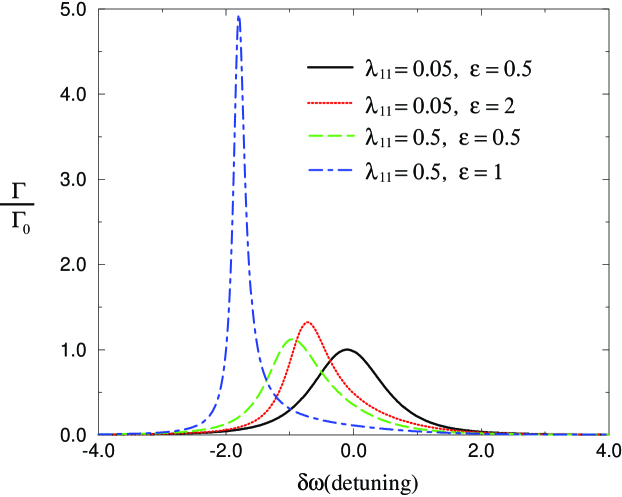
Figure 2: The ratio of $(\Gamma/\Gamma_{0})$ as a function of detuning at different values of driving strength and self-anharmonicity (Kerr effect coupling). The parameters are presented in unit of the damping rate $\kappa$.

The value of the phase diffusion coefficient $\Gamma$ (as compared to the damping rate $\nu$) is important to the phonon number measurement scheme and to the observation of quantum jumps. To see the effects of self-anharmonicity, driving and detuning on the phase diffusion coefficient $\Gamma$ compared to its value $\Gamma_{0}$ at zero self-anharmonic coupling and zero detuning ($\lambda_{11}=\epsilon=0$) SDC03 , we plot their ratio

$$\frac{\Gamma}{\Gamma_{0}}=\frac{\kappa^{4}}{\Lambda^{4}}$$ (72)

in Fig. 2. Note that $\Gamma$ diverges at $\Lambda^{2}=0$, which are the instability points where the linear theory is not valid. The parameters (in units of $\kappa$) in Fig. 2 are chosen so that the ancilla oscillator is away from these points. For example, if we were to increase further the driving strength in the dot-dashed line plot of Fig. 2, to $\epsilon=1.2$, say, the ancilla oscillator would then be in the instability regime. When the nonlinearity $\lambda_{11}$ is small, the solid line plot in Fig. 2 shows the linear resonance of small driving. The dotted, dashed, and dot-dashed line plots illustrate that increasing the driving strength and the nonlinearity tends to shift the resonance frequency, increase the peak value and decrease the width of the peak of $(\Gamma/\Gamma_{0})$.

Carr and Wybourne have estimated an anharmonic coefficient $\lambda_{ii}$ for a beam with rectangular cross-sectionCLW02 :

$$\lambda_{ii}=\frac{\pi^{4}}{128}\frac{\hbar B}{\rho_{i}^{2}\omega_{i}^{2}L_{i}^{5}w_{i}t_{i}},$$ (73)

where $B$ is the bulk modulus, $\rho_{i}$ is the mass density, $L,w,t$ are the dimensions of the beam: length, width, thickness, respectively. A simple estimation of $\kappa$ and $\lambda_{11}$ using realistic values for a mesoscopic mechanical oscillator reveals that $\lambda_{11}$ is many order of magnitude smaller than $\kappa$.

VI Measurement current

In the measurement scheme, we do not observe the phonon number of the system oscillator directly. Rather we perform a phase sensitive, ‘homodyne’, measurement on the quadrature $(b+b^{\dagger})$ of the ancilla oscillator. It is therefore important to show that an observation of the average current $\langle I\rangle=\sqrt{2\mu}\langle b+b^{\dagger}\rangle$ indeed corresponds to a phonon number measurement of the system oscillator. We anticipate that the average measured current of the ancilla oscillator is proportional to the average phonon number in the measured system oscillator. In addition we need to show that the coefficient of proportionality is related to the localization rate, which determines how long it takes to distinguish one number state from the next. Thus a strong signal corresponds to a rapid localization rate. Furthermore we expect that the localization rate is proportional to the backaction induced phase diffusion coefficient $\Gamma$, so that the better the measurement, the larger is the back action noise.

To demonstrate this, firstly we use the Hamiltonian to obtain the quantum Langevin equation for the ancilla oscillator operator $b$:

$$\frac{db}{dt} = -i\epsilon-i\delta\omega b-i\lambda_{01}a^{\dagger}ab-i2\lambda_{11}b^{\dagger}bb-\left[\eta b\left(t\right)-\sqrt{2\eta}B_{in}\left(t\right)\right]-\left[\mu b\left(t\right)-\sqrt{2\mu}D_{in}\left(t\right)\right],$$ (74)

$$\frac{db^{\dagger}}{dt} = i\epsilon+i\delta\omega b^{\dagger}+i\lambda_{01}a^{\dagger}ab^{\dagger}+i2\lambda_{11}b^{\dagger}b^{\dagger}b-\left[\eta b^{\dagger}\left(t\right)-\sqrt{2\eta}B_{in}^{\dagger}\left(t\right)\right]-\left[\mu b^{\dagger}\left(t\right)-\sqrt{2\mu}D_{in}^{\dagger}\left(t\right)\right],$$ (75)

where $B_{in}\left(t\right)$ is the input noise GP00 . The steady state [$(db/dt)=0$] average of $\langle b\rangle=\beta_{0}$ for the ancilla oscillator in isolation (i.e., with $\lambda_{01}=0$) is given by the same expression as Eq. (32). Linearizing around the steady state, renaming the operator describing the quantum fluctuation as $b_{1}(t)$, and assuming that $a^{\dagger}a$ do not to change appreciably over the typical time scale of the ancilla oscillator, we obtain

$$\frac{db_{1}}{dt} = -i(\delta\omega+\lambda_{11})b_{1}+2\lambda_{11}(2n_{0}b_{1}+\beta_{0}^{2}b_{1}^{\dagger})+\lambda_{01}\beta_{0}a^{\dagger}a-\kappa b_{1}+\sqrt{2\eta}B_{in}+\sqrt{2\mu}D_{in}$$ (76)

$$\frac{db_{1}^{\dagger}}{dt} = i(\delta\omega+\lambda_{11})b_{1}^{\dagger}+2\lambda_{11}(2n_{0}b_{1}^{\dagger}+(\alpha_{0}^{2}b_{1}^{\dagger})+\lambda_{01}\alpha_{0}a^{\dagger}a-\kappa b_{1}^{\dagger}+\sqrt{2\eta}B_{in}^{\dagger}+\sqrt{2\mu}D_{in}^{\dagger}.$$ (77)

or equivalently,

$$\frac{d}{dt}\left(\begin{array}[]{c}b_{1}\\ b_{1}^{\dagger}\end{array}\right)=\mathbf{A}\left(\begin{array}[]{c}b_{1}\\ b_{1}^{\dagger}\end{array}\right)+\left(\begin{array}[]{c}\lambda_{01}\beta_{0}a^{\dagger}a+\sqrt{2\eta}B_{in}+\sqrt{2\mu}D_{in}\\ \lambda_{01}\alpha_{0}a^{\dagger}a+\sqrt{2\eta}B_{in}^{\dagger}+\sqrt{2\mu}D_{in}^{\dagger}\end{array}\right),$$ (78)

where $\mathbf{A}$ is defined in Eq. (34). To calculate $\langle b+b^{\dagger}\rangle=\beta_{0}+\alpha_{0}+\langle b_{1}+b_{1}^{\dagger}\rangle$ in the steady state, we setting $(db_{1}/dt)=0=(db_{1}^{\dagger}/dt)$ in Eq. (78), to obtain

$$\left(\begin{array}[]{c}\langle b_{1}\rangle\\ \langle b_{1}^{\dagger}\rangle\end{array}\right)=\mathbf{A}^{-1}\left(\begin{array}[]{c}\lambda_{01}\beta_{0}a^{\dagger}a\\ \lambda_{01}\alpha_{0}a^{\dagger}a\end{array}\right).$$ (79)

Then after a simple calculation, we obtain the measured mean signal

$$\sqrt{2\mu}\,\langle b_{1}+b_{1}^{\dagger}\rangle = -i\sqrt{2\mu}\,\frac{\lambda_{01}}{\Lambda^{2}}\left\{\left[\left(\kappa-i(\delta\omega+\lambda_{11}+4\lambda_{11}|\beta_{0}|^{2})+2i\lambda_{11}(\alpha_{0})^{2}\right)\beta_{0}\right]-h.c.\right\}\langle a^{\dagger}a\rangle$$ (80)

$$= -i\sqrt{2\mu}\,\frac{\lambda_{01}}{\Lambda^{2}}\left[\kappa(\beta_{0}-\alpha_{0})-i(\delta\omega+\lambda_{11}+2\lambda_{11}|\beta_{0}|^{2})(\beta_{0}+\alpha_{0})\right]\langle a^{\dagger}a\rangle.$$

Using Eq. (32), we can simplify Eq. (80) further and obtain

$$\sqrt{2\mu}\,\langle b_{1}+b_{1}^{\dagger}\rangle=-\sqrt{2\mu}\,\frac{2\epsilon\,\lambda_{01}}{\Lambda^{2}}\langle a^{\dagger}a\rangle.$$ (81)

We note that the coefficient on the right hand side of Eq.(81) is proportional to $\sqrt{\Gamma}$, with a proportionality factor given by $-\sqrt{8\mu/\kappa(2N_{1}+1)}$. As the actual readout current is simply proportional to the average position of the ancilla oscillator R00 , Eq.(81) gives the expected proportionality between the average measured current and the average phonon number of the system oscillator.

In a typical experimental run, the measured current will contain a noise component made up of thermo-electrical noise in the transducer circuit as well as intrinsic quantum noise that arises directly from the back action noise when we measure phonon number. In order for the measurement to be quantum limited, we need to ensure that the dominant source of noise is back action noise. Recently, considerable progress towards this limit has been made in a nanoelectromechanical system Schwab04

VII Conclusions

We have investigated a scheme for the QND measurement of phonon number (cf SDC03 ) using two anharmonically coupled modes of oscillation of mesoscopic elastic bridges. We have included the self-anharmonic terms neglected in the previous analysis SDC03 , and analyzed the effect of higher order anharmonic terms in the approximation that the ancilla oscillator is heavily damped. We have shown that in the presence of self-anharmonic term, $x_{1}^{4}$, of the ancilla oscillator, the effect of increasing driving strength and self-nonlinearity tends to shift the resonance frequency, increase the peak value and decrease the width of the response of the peak of $(\Gamma/\Gamma_{0})$ as shown in Fig. 2. If the damping of the ancilla oscillator is much larger than the effect of the self-anharmonic term, the overall effect of self-anharmonic term on the phonon number measurement is small for small detuning, justifying the assumption of neglecting the self-anharmonic term at zero detuning in Ref. SDC03 . Our calculation, however, allows one to do a quantitative analysis at finite detuning and without making this assumption.

The key idea of the measurement scheme is that, from the point of view of the ancilla oscillator, the interaction with the system oscillator constitutes a shift in resonance frequency that is proportional to the time-averaged phonon number or energy excitation of the system oscillator. This frequency shift may be detected through a phase sensitive readout of the position of the driven readout oscillator. In a magnetic field, a wire patterned on the moving readout oscillator will result in an induced current which can be directly monitored by electrical means YGPB94 . The current gives direct access to the position of the ancilla oscillator and, through the mechanism described in this paper, to the phonon number of the measured system oscillator, even in the presence of the self-anharmonic terms. We have shown that this scheme realizes an ideal QND measurement of phonon number in the limit that the back action induced phase diffusion rate is much larger than the rate at which transitions occur between phonon number states, $(\Gamma/\nu)\rightarrow\infty$. When the ratio $(\Gamma/\nu)$ is finite and large, it is then possible to observe, in the readout current, quantum jumps between Fock (number states) in a mesoscopic mechanical oscillator, as the mechanical oscillator exchanges quanta with the environment.

We briefly discuss below some possible realistic values for $\Gamma$ and $\nu$. The value of $\Gamma_{0}$ depends on external driving, as well as materials and dimensions of the mechanical beams (oscillators). Here we quote the example in Ref. SDC03 using two GaAs mechanical oscillators with resonance frequencies $\omega_{0}=2.3$ GHz, $\omega_{1}=0.36$ GHz, and Q-factors $Q_{0}=10000$, $Q_{1}=1000$. The dimensions of the system oscillator are $0.6$ $\mu$m $\times$ $0.04$ $\mu$m $\times$ $0.07$ $\mu$m and those of the ancilla oscillator are $0.6$ $\mu$m $\times$ $0.04$ $\mu$m $\times$ $0.01$ $\mu$m. With the magnetic field $10$ Tesla and the driving current $1$ $\mu$A, $\Gamma_{0}$ and $\nu$ will be $\Gamma_{0}\approx 1.5\times 10^{4}$/s and $\nu\approx 1.2\times 10^{6}$/s, or $\Gamma_{0}/\nu=0.013$. A clear observation of quantum jumps requires $\Gamma_{0}/\nu\gg 1$, so that the present example is two orders of magnitude below the desired parameter regime. To increase the ratio of $\Gamma$ to $\nu$ we can improve on some of the parameters. One way is to increase the Q-factor of the system oscillator. Another way is to use lower density material such as carbon nanotubes as well as to decrease the thickness of the oscillator. These improvements are feasible with current fabrication technology. In addition, it is also possible to engineer the nonlinear coupling between the oscillators SP:Y . Furthermore, different driving and detection schemes other than magnetomotive detection can be considered to increase the driving strength. Given the steady improvement in the fabrication technology and experimental techniques, we believe that observing quantum jumps between phonon number states in a mesoscopic oscillator will be possible in the near future.

Appendix A Expressions for the two-time correlation functions

The two-time correlation functions in the main text for $C\left(t,t^{\prime}\right)$, where $t>t^{\prime}$, are

$$\left\langle\beta_{1}\left(t\right)\beta_{1}\left(t^{\prime}\right)\right\rangle =\frac{1}{2\Lambda_{1}}\left\{\left(\Lambda_{1}+c\right)\exp\left[-\lambda_{+}\left(t-t^{\prime}\right)\right]+\left(\Lambda_{1}-c\right)\exp\left[-\lambda_{-}\left(t-t^{\prime}\right)\right]\right\}\left\langle\beta_{1}^{2}\right\rangle$$

$$+\frac{\lambda_{11}\beta_{0}^{2}}{\Lambda_{1}}\left\{\exp\left[-\lambda_{+}\left(t-t^{\prime}\right)\right]-\exp\left[-\lambda_{-}\left(t-t^{\prime}\right)\right]\right\}\left\langle\beta_{1}\alpha_{1}\right\rangle,$$ (82)

$$\left\langle\alpha_{1}\left(t\right)\beta_{1}\left(t^{\prime}\right)\right\rangle =\frac{1}{2\Lambda_{1}}\left\{\left(\Lambda_{1}+c\right)\exp\left[-\lambda_{+}\left(t-t^{\prime}\right)\right]+\left(\Lambda_{1}-c\right)\exp\left[-\lambda_{-}\left(t-t^{\prime}\right)\right]\right\}\left\langle\alpha_{1}\beta_{1}\right\rangle$$

$$+\frac{\lambda_{11}\beta_{0}^{2}}{\Lambda_{1}}\left\{\exp\left[-\lambda_{+}\left(t-t^{\prime}\right)\right]-\exp\left[-\lambda_{-}\left(t-t^{\prime}\right)\right]\right\}\left\langle\alpha_{1}^{2}\right\rangle,$$ (83)

$$\left\langle\beta_{1}\left(t\right)\alpha_{1}\left(t^{\prime}\right)\right\rangle =\frac{-\lambda_{11}\alpha_{0}^{2}}{\Lambda_{1}}\left\{\exp\left[-\lambda_{+}\left(t-t^{\prime}\right)\right]-\exp\left[-\lambda_{-}\left(t-t^{\prime}\right)\right]\right\}\left\langle\beta_{1}^{2}\right\rangle$$

$$+\frac{1}{2\Lambda_{1}}\left\{\left(\Lambda_{1}-c\right)\exp\left[-\lambda_{+}\left(t-t^{\prime}\right)\right]+\left(\Lambda_{1}+c\right)\exp\left[-\lambda_{-}\left(t-t^{\prime}\right)\right]\right\}\left\langle\beta_{1}\alpha_{1}\right\rangle,$$ (84)

$$\left\langle\alpha_{1}\left(t\right)\alpha_{1}\left(t^{\prime}\right)\right\rangle =\frac{-\lambda_{11}\alpha_{0}^{2}}{\Lambda_{1}}\left\{\exp\left[-\lambda_{+}\left(t-t^{\prime}\right)\right]-\exp\left[-\lambda_{-}\left(t-t^{\prime}\right)\right]\right\}\left\langle\alpha_{1}\beta_{1}\right\rangle$$

$$+\frac{1}{2\Lambda_{1}}\left\{\left(\Lambda_{1}-c\right)\exp\left[-\lambda_{+}\left(t-t^{\prime}\right)\right]+\left(\Lambda_{1}+c\right)\exp\left[-\lambda_{-}\left(t-t^{\prime}\right)\right]\right\}\left\langle\alpha_{1}^{2}\right\rangle,$$ (85)

where $c=4\lambda_{11}n_{0}+\delta\omega+\lambda_{11}$ and $\Lambda_{1}^{2}=\left(\delta\omega+\lambda_{11}\right)^{2}+8\left(\delta\omega+\lambda_{11}\right)\lambda_{11}n_{0}+12\lambda_{11}^{2}n_{0}^{2}$ as in the main text. These equations give the c-number two-time correlation functions we need to obtain the operator two-time correlation functions in Eq. (54)–(61).

References

• (1) X. M. H. Huang, C. A. Zorman, M. Mehregany and M. L. Roukes, Nature, 421 (6922), 495 (2003).
• (2) M. L. Roukes, “Nanoelectromechanical systems”, Technical Digest 2000 Solid-State Sensor and Actuator Workshop (2000) [arXive: cond-mat/0008187].
• (3) T. A. Brun and H.-S. Goan Phys. Rev. A 68, 032301 (2003).
• (4) B. Yurke, personal communication
• (5) D. H. Santamore, A. C. Doherty, and M. C. Cross, to be published in Phys Rev. B 70(14) (2004) [arXive: cond-mat/0308210].
• (6) P. D. Drummond and C.W. Gardiner, J. Phys. A: Math.Gen., 13, 2353 (1980).
• (7) D. H. Walls and G. J. Milburn, Quantum Optics, (Springer-Verlag, Berlin, 1994).
• (8) B. Yurke, D. S. Greywall, A. N. Pargellis, and P. A. Busch, Phys. Rev. A 51 (5), 4211 (1994).
• (9) L. D. Landau and E. M. Lifshitz, Theory of Elasticity, (Butterworth-Heinemann, Oxford, 1986).
• (10) S. Timoshenko, Theory of Elastic Stability, (McGraw-Hill, New York 1991).
• (11) A. N. Cleland and M. L.  Roukes, Appl. Phys. Lett. 69, 2653 (1996).
• (12) A. N. Cleland and M. L.  Roukes, Sensors and Actuators A, 72, 256 (1999).
• (13) L. D. Landau and E. M. Lifshitz, Mechanics, (Butterworth-Heinemann, Oxford, 1993).
• (14) P. D. Drummond and D. F. Walls, J. Phys. A: Math.Gen., 13, 725 (1980).
• (15) S. Chaturvedi, C. W. Gardiner, I. Matheson and D. F. Walls, J. Stat. Phys. 17, 649 (1977).
• (16) C. W. Gardiner, Handbook of Stochastic Methods, 2nd. ed., (Springer-Verlag, Berlin 1985).
• (17) C. W. Gardiner and P. Zoller, Quantum Noise, 2nd. ed., (Springer-Verlag, Berlin 2000).
• (18) S. M. Carr, W. E. Lawrence, and M. N. Wybourne, Physica B, 316, 464 (2002).
• (19) D. A. Harrington and M. L. Roukes, Caltech Technical Report CMP-106 (1994).
• (20) H. M. Wiseman, PhD Thesis, University of Queensland, St. Lucia (1994).
• (21) M. D. LaHaye, O. Buu, B. Camarota and K. C. Schwab, Science 304, 74 (2004).