Analysis of dephasing mechanisms in a standing wave dipole trap

Abstract

We study in detail the mechanisms causing dephasing of hyperfine coherences of cesium atoms confined by a far off-resonant standing wave optical dipole trap [S. Kuhr et al., Phys. Rev. Lett. 91, 213002 (2003)]. Using Ramsey spectroscopy and spin echo techniques, we measure the reversible and irreversible dephasing times of the ground state coherences. We present an analytical model to interpret the experimental data and identify the homogeneous and inhomogeneous dephasing mechanisms. Our scheme to prepare and detect the atomic hyperfine state is applied at the level of a single atom as well as for ensembles of up to 50 atoms.

I Introduction

The coherent manipulation of isolated quantum systems has received increased attention in the recent years, especially due to its importance in the field of quantum computing. A possible quantum computer relies on the coherent manipulation of quantum bits (qubits), in which information is also encoded in the quantum phases. The coherence time of the quantum state superpositions is therefore a crucial parameter to judge the usefulness of a system for storage and manipulation of quantum information. Moreover, long coherence times are of great importance for applications in precision spectroscopy such as atomic clocks.

Information cannot be lost in a closed quantum system since its evolution is unitary and thus reversible. However, a quantum system can never be perfectly isolated from its environment. It is thus to some extent an open quantum system, characterized by the coupling to the environment Zurek82 . This coupling causes decoherence, i. e. the evolution of a pure quantum state into a statistical mixture of states. Decoherence constitutes the boundary between quantum and classical physics Zurek91 , as demonstrated in experiments in Paris and Boulder Brune96 ; Haroche98 ; Monroe96 . There, decoherence was observed as the decay of macroscopic superposition states (Schrödinger cats) to statistical mixtures.

We can distinguish decoherence due to the progressive entanglement with the environment from dephasing effects caused by classical fluctuations. This dephasing of quantum states of trapped particles has recently been studied both with ions Schmidt-Kaler03 and neutral atoms in optical traps Davidson95 ; Ozeri99 . In this work, we have analyzed measurements of the dephasing mechanisms acting on the hyperfine ground states of cesium atoms in a standing wave dipole trap. More specifically, we use the two Zeeman sublevels $\left|\,F=4,m_{F}=0\,\right\rangle$ and $\left|\,F=3,m_{F}=0\,\right\rangle$ which are coupled by microwave radiation at $\omega_{\rm hfs}/2\pi=9.2$ GHz.

We present our setup and the relevant experimental tools in Sec. II, with special regard to the coherent manipulation of single neutral atoms. Our formalism and the notation of the dephasing/decoherence times are briefly introduced in Sec. III. Finally, in Secs. IV and V we experimentally and theoretically analyze the inhomogeneous and homogeneous dephasing effects.

II Experimental tools

II.1 Setup

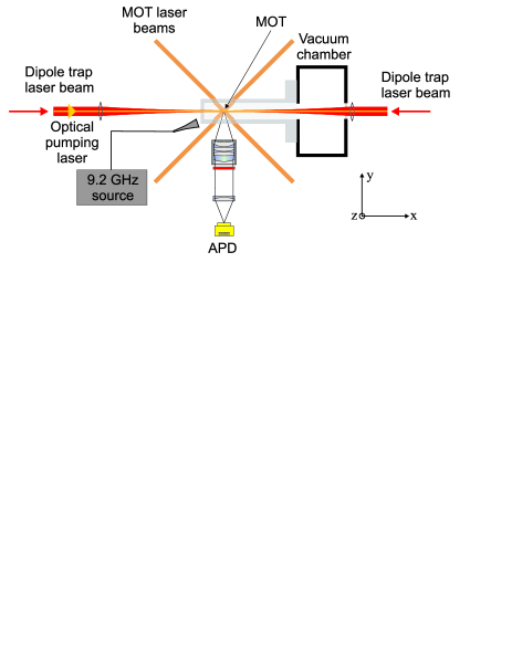
Figure 1: Experimental setup.

We trap and manipulate cesium atoms in a red detuned standing wave dipole trap. Our trap is formed of two counterpropagating Gaussian laser beams with waist $2w_{0}=40$ µm and a power of max. 2 W per beam (see Fig. 1), derived from a single Nd:YAG laser ($\lambda=1064$ nm). Typical trap depths are on the order of $U_{0}=1$ mK. The laser beams have parallel linear polarization and thus produce a standing wave interference pattern. Both laser beams are sent through acousto-optic modulators (AOMs), to mutually detune them for the realization of a moving standing wave. This “optical conveyor-belt” was introduced in previous experiments Kuhr01 ; Schrader01 and has been used for the demonstration of quantum state transportation Kuhr03 . For the experiments in this paper, however, we do not transport the trapped atoms. To eliminate any heating effect arising due to the phase noise of the AOM drivers Schrader01 ; Alt02b , we used the non-deflected beams (0^th order of the AOMs) to form the dipole trap. The AOMs are only used to vary the dipole trap laser intensity by removing power from the trap laser beams.

Cold atoms are loaded into the dipole trap from a high gradient magneto-optical trap (MOT). The high field gradient of the MOT ($\partial B/\partial z=340$ G/cm) is produced by water cooled magnetic coils, placed at a distance of 2 cm away from the trap. The magnetic field can be switched to zero within 60 ms (limited by eddy currents in the conducting materials surrounding the vacuum chamber) and it can be switched back on within 30 ms. Our vacuum chamber consists of a glass cell, with the cesium reservoir being separated from the main chamber by a valve. Cesium atoms are loaded into the MOT at random from the background gas vapor. To speed up the loading process, we temporarily lower the magnetic field gradient to $\partial B/\partial z=25$ G/cm during a time $t_{\rm low}$. The low field gradient results in a larger capture cross section which significantly increases the loading rate. Then, the field gradient is returned to its initial value, confining the trapped atoms at the center of the MOT. Varying $t_{\rm low}$ enables us to select a specific average atom number ranging from 1 to 50. The required time depends on the cesium partial pressure, which was kept at a level such that we load typically 50 atoms within $t_{\rm low}=100$ ms in these experiments.

In order to transfer cold atoms from the MOT into the dipole trap, both traps are simultaneously operated for some tens of milliseconds before we switch off the MOT. After an experiment in the dipole trap the atoms are transferred back into the MOT by the reverse procedure. All our measurements rely on counting the number of atoms in the MOT before and after any intermediate experiment in the dipole trap. For this purpose we collect their fluorescence light by a home-built diffraction-limited objective Alt02a and detect the photons with an avalanche photodiode (APD).

Three diode lasers are employed in this experiment which are set up in Littrow configuration and locked by polarization spectroscopy. The MOT cooling laser is stabilized to the $F=4\rightarrow F\mbox{${}^{\prime}$}=3/F\mbox{${}^{\prime}$}=5$ crossover transition and shifted by an AOM to the red side of the cooling transition $F=4\rightarrow F\mbox{${}^{\prime}$}=5$. The MOT repumping laser is locked to the $F=3\rightarrow F\mbox{${}^{\prime}$}=4$ transition, it is $\pi$-polarized and is shined in along the dipole trap axis. To optically pump the atoms into the $\left|\,F=4,m_{F}=0\,\right\rangle$ state, we use the unshifted MOT cooling laser, which is only detuned by +25 MHz from the required $F=4\rightarrow F\mbox{${}^{\prime}$}=4$ transition. This small detuning is partly compensated for by the light shift of the dipole trap. We shine in the laser along the dipole trap axis with $\pi$-polarization together with the MOT repumper. We found that 80% of the atoms are pumped into the $\left|\,F=4,m_{F}=0\,\right\rangle$ state, presumably limited by polarization imperfections of the optical pumping lasers.

For the state selective detection (see below) we use a “push-out” laser, resonant to the $F=4\rightarrow F\mbox{${}^{\prime}$}=5$ transition. It is $\sigma^{+}$-polarized and shined in perpendicular to the trapping beams (z-axis in Fig. 1).

To generate microwave pulses at the frequency of 9.2 GHz we use a synthesizer (Agilent 83751A), which is locked to an external rubidium frequency standard (Stanford Research Systems, PRS10). The amplified signal ($P=+36~{}\mbox{dBm}=4.0$ W) is radiated by a dipole antenna, placed at a distance 5 cm away from the MOT.

Compensation of the earth’s magnetic field and stray fields created by magnetized objects close to the vacuum cell is achieved with three orthogonal pairs of coils. For the compensation, we minimize the Zeeman splitting of the hyperfine ground state $m_{F}$ manifold which is probed by microwave spectroscopy. Using this method we achieve residual fields of $B_{\rm res}<0.4$ µT (4 mG). The coils of the $z$-axis also serve to produce a guiding field, which defines the quantization axis.

II.2 State selective detection of a single neutral atom

Sensitive experimental methods had to be developed in order to prepare and to detect the atomic hyperfine state at the level of a single atom. State selective detection is performed by a laser which is resonant with the $F=4\rightarrow F^{\prime}=5$ transition and thus pushes the atom out of the dipole trap if and only if it is in $F=4$. An atom in the $F=3$ state, however, is not influenced by this laser. Thus, it can be transferred back into the MOT and be detected there. Although this method appears complicated at first, it is universal, since it works with many atoms as well as with a single one. Other methods, such as detecting fluorescence photons in the dipole trap by illuminating the atom with a laser resonant to the $F=4\rightarrow F\mbox{${}^{\prime}$}=5$ transition, failed in our case because the number of photons detected before the atom decays into the $F=3$ state is not sufficient.

In order to achieve a high efficiency of the state selective detection process, it is essential to remove the atom out of the dipole trap before it is off-resonantly excited to $F\mbox{${}^{\prime}$}=4$ and spontaneously decays into the $F=3$ state. For this purpose, we use a $\sigma^{+}$-polarized push-out laser, such that the atom is optically pumped into the cycling transition $\left|\,F=4,m_{F}=4\,\right\rangle\rightarrow\left|\,F\mbox{${}^{\prime}$}=5,m_{F}=5\,\right\rangle$. In our setup, the polarization is not perfectly circular, since for technical reasons we had to shine in the laser beam at an angle of $2^{\circ}$ with respect to the magnetic field axis. This entails an increased probability of exciting the $F^{\prime}=4$ level from where the atom can decay into the $F=3$ ground state. To prevent this, we remove the atom from the trap sufficiently fast by shining in the push-out laser from the radial direction with high intensity ($I/I_{0}\approx 100$, with $w_{0}=100$ µm, $P=30$ µW, where $I_{0}=1.1$ mW/cm² is the saturation intensity). In this regime its radiation pressure force is stronger than the dipole force in the radial direction, such that we push out the atom within half the radial oscillation period ($\approx~{}1$ ms). In this case, the atom receives a momentum corresponding to the sum of all individual photon momenta. This procedure is more efficient than heating an atom out of the trap, which occurs when the radiation pressure force of the push-out laser is weaker than the dipole force, and the atom performs a random walk in momentum space while absorbing and emitting photons.

If we adiabatically lower the trap to typically $0.12$ mK prior to the application of the push-out laser, we need on average only 35 photons to push the atom out of the trap. This number is small enough to prevent off-resonant excitation to $F\mbox{${}^{\prime}$}=4$ and spontaneous decay to $F=3$.

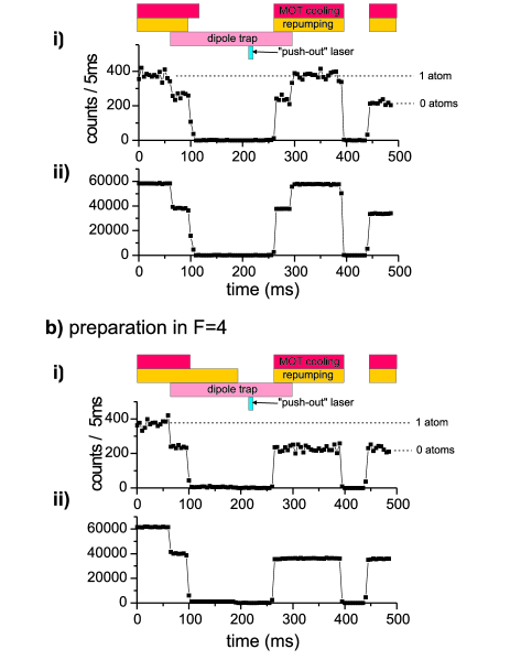
Figure 2: State selective detection of a single atom. The graphs show the fluorescence signal of the atom during state preparation and detection, binned in time intervals of 5 ms. The bars above the graphs show the timing of the lasers. Graphs (a)(i) and (b)(i) show the signals of a single atom, prepared in $F=3$ and $F=4$, respectively. Graphs (a)(ii) and (b)(ii) show the added signal of about 150 events.

A typical experimental sequence to test the state selective detection is shown in Fig. 2. First, the atom is transferred from the MOT into the optical dipole trap. Using the cooling and repumping laser of the MOT, we optically pump the atom either in the $F=3$ (Fig. 2a) or the $F=4$ hyperfine state (Fig. 2b). The push-out laser then removes all atoms in $F=4$ from the trap. Any remaining atom in $F=3$ is transferred back into the MOT, where it is detected.

Figures 2a(i) and 2b(i) show the signals of a single atom, prepared in $F=3$ and $F=4$, respectively. Our signal-to-noise ratio enables us to unambiguously detect the surviving atom in $F=3$, demonstrating the state-selective detection at the single atom level. We performed 157 repetitions with a single atom prepared in $F=3$ and found that in 153 of the cases the atom remains trapped, yielding a detection probability of $97.5^{+1.2}_{-2.0}\%$. Similarly, only 2 out of 167 atoms prepared in $F=4$ remain trapped, yielding 1.2${}^{+1.6}_{-0.8}\%$. The asymmetric errors are the Clopper-Pearson 68% confidence limits Barlow . These survival probabilities can also be inferred by directly adding the signals of the individual repetitions and by comparing the initial and final fluorescence levels in the MOT, see Figs. 2a(ii) and 2b(ii).

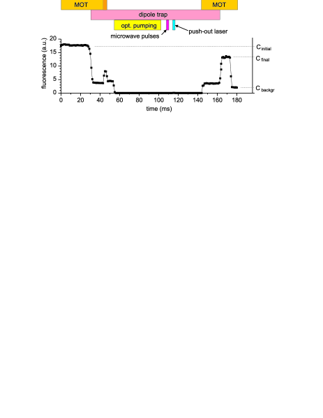
Figure 3: Atom counting. Initial and final numbers of atoms are inferred from their fluorescence in the MOT. Shown are the integrated APD counts binned in time intervals of 1 ms and accumulated over 10 repetitions with 20 atoms each.

All following experiments are performed in the same way. We initially prepare the atoms in the $\left|\,F=4,m_{F}=0\,\right\rangle$ state and measure the population transfer to $\left|\,F=3,m_{F}=0\,\right\rangle$ induced by the microwave radiation. After the application of one or a sequence of microwave pulses, the atom is in general in a superposition of both hyperfine states,

$$\left|\,\psi\,\right\rangle=c_{3}\left|\,F=3,m_{F}=0\,\right\rangle+c_{4}\left|\,F=4,m_{F}=0\,\right\rangle,$$ (1)

with complex probability amplitudes $c_{3}$ and $c_{4}$. Our detection scheme only allows us to measure the population of the hyperfine state $F=3$:

$$P_{3}=|c_{3}|^{2}=\frac{w+1}{2},$$ (2)

where $w$ is the third component of the Bloch vector, see below. The number $P_{3}$ is determined from the number of atoms before ($N_{\rm initial}$) and after ($N_{\rm final}$) any experimental procedure in the dipole trap. $N_{\rm initial}$ and $N_{\rm final}$ are inferred from the measured photon count rates, $C_{\rm initial}$, $C_{\rm final}$ and $C_{\rm backgr}$ (see Fig. 3):

$$N_{\rm initial}=\frac{C_{\rm initial}-C_{\rm backgr}}{C_{\rm 1atom}}$$ (3)

and

$$N_{\rm final}=\frac{C_{\rm final}-C_{\rm backgr}}{C_{\rm 1atom}}.$$ (4)

The fluorescence rate of a single atom, $C_{\rm 1atom}$, is measured independently. From the atom numbers we obtain the fraction of atoms transferred to $F=3$,

$$P_{3}=\frac{N_{\rm final}}{N_{\rm initial}}$$ (5)

The measured number of atoms, $N_{\rm inital}$ can be larger than the actual number of atoms in the dipole trap, since we lose atoms during the transfer from the MOT into the dipole trap (see below).

II.3 Rabi oscillations

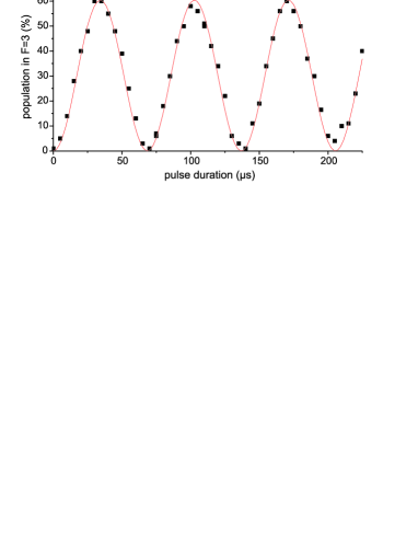
Figure 4: Rabi oscillations on the $\left|\,F=4,m_{F}=0\,\right\rangle\rightarrow\left|\,F=3,m_{F}=0\,\right\rangle$ clock transition recorded at a trap depth $U_{0}=1.0$ mK. Each data point results from 100 shots with about 60 initial atoms. The line is a fit according to Eq. (6).

We induce Rabi oscillations by a single resonant microwave pulse at the maximum RF power. For the graph of Fig. 4 we varied the pulse length from 0 µs to 225 µs in steps of 5 µs. Each point in the graph results from 100 shots with about $60\pm 10$ atoms each. The corresponding statistical error is below 1% and is thus not shown in the graph. The error of the data points in Fig. 4 is dominated by systematic drifts of the storage probability and efficiencies of the state preparation and detection. Since $w(t)=-\cos{\Omega_{\rm R}t}$, we fit the graph with

$$P_{\rm 3}(t)=\dfrac{C}{2}\left(1-\cos\Omega_{\rm R}t\right),$$ (6)

which yields a Rabi frequency $\Omega_{\rm R}/2\pi=(14.60\pm 0.02)$ kHz. Note that this Rabi frequency is higher than the one used later in this report (10 kHz) because we changed the position of the microwave antenna for practical reasons. The maximum population detected in $F=3$ is $C=(60.4\pm 0.7)$%. This reduction from 100% is caused by two effects. First, when we use many ($>40$) atoms at a time, up to 20% of the atoms are lost during the transfer from the MOT into the dipole trap due to inelastic collisions, as verified in an independent measurement. The remaining losses arise due to the non-perfect optical pumping process.

III Phenomenological description of decoherence and dephasing

In our experiment we observe quantum states in an ensemble average, and decoherence manifests as a decay or dephasing of the induced magnetic dipole moments. It is useful to distinguish between homogeneous and inhomogeneous effects. Whereas homogeneous dephasing mechanisms affect each atom in the same way, inhomogeneous dephasing only appears when observing an ensemble of many atoms possessing slightly different resonance frequencies. As we will see later, the most important difference between the two mechanisms is the fact that inhomogeneous dephasing can be reversed, in contrast to the irreversible homogeneous dephasing.

The interaction between the oscillating magnetic field component of the microwave radiation, $B\cos{\omega t}$, and the magnetic dipole moment, $\mu$, of the atom is well approximated by the optical Bloch equations AllenEberly :

$$\dot{\boldsymbol{u}}=-\boldsymbol{\Omega}\times\boldsymbol{u}$$ (7)

with the torque vector $\boldsymbol{\Omega}\equiv(\Omega_{\rm R},0,\delta)$ and the Bloch vector $\boldsymbol{u}\equiv(u,v,w)$. Here, $\Omega_{\rm R}=\mu B/\hbar$ is the Rabi frequency and $\delta=\omega-\omega_{0}$ is the detuning of the microwave from the atomic transition frequency $\omega_{0}$. In the following, the initial quantum state $\left|\,F=4,m_{F}=0\,\right\rangle$ corresponds to the Bloch vector $\boldsymbol{u}=(0,0,-1)$, whereas $\left|\,F=3,m_{F}=0\,\right\rangle$ corresponds to $\boldsymbol{u}=(0,0,1)$.

We include the decay rates as damping terms into the Bloch equations and use a notation of the different times for population and polarization decay similar to the one of nuclear magnetic resonance:

$$\dot{\left<u\right>} = \delta\left<v\right>-\frac{\left<u\right>}{T_{2}}$$ (8a)

$$\dot{\left<v\right>} = -\delta\left<u\right>+\Omega_{\rm R}\left<w\right>-\frac{\left<v\right>}{T_{2}}$$ (8b)

$$\dot{\left<w\right>} = -\Omega_{\rm R}\left<v\right>-\frac{\left<w\right>-w_{\rm st}}{T_{1}},$$ (8c)

where $\left<\dotsc\right>$ denotes the ensemble average. The total homogeneous transverse decay time $T_{2}$ is given by the polarization decay time $T_{2}\mbox{${}^{\prime}$}$ and the reversible dephasing time $T_{2}^{*}$

$$\frac{1}{T_{2}}=\frac{1}{T_{2}\mbox{${}^{\prime}$}}+\frac{1}{T_{2}^{*}}.$$ (9)

Inhomogeneous dephasing ($T_{2}^{*}$) occurs because the atoms may have different resonance frequencies depending on their environment. Thus the Bloch vectors of the individual atoms precess with different angular velocities and lose their phase relationship, they dephase. In our case, inhomogeneous dephasing arises due to the energy distribution of the atoms in the trap. This results in a corresponding distribution of light shifts because hot and cold atoms experience different average trapping laser intensities.

The longitudinal relaxation time, $T_{1}$, describes the population decay to a stationary value $w_{\rm st}$. In our case, $T_{1}$ is governed by the scattering of photons from the dipole trap laser, which couples the two hyperfine ground states via a two-photon Raman transition. This effect is suppressed due to a destructive interference effect yielding relaxation times of several seconds (see Sec. V.2). We do not include losses of atoms from the trap in the decay constants, which occur on the same timescale.

IV Inhomogeneous dephasing

We measure the transverse decay time $T_{2}$ by performing Ramsey spectroscopy, which consists of the application of two coherent rectangular microwave pulses, separated by a time interval $t$ Ramsey . The initial Bloch vector $\boldsymbol{u}_{0}=(0,0,-1)$ corresponds to an atom prepared in the $\left|\,F=4,m_{F}=0\,\right\rangle$-state. A $\pi/2$-pulse rotates the Bloch vector into the state $(0,-1,0)$, where the atom is in a superposition of both hyperfine states. The Bloch vector freely precesses in the $uv$-plane with an angular frequency $\delta$. Note that $\delta$ has to be small compared to the Rabi frequency and the spectral pulse width, such that the pulse can be approximated as near resonant, and complete population transfer can occur. After a free precession during $t$, a second $\pi/2$-pulse is applied. The measurement of the quantum state finally projects the Bloch vector onto the $w$ axis.

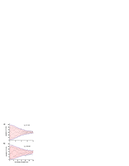
Figure 5: Ramsey fringes recorded for two different trap depths (a) $U_{0}=0.1$ mK and (b) $0.04$ mK. Their decay with time constants $T_{2}^{*}=4.4\pm 0.1$ ms and $20.4\pm 1.1$ ms, respectively, is governed by inhomogeneous dephasing caused by the energy distribution in the trap. Each data point results from 30 shots with about 50 initial atoms. The damped oscillation is a fit with $P_{\rm 3,Ramsey}(t)$ and the envelopes are the functions $B\pm A\alpha(t,T_{2}^{*})$ (see Eqs. (26), (29)).

We recorded Ramsey fringes for two different dipole trap depths, $U_{0}=0.1$ mK and $0.04$ mK (see Fig. 5). Each point in the graph of Fig. 5 corresponds to 30 shots with about 50 trapped atoms per shot, yielding errors (not shown) of less than 1%. The quoted values for $U_{0}$ are calculated from the measured power and the waist of the dipole trap laser beam and have an estimated uncertainty of up to 50%. We initially transfer the atoms from the MOT into a deeper trap ($U_{0}>1$ mK) to achieve a high transfer efficiency. When the MOT is switched off, we adiabatically lower the trap depth using the AOMs.

Our Ramsey fringes show a characteristic decay, which is not exponential. This decay is due to inhomogeneous dephasing, which occurs because after the first $\pi/2$-pulse, the atomic pseudo-spins precess with different angular frequencies. In the following, we derive analytic expressions for the observed Ramsey signal and we show that the envelope of the graphs of Fig. 5 is simply the Fourier transform of the atomic energy distribution.

IV.1 Differential light shift and decay of Ramsey fringes

The light shift of the ground state due to the Nd:YAG laser is simply the trapping potential

$$U_{0}(\Delta)=\frac{\hbar\Gamma}{8}\frac{I}{I_{0}}\frac{\Gamma}{\Delta}.$$ (10)

The detuning of the Nd:YAG-laser from the D-line of an atom in $F=4$ is 9.2 GHz less than for an atom in $F=3$. As a consequence, the $F=4$ level experiences a slightly stronger light shift, resulting in a shift of the $F=3\rightarrow F=4$ microwave transition towards smaller resonance frequencies. This differential light shift, $\delta_{0}$, can be approximated as

$$\hbar\delta_{\rm 0}=U_{0}(\Delta_{\rm eff})-U_{0}(\Delta_{\rm eff}+\omega_{\rm hfs}),$$ (11)

where $\Delta_{\rm eff}=-1.2\times 10^{7}~{}\Gamma$ is an effective detuning, taking into account the weighted contributions of the D₁ and D₂ lines Schrader01 . $\omega_{\rm hfs}=2.0\times 10^{3}~{}\Gamma$ is the ground state hyperfine splitting. Since $\omega_{\rm hfs}\ll\Delta_{\rm eff}$, we find that the differential light shift is proportional to the total light shift $U_{0}$,

$$\hbar\delta_{\rm 0}=\eta U_{0},$$ (12)

with a scaling factor $\eta=\omega_{\rm hfs}/\Delta_{\rm eff}=1.45\times 10^{-4}$. For atoms trapped in the bottom of a potential of $U_{0}=1$ mK, the differential light shift is $\delta_{0}=-2\pi\times 3.0$ kHz.

In the semiclassical limit, i. e. neglecting the quantized motion of the atom in the dipole trap potential, the free precession phase accumulated by an atomic superposition state between the two $\pi/2$-pulses depends on the average differential light shift only. In the following, we calculate the expected Ramsey signal using this semiclassical approach and obtain simple analytical expressions. Furthermore, we verified the validity of the presented model by performing a quantum mechanical density matrix calculation (not presented here) which agrees to within one percent with the semiclassical results. The small deviation can be attributed to the occurrence of small oscillator quantum numbers $n_{\rm osc}\simeq 5$ in the stiff direction of the trap.

Note that, strictly speaking, our model of a time-averaged differential light shift is only correct if the atom carries out an integer number of oscillation periods in the trap between the two $\pi/2$-pulses. However, we have checked that the variable phase accumulated during the remaining fraction of an oscillation period does not cause a measurable reduction of the Ramsey fringe contrast and can therefore be neglected.

Since a hot atom experiences a lower laser intensity than a cold one, its averaged differential light shift is smaller. The energy distribution of the atoms in the dipole trap obeys a three-dimensional Boltzmann distribution with probability density Metcalf ; korrMaxwell

$$p(E)=\frac{E^{2}}{2(k_{\rm B}T)^{3}}\,\exp{\left(-\frac{E}{k_{\rm B}T}\right)}.$$ (13)

Here $E=E_{\rm kin}+U$ is the sum of kinetic and potential energy. In a harmonic trap the virial theorem states that the average potential energy is half the total energy, $U=E/2$. Thus, the average differential light shift for an atom with energy $E$ is given by:

$$\delta_{\rm ls}(E)=\delta_{0}+\frac{\eta E}{2\hbar}$$ (14)

where $\delta_{0}<0$ is the maximum differential light shift. As a consequence, the energy distribution $p(E)$ yields, except for a factor and an offset, an identical distribution $\tilde{\alpha}(\delta_{\rm ls})$ of differential light shifts korrMaxwell :

$$\tilde{\alpha}(\delta_{\rm ls})=\frac{K^{3}}{2}(\delta_{\rm ls}-\delta_{\rm 0})^{2}\exp{[-K(\delta_{\rm ls}-\delta_{\rm 0})]}$$ (15)

with

$$K=\frac{2\hbar}{\eta k_{\rm B}T}.$$ (16)

Note that this distribution is only valid in the regime $k_{\rm B}T\ll U_{0}$, since the virial theorem was applied for the case of a harmonic potential.

To model the action of the Ramsey pulse sequence, we express the solutions of Eq. (7) as rotation matrices acting on the Bloch vector. The Ramsey sequence then reads

$$\boldsymbol{u}_{\rm Ramsey}(t)=\Theta_{\pi/2}\cdot\Phi_{\rm free}(\delta,t)\cdot\Theta_{\pi/2}\cdot\boldsymbol{u}_{0},$$ (17)

with the matrices describing the action of a $\pi/2$-pulse,

$$\Theta_{\pi/2}=\begin{pmatrix}1&0&0\\ 0&0&1\\ 0&-1&0\ \end{pmatrix},$$ (18)

and the free precession around the $w$-axis with angular frequency $\delta$ during a time interval $t$,

$$\Phi_{\rm free}(\delta,t)=\begin{pmatrix}\ \,\,\,\cos\phi(\delta,t)&\sin\phi(\delta,t)&0\\ -\sin\phi(\delta,t)&\cos\phi(\delta,t)&0\\ 0&0&1\ \end{pmatrix}.$$ (19)

The total precession angle, $\phi(\delta,t)$, represents the accumulated phase during the free evolution of the Bloch vector, $\phi(t)=\int_{0}^{t}\delta(t^{\prime})dt^{\prime}$. The detuning $\delta(t)$ may in general vary spatially and in time, depending on the energy shifts of the atomic levels.

If the Bloch vector is initially in the state $\boldsymbol{u}_{0}=(0,0,-1)$, we obtain from Eq. (17):

$$w_{\rm Ramsey}(t)=\cos\delta t,$$ (20)

where $\delta=\omega-\omega_{0}$ is the detuning of the microwave radiation with frequency $\omega$ from the atomic resonance $\omega_{0}$. In order to see the Ramsey fringes, we purposely shift $\omega$ with respect to the ground state hyperfine splitting, $\omega_{\rm hfs}$, by a small detuning, $\delta_{\rm synth}$, set at the frequency synthesizer

$$\omega=\omega_{\rm hfs}+\delta_{\rm synth}.$$ (21)

The atomic resonance frequency $\omega_{0}$ is modified due to external perturbations

$$\omega_{0}=\omega_{\rm hfs}+\delta_{\rm ls}+\delta_{\rm B},$$ (22)

where $\delta_{\rm ls}$ is the energy dependent differential light shift, $\delta_{\rm B}$ is the quadratic Zeeman shift.

Now, the inhomogeneously broadened Ramsey signal is obtained by averaging over all differential light shifts $\delta_{\rm ls}$:

$$\begin{array}[]{ll}\!\!\!\!\!\!w_{\rm Ramsey,inh}(t)=&\displaystyle\!\!\!\int^{\infty}_{\delta_{\rm 0}}\!\!\!\tilde{\alpha}(\delta_{\rm ls})\\ &\!\!\!\times\cos\left[(\delta_{\rm synth}-\delta_{\rm B}-\delta_{\rm ls})t\right]d\delta_{\rm ls}.\end{array}\vspace{0.2cm}$$ (23)

Eq. (23) shows that the shape of the Ramsey fringes is the Fourier(-Cosine)-Transform of the atomic energy distribution. Note that in the above integral we have set the upper integration limit to $\infty$, instead of the maximum physically reasonable value, $\delta_{0}/2$, to obtain the analytic solution

$$w_{\rm Ramsey,inh}(t)=\alpha(t,T_{2}^{*})\,\cos{\left[\delta\mbox{${}^{\prime}$}t+\kappa(t,T_{2}^{*})\right]},$$ (24)

with the sum of the detunings,

$$\delta\mbox{${}^{\prime}$}=\delta_{\rm synth}-\delta_{\rm B}-\delta_{\rm 0}$$ (25)

and a time- dependent amplitude $\alpha(t,T_{2}^{*})$ and phase shift $\kappa(t,T_{2}^{*})$ korrMaxwell

$$\alpha(t,T_{2}^{*})=\left[1+0.95\left(\frac{t}{T_{2}^{*}}\right)^{2}\right]^{-3/2}$$ (26)

and

$$\kappa(t,T_{2}^{*})=-3\arctan\left(0.97\frac{t}{T_{2}^{*}}\right).$$ (27)

Despite this non-exponential decay, we have introduced the inhomogeneous or reversible dephasing time $T_{2}^{*}$ as the 1/e-time of the amplitude $\alpha(t)$:

$$T_{2}^{*}=\sqrt{e^{2/3}-1}\,K=0.97\frac{2\hbar}{\eta k_{\rm B}T}.$$ (28)

Thus, the reversible dephasing time $T_{2}^{*}$ is inversely proportional to the temperature of the atoms.

The phase shift $\kappa(t,T_{2}^{*})$ arises due to the asymmetry of the probability distribution $\tilde{\alpha}(\delta_{\rm ls})$. The hot atoms in the tail of the energy distribution dephase faster than the cold atoms, due to their larger spread. The fact that these hot atoms no longer contribute to the Ramsey signal results in a weighting of the mean $\delta_{\rm ls}$ towards larger negative values.

To fit our experimental data, we derive the following expression from Eq. (24),

$$P_{\rm 3,Ramsey}(t) =B+\alpha(t,T_{2}^{*})$$ (29)

$$\times A\cos{\left[\delta\mbox{${}^{\prime}$}t+\kappa(t,T_{2}^{*})+\varphi\right]},$$

where the amplitude $A$ and the offset $B$ account for the imperfections of state preparation and detection. The other fit parameters are $\delta\mbox{${}^{\prime}$}$, $T_{2}^{*}$, and a phase offset $\varphi$.

	Fig. 5(a)				Fig. 5(b)
$U_{0}\mbox{ (est.)}$	0.1 mK				0.04 mK
$\delta_{\rm synth}/2\pi$	2250 Hz				1050 Hz
$A$	28.7	$\pm$	​​0.5	%	13.6	$\pm$	​​0.1	%
$B$	30.5	$\pm$	​​0.1	%	13.8	$\pm$	​​0.1	%
$\delta\mbox{${}^{\prime}$}/2\pi$	2133.7	$\pm$	​​1.5	Hz	722.5	$\pm$	​​0.5	Hz
$\varphi$	0.35	$\pm$	​​0.02		0.13	$\pm$	​​0.03
$T_{2}^{*}$	4.4	$\pm$	​​0.1	ms	20.4	$\pm$	​​0.6	ms

Table 1: Fit parameters extracted from the Ramsey fringes of Fig. 5 using Eq. (29).

The corresponding fits are shown in Fig. 5 and the resulting fit parameters are summarized in Table 1. For the two graphs, the maximum population detected in $F=3$, $P_{3,{\rm max}}=A+B$ is only about 60% and 30%, respectively. The reduction to 60% in Fig. 5(a) is again due to imperfections in the optical pumping process and due to losses by inelastic collisions, as discussed in Sec. II.3. The additional reduction in Fig. 5(b) occurs during the lowering of the trap to $U_{0}=0.04$ mK, where another 50% of the atoms are lost. Note, however, that the fringe visibility

$$V=\frac{A}{B}$$ (30)

is not impaired by these imperfections. From the fit parameters we obtain $V=0.97\pm 0.01$ and $V=1.00^{+0}_{-0.03}$ for the two cases.

As a check of consistency, we calculate the differential light shift $\delta_{0}$ from the fitted detuning $\delta\mbox{${}^{\prime}$}$ and the experimental values of $\delta_{\rm B}$ and $\delta_{\rm synth}$,

$$\delta_{0}=\delta_{\rm synth}-\delta_{\rm B}-\delta\mbox{${}^{\prime}$}.$$ (31)

The calculated quadratic Zeeman shift in the externally applied guiding field of $B=97.9\pm 1.5$ µT is $\delta_{\rm B}/2\pi=412\pm 13$ Hz, where the error is due to the uncertainty of the calibration. We obtain $\delta_{0}/2\pi=-268\pm 13$ Hz and $\delta_{0}/2\pi=-78\pm 13$ Hz. From the values of $\delta_{0}$ we can formally deduce the potential depth corresponding to $U_{0}=0.090\pm 0.004$ mK and $U_{0}=0.026\pm 0.004$ mK, which almost match the expected trap depths estimated from the dipole trap laser power assuming purely linear polarization. The discrepancy for the lowest trap depth could arise from the fact that the energy distribution is truncated at $E=U_{0}$, since we have lost the atoms with the highest energy during the lowering of the trap. This truncation will reduce the effective $\delta_{0}$ and thus yield a smaller trap depth.

Finally, the phase offset $\varphi$ occurs because the Bloch vector precesses around the $w$-axis even during the application of the two $\pi/2$-pulses. In contrast, our ansatz of Eq. (17) takes into account only the free precession in between the two pulses. The additional precession angle amounts to $\varphi=2\,t_{\pi/2}\,\delta\mbox{${}^{\prime}$}$. Given $t_{\pi/2}=16$ µs and the fitted value of $\delta\mbox{${}^{\prime}$}$ we obtain $\varphi=0.42$ for Fig. 5(a) and $\varphi=0.14$ for Fig. 5(b), which is close to the fitted values of Table 1.

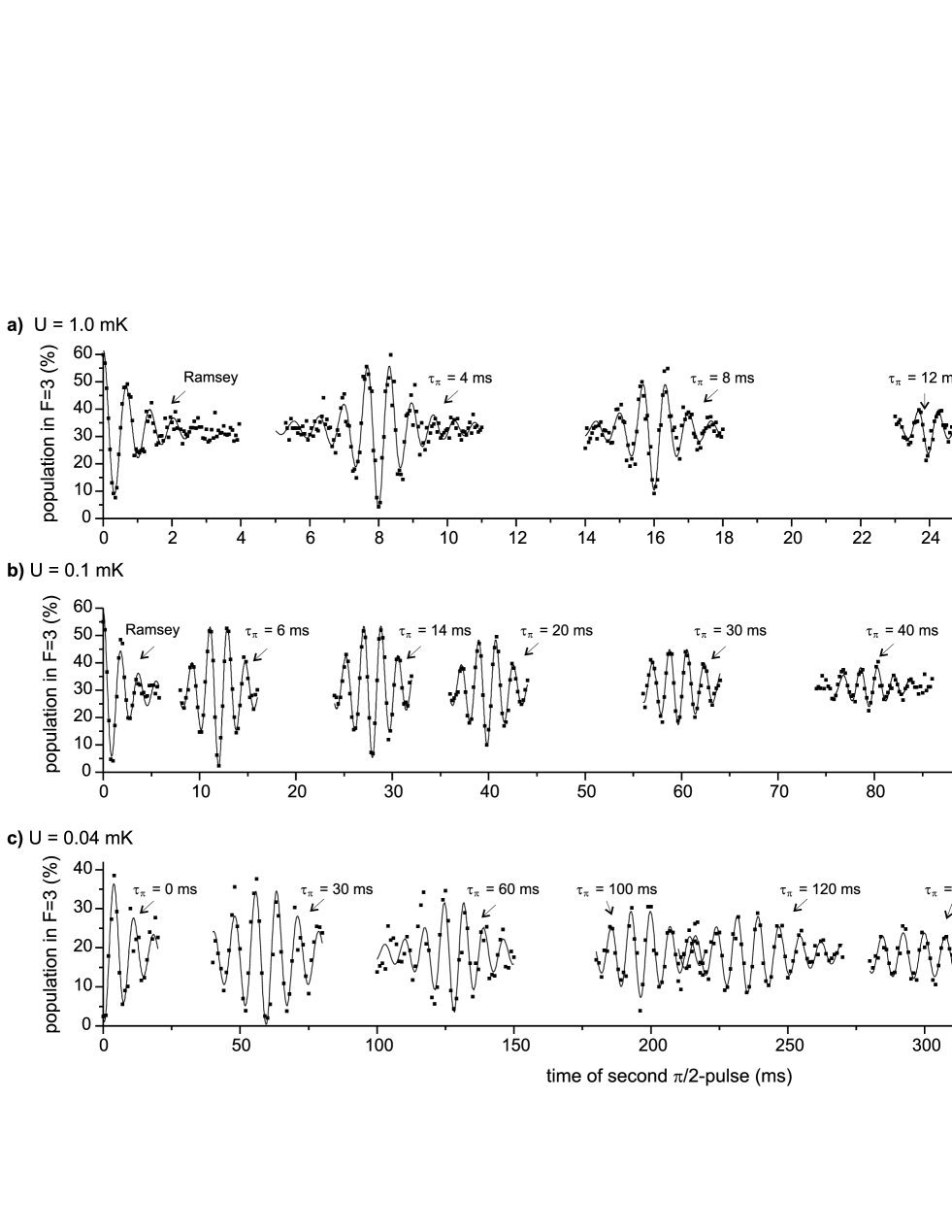
Figure 6: Spin echoes. Shown are spin echoes recorded for three different trap depths, (a) $U_{0}=1.0$ mK, (b) $0.1$ mK and (c) $0.04$ mK. We observe a decrease of the maximum spin echo amplitude with increasing time of the $\pi$-pulse, with longer decay times in lower trap depths. All spin echoes are fitted using Eq. (37). In (a) and (b), the first curve is a Ramsey signal, recorded with otherwise identical parameters.

V Homogeneous dephasing mechanisms

V.1 Spin echoes

The inhomogeneous dephasing can be reversed using a spin echo technique, i. e. by applying an additional $\pi$-pulse between the two Ramsey $\pi/2$-pulses. Although originally invented in the field of nuclear magnetic resonance Hahn50 , this technique was recently also employed in optical dipole traps Andersen03 .

We recorded echo signals in three different trap depths, $U_{0}=1.0$ mK, $0.1$ mK and $0.04$ mK for different times of the $\pi$-pulse, $\tau_{\pi}$ (see Fig. 6). We observe that the visibility of the echo signals decreases if we increase $\tau_{\pi}$. A slower decrease of the visibility is obtained in lower traps. For $U_{0}=0.04$ mK, $\tau_{\pi}=200$ ms, we even observed oscillations that reappear at $t=400$ ms.

In order to interpret these results, we first model the action of the microwave pulses for the spin echo, similar to the discussion in Sec. IV. After the first $\pi/2$-pulse at $t=0$, all Bloch vectors start at $\boldsymbol{u}(0)=(0,-1,0)$. Due to inhomogeneous dephasing, the Bloch vectors rotate at slightly different frequencies around the $w$-axis. A $\pi$-pulse at time $\tau_{\pi}$ rotates the ensemble of Bloch vectors around the $u$ axis by $180^{\circ}$ and induces a complete rephasing at $2\tau_{\pi}$ in the state $\boldsymbol{u}(2\tau_{\pi})=(0,1,0)$. The corresponding matrix equation reads

$$\boldsymbol{u}_{\rm echo}(t) = \Theta_{\pi/2}\cdot\Phi_{\rm free}(\delta,t-\tau_{\pi})\cdot\Theta_{\pi}\cdot$$ (32)

$$\cdot\Phi_{\rm free}(\delta,\tau_{\pi})\cdot\Theta_{\pi/2}\cdot\boldsymbol{u}_{0},$$

where we defined

$$\Theta_{\pi}=\begin{pmatrix}1&0&0\\ 0&-1&0\\ 0&0&-1\ \end{pmatrix}.$$ (33)

Here, $\tau_{\pi}$ is the time between the first $\pi/2$- and the $\pi$-pulse, and $t>\tau_{\pi}$ is the time of the second $\pi/2$ pulse. As a result of Eq. (32), we obtain

$$w_{\rm echo}(t)=-\cos[\delta(t-2\tau_{\pi})].$$ (34)

We calculate the shape of the inhomogeneously broadened echo signal, $w_{\rm echo,inh}(t)$, by integrating over all differential light shifts $\delta_{\rm ls}$

$$w_{\rm echo,inh}(t) = -\int^{\infty}_{\delta_{\rm 0}}\!\!\!\!\tilde{\alpha}(\delta_{\rm ls})\times$$ (35)

$$\times\cos\left[(\delta_{\rm synth}-\delta_{\rm ls}-\delta_{\rm B})(t-2\tau_{\pi})\right]d\delta_{\rm ls}.\rule[-19.91692pt]{19.91692pt}{0.0pt}$$

The integration yields a result similar to Eq. (23),

$$w_{\rm echo,inh}(t) = -\alpha(t-2\tau_{\pi})$$ (36)

$$\!\!\times\cos{\left[\delta\mbox{${}^{\prime}$}(t-2\tau_{\pi})+\kappa(t-2\tau_{\pi})\right]},$$

with amplitude $\alpha(t)$ and phase shift $\kappa(t)$ as defined in Eqs. (26) and (27). Eq. (36) shows that the amplitude of the echo signal regains its maximum at time $2\tau_{\pi}$. Finally, the population in $F=3$ reads:

$$P_{3,\rm echo}(t) = B-\alpha(t-2\tau_{\pi},T_{2}^{*})$$ (37)

$$\times A\cos{\left[\delta\mbox{${}^{\prime}$}(t\!-2\tau_{\pi})+\kappa(t-2\tau_{\pi},T_{2}^{*})+\psi\right]}.$$

This equation is used to extract dephasing times $T_{2}^{*}$ from all spin echoes of Fig. 6. The average values are listed in Table 2, where $T_{2}^{*}$ was obtained by averaging over the respective datasets. From the amplitude, $A$, and offset, $B$, of each echo signal we calculate the visibility $V=A/B$, plotted in Fig. 7 as a function of $\tau_{\pi}$. The phase shift $\psi$ accounts for slow systematic phase drifts during the spin echo sequence.

	Fig. 6(a)				Fig. 6(b)				Fig. 6(c)
$U_{0}\mbox{ (est.)}$	1.0 mK				0.1 mK				0.04 mK
$T_{2}^{*}$	0.86	$\pm$	​​0.05	ms	2.9	$\pm$	​​0.1	ms	18.9	$\pm$	​​1.7	ms
$T_{2}\mbox{${}^{\prime}$}$	10.2	$\pm$	​​0.4	ms	33.9	$\pm$	​​1.0	ms	146.2	$\pm$	​​6.6	ms
$T_{1}$ (calc.)	8.6 s				86 s				220 s

Table 2: Summary of dephasing times. $T_{2}^{*}$ and $T_{2}\mbox{${}^{\prime}$}$ are obtained from the echo signals of Fig. 6. $T_{1}=\Gamma_{\rm Raman}^{-1}$ is calculated using Eq. (63).

So far, we considered the detuning as constant during the experimental sequence. We now include in our model a time-varying detuning, $\delta(t)$, in order to account for a stochastic variation of the precession angles of the Bloch vector,

$$\phi_{1}=\int_{0}^{\tau_{\pi}}\delta(t)\,dt\quad\mbox{and}\quad\phi_{2}=\int_{\tau_{\pi}}^{2\tau_{\pi}}\delta(t)\,dt,$$ (38)

before and after the $\pi$-pulse. The phase difference $\phi_{2}-\phi_{1}$ is expressed as a mean difference of the detuning,

$$\Delta\delta=\frac{\phi_{2}-\phi_{1}}{\tau_{\pi}}.$$ (39)

The Bloch vector at time $2\tau_{\pi}$, when the inhomogeneous dephasing has been fully reversed, reads

$$\boldsymbol{u}_{\rm echo}(\Delta\delta,2\tau_{\pi}) = \Theta_{\pi/2}\cdot\Phi_{\rm free}(\delta+\Delta\delta,\tau_{\pi})\cdot\Theta_{\pi}\cdot$$ (40)

$$\cdot\Phi_{\rm free}(\delta,\tau_{\pi})\cdot\Theta_{\pi/2}\cdot\boldsymbol{u}_{0},$$

which results in

$$w_{\rm echo}(\Delta\delta,2\tau_{\pi})=-\cos(\Delta\delta\,\tau_{\pi}).$$ (41)

For a Gaussian distribution of fluctuations with mean $\overline{\Delta\delta}=0$ and variance $\sigma(\tau_{\pi})^{2}$,

$$p_{\tau_{\pi}}(\Delta\delta)=\frac{1}{\sigma(\tau_{\pi})\sqrt{2\pi}}\exp{\left[-\frac{(\Delta\delta)^{2}}{2\sigma(\tau_{\pi})^{2}}\right]},$$ (42)

the average $w$-component of the Bloch vector is calculated,

$$w_{\rm echo,hom}(2\tau_{\pi}) = \int_{-\infty}^{\infty}-\cos\left(\Delta\delta\,\tau_{\pi}\right)\,p_{\tau_{\pi}}(\Delta\delta)\,d\Delta\delta$$ (43)

$$= \exp\left[-\tfrac{1}{2}\tau_{\pi}^{2}\sigma(\tau_{\pi})^{2}\right].$$

Thus, the spin-echo visibility, $V$, yields

$$V(2\tau_{\pi})=V_{0}\,\exp{\left[-\tfrac{1}{2}\tau_{\pi}^{2}\,\sigma(\tau_{\pi})^{2}\right]}.$$ (44)

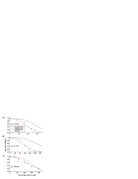
Figure 7: Decay of the spin echo visibility, extracted from the signals of Fig. 6. The fits (red lines) are the Gaussians of Eq. (45). The dashed and dotted lines are the best and worst case predictions inferred from the measured pointing instability of the trapping laser shown in Fig. 9.

For comparison with the experimental values, we fit the spin echo visibility of Fig. 7 with a Gaussian,

$$V(2\tau_{\pi})=C_{0}\exp{\left[-\frac{1}{2}\tau_{\pi}^{2}\sigma_{\rm exp}^{2}\right]}$$ (45)

with a time-independent detuning fluctuation $\sigma_{\rm exp}$. We define the homogeneous dephasing time $T_{2}\mbox{${}^{\prime}$}$ as the $1/e$ decay time of the spin echo visibility:

$$V(2T_{2}\mbox{${}^{\prime}$})=C_{0}e^{-1}\quad\Rightarrow\quad T_{2}\mbox{${}^{\prime}$}=\frac{\sqrt{2}}{\sigma_{\rm exp}}.$$ (46)

V.2 Origins of irreversible dephasing

Candidates for irreversible dephasing mechanisms include intensity fluctuations (1) and pointing instability of the dipole trap laser (2), heating of the atoms (3), fluctuating magnetic fields (4), fluctuations of the microwave power and pulse duration (5) and spin relaxation due to spontaneous Raman scattering from the dipole trap laser (6).

$U_{0}$

1.0 mK

0.1 mK

0.04 mK

$\sigma_{\rm exp}$ (meas.)

22.0

$\pm$

0.9

Hz

6.6

$\pm$

​​0.2

Hz

1.54

$\pm$

​​0.07

Hz

(1)

intensity fluctuations

$5.9$

Hz

$0.67$

Hz

$0.17$

Hz

pointing instability

(2)

best case

$10.6$

Hz

$2.4$

Hz

$1.3$

Hz

worst case

$21.6$

Hz

$6.7$

Hz

$3.7$

Hz

(3a)

heating $\sigma^{\rm(3)}_{\rm h}/2\pi$ (upper limit)

5.3

Hz

1.6

Hz

2.0

Hz

(3b)

photon scattering $\sigma_{\rm p}(T_{2}^{\prime})/2\pi$

4.5

Hz

1.5

Hz

1.4

Hz

(4)

magnetic field fluctuations $\sigma_{\rm b}(T_{2}\mbox{${}^{\prime}$})/2\pi$

1.7

Hz

0.35

Hz

0.17

Hz

Table 3: Summary of dephasing mechanisms. Shown are the fluctuation amplitudes $\sigma(T_{2}^{\prime})/2\pi$.

(1) Intensity fluctuations of the trapping laser. The intensity fluctuations are measured by shining the laser onto a photodiode and recording the resulting voltage as a function of time. From this signal we calculate $\sigma(\tau_{\pi})^{2}$ by means of the Allan variance, defined as Allan66 :

$$\sigma_{\rm A}^{2}(\tau)=\frac{1}{m}\sum_{k=1}^{m}\frac{(\overline{x}_{\tau,k+1}-\overline{x}_{\tau,k})^{2}}{2}.$$ (47)

Here $\overline{x}_{\tau,k}$ denotes the average of the photodiode voltages over the $k$-th time interval $\tau$, normalized to the mean voltage of the entire dataset. The resulting Allan deviation $\sigma_{\rm A}$ is a dimensionless number which expresses the relative fluctuations. They directly translate into fluctuations $\sigma(\tau)$ of the detuning,

$$\sigma(\tau)=\sqrt{2}\delta_{0}\sigma_{\rm A}(\tau).$$ (48)

The factor of $\sqrt{2}$ arises because $\sigma(\tau)$ is the standard deviation of the difference of two detunings with standard deviation $\sigma_{\rm A}(\tau)$ each. The maximum differential light shift $\delta_{0}$ in Eq. (48) is calculated according to Eq. (31) using the measured values of $\delta\mbox{${}^{\prime}$}$. As a result we find relative intensity fluctuations of $\sigma_{\rm A}(\tau)<0.2\%$ (see Fig. 8). The corresponding absolute fluctuation amplitudes $\sigma(T_{2}\mbox{${}^{\prime}$})/2\pi$ (shown in Table 3) are too weak to account for the observed decay of the spin echo visibility.

Figure 8: Allan deviation of the intensity fluctuations according to Eq. (47).

(2) Pointing instability of the trapping laser. Any change of the relative position of the two interfering laser beams also changes the interference contrast, and hence the light shift $\delta_{0}$. These position shifts can arise due to shifts of the laser beam itself, due to variations of the optical paths e. g. from acoustic vibrations of the mirrors or from air flow. In order to measure the pointing instabilities we mutually detune the two dipole trap beams by $\Delta\nu=10$ MHz using the AOMs and overlap them on a fast photodiode (see Fig. 9(a)). The amplitude of the resulting beat signal directly measures the interference contrast of the two beams and is thus proportional to the depth of the potential wells of the standing wave dipole trap. We used a network analyzer (HP 3589A) operated in “zero span” mode to record the temporal variation of the beat signal amplitude within a filter bandwidth of 10 kHz.

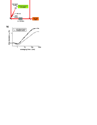
Figure 9: Measuring the pointing instability. (a) The dipole trap beams having a frequency difference of $\Delta\nu=10$ MHz are overlapped on a fast photodiode. (b) Allan deviation of the amplitude of the resulting beat signal.

The resulting Allan deviation of the beat signal amplitudes is shown in Fig. 9(b). The lower curve shows the signal in the case of well overlapped beams, whereas for the upper curve, we purposely misaligned the beams so that the beat signal amplitude is reduced by a factor of 2. In the latter case variations of the relative beam position cause a larger variation of the beat signal amplitude, since the beams overlap on the slopes of the Gaussian profile.

These two curves measure the best and the worst cases of the fluctuations. We found that the relative fluctuations for long time scales of $\tau>100$ ms reach up to 3% in the worst case. They are thus one order of magnitude greater than the variations caused by intensity fluctuations. The frequency fluctuations $\sigma(\tau)$ are again calculated using Eq. (48). This result is plotted together with the observed visibility in Fig. 7. Our data points lie in between these best and worst case predictions.

(3a) Heating effects. Heating processes in the trap can also cause significant irreversible decoherence, since they cause a variation of the atomic resonance frequency within the microwave pulse sequence. A constant heating rate $\dot{E}$ increases the average energy of the atoms for the second free precession interval $[\tau_{\pi},2\tau_{\pi}]$, compared to the first interval $[0,\tau_{\pi}]$, by $\dot{E}\tau_{\pi}$. The energy $E$ of individual atoms, however, can be changed by much more than this average energy gain.

To estimate the effect we have to calculate the typical energy change of individual atoms during the free precession interval caused by the fluctuating forces which are responsible for the heating. For this purpose we approximate the trap as harmonic and assume the following model of the heating process. Due to a random walk in momentum space, an initial atomic momentum $p=\sqrt{2mE}$ evolves into a symmetric, Gaussian momentum distribution around $p$ with a standard deviation of $\Delta p_{\rm rms}$ given by the average energy gain $\dot{E}\tau_{\pi}$

$$\dot{E}\tau_{\pi}=\frac{(\Delta p_{\rm rms})^{2}}{2m}.$$ (49)

Assuming $E\gg\dot{E}\tau_{\pi}$ we can linearly approximate the energy-momentum relationship at $E$. In this approximation the momentum distribution is therefore equivalent to a Gaussian distribution of the energies with

$$\Delta E_{\rm rms}=2\sqrt{E\dot{E}\tau_{\pi}}.$$ (50)

According to Eq. (14) the corresponding standard deviation $\sigma_{{\rm heat},E}$ of the detunings $\Delta\delta$ is

$$\sigma_{{\rm heat},E}(\tau_{\pi})=\frac{\eta}{\hbar}\sqrt{E\dot{E}\tau_{\pi}},$$ (51)

depending on the initial energy E.

We now integrate the distribution of the detunings

$$\!\!\!\!\!\!\!\!\!\!\!p_{E}(\Delta\delta)=$$

$$\!\!\!\!\!\!=\frac{1}{\sqrt{2\pi}}\frac{1}{\sigma_{{\rm heat},E}(\tau_{\pi})}\exp{\left(-\frac{\Delta\delta^{2}}{2\bigl{(}\sigma_{{\rm heat},E}(\tau_{\pi})\bigr{)}^{2}}\right)}$$ (52)

over the initial energy $E$ weighted by the $n$-dimensional thermal energy distribution $p^{(n)}(E)\propto E^{n-1}\exp{\left(-{E}/{k_{B}T}\right)}$:

$$p^{(n)}(\Delta\delta)=\int_{0}^{\infty}p_{E}(\Delta\delta)p^{(n)}(E)dE.$$ (53)

Finally we obtain the rms detuning fluctuations $\sigma_{\rm heat}$ from the resulting distribution of $\Delta\delta$ as

$$\left[\sigma^{(n)}_{\rm heat}(\tau_{\pi})\right]^{2}=\int_{-\infty}^{\infty}\Delta\delta^{2}p^{(n)}(\Delta\delta)d\Delta\delta.$$ (54)

Evaluation of $\sigma^{(n)}_{\rm heat}$ for the experimentally relevant time scale $\tau_{\pi}=T_{2}^{\prime}/2$ yields

$$\sigma^{(n)}_{\rm heat}=\frac{\eta}{\hbar}\sqrt{\frac{n}{2}\dot{E}T_{2}^{\prime}k_{B}T}.$$ (55)

Heating effects in our trap have been investigated in detail in Ref. Alt02b . An upper limit for the heating rate of $\dot{E}=2\cdot 10^{-2}$ mK/s is obtained from the trap lifetime of 50 s (for $U_{0}=1.0$ mK). When we linearly scale $\dot{E}$ to our trap depths of $U_{0}=1.0$ mK, $U_{0}=0.1$ mK, and $U_{0}=0.04$ mK, and assume temperatures of $T=0.1$ mK, $T=0.06$ mK, and $T=0.02$ mK, we obtain fluctuation amplitudes for the 3D-case ($n=3$) of $\sigma^{(3)}_{\rm heat}=5.3$ Hz, $\sigma^{(3)}_{\rm heat}=1.6$ Hz and $\sigma^{(3)}_{\rm heat}=2.0$ Hz, respectively. We stress however, that these values for $\sigma_{\rm heat}$ are upper limits since we did not measure heating rates $\dot{E}$ for the trap depths we used. The actual values of $\dot{E}$ and the resulting values for $\sigma_{\rm heat}$ could be orders of magnitude smaller than the upper limits inferred from the life time because the heating rate strongly depends on the oscillation frequencies and the details of the laser noise spectrum.

(3b) Photon recoil. Our model of the heating process also gives an estimate of the dephasing due to photon recoil. If we had one photon scattered per time interval $\tau_{\pi}$ giving two recoils, we would obtain a heating rate

$$\dot{E}=\frac{\hbar^{2}k^{2}}{m}\frac{1}{\tau_{\pi}}.$$ (56)

Inserting into Eq. (55) ($n=3$) yields

$$\sigma_{\rm heat}^{\rm 1ph}=\eta k\sqrt{\frac{3k_{B}T}{m}}.$$ (57)

Scattering of $n_{\rm ph}$ photons would yield

$$\sigma_{\rm ph}(n_{\rm ph})=\sqrt{n_{\rm ph}}\,\sigma_{\rm heat}^{\rm 1ph}.$$ (58)

Given a scattering rate $\Gamma_{\rm s}$, the number of scattered photons obeys a Poissonian distribution. Since for our parameters, the probability of scattering more than one photon is negligible, we obtain

$$\sigma_{\rm ph}(\tau_{\pi})=\eta k\sqrt{\frac{3k_{B}T\Gamma_{\rm s}\tau_{\pi}}{m}}\exp{\left(-\frac{\Gamma_{\rm s}\tau_{\pi}}{2}\right)}.$$ (59)

We use the temperatures of the previous paragraph and the photon scattering rates (see below) of $\Gamma_{\rm s}=10.6$ s^-1, $\Gamma_{\rm s}=1.06$ s^-1 and $\Gamma_{\rm s}=0.41$ s^-1. With $\tau_{\pi}=T_{2}^{\prime}/2$ we obtain $\sigma_{\rm ph}(T_{2}^{\prime})=4.5$ Hz, $\sigma_{\rm ph}(T_{2}^{\prime})=1.5$ Hz and $\sigma_{\rm ph}(T_{2}^{\prime})=1.4$ Hz, respectively.

(4) Fluctuating magnetic fields. Using a fluxgate magnetometer we measured a peak-to-peak value of the magnetic field fluctuations of $\Delta B=0.13~{}\mu$T, dominated by components at $\nu=50$ Hz. The resulting frequency shift on the $\left|\,F=4,m_{F}=0\,\right\rangle$ $\rightarrow$ $\left|\,F=3,m_{F}=0\,\right\rangle$ transition is:

$$\Delta\omega=2\,\Delta\omega_{0\rightarrow 0}\,B_{0}\,\Delta B,$$ (60)

where $B_{0}=97.9~{}\mu$T is the offset field and $\Delta\omega_{0\rightarrow 0}/2\pi=43$ mHz/($\mu$T)² is the quadratic Zeeman shift. For our case, we obtain $\Delta\omega=1.1$ Hz.

The effect of the magnetic fluctuations depends on the time interval between the microwave pulses. If this time is large compared to $1/\nu$, all fluctuations cancel except for those of the last oscillation period. As a consequence, the effect on the detuning fluctuations $\sigma$ also decreases. We calculate this effect by computing the Allan deviation $\sigma_{\rm A}(\tau)$ of a 50 Hz sine signal. The detuning fluctuations then read $\sigma_{\rm b}(\tau)=\sqrt{2}\Delta\omega\,\sigma_{\rm A}(\tau)$. The resulting $\sigma_{\rm b}(T_{2}\mbox{${}^{\prime}$})$, shown in Table 3, is too small to account for the decay of the spin echo amplitude.

(5) Fluctuation of microwave power and pulse durations. The application of two $\pi/2$-pulses and one $\pi$-pulse results in $w_{\rm echo}(2\tau_{\pi})=-1$. Any fluctuations of the amplitude ($\Delta\Omega_{\rm R}/\Omega_{\rm R}$) or pulse duration ($\Delta\tau/\tau$) result in variations of the amplitude of the spin echo signal, i. e. $w_{\rm echo}(2\tau_{\pi})=-\cos\Delta\phi$ according to:

$$\ \left(\frac{\Delta\phi}{2\pi}\right)^{2}=\left(\frac{\Delta\Omega_{\rm R}}{\Omega_{\rm R}}\right)^{2}+\left(\frac{\Delta\tau}{\tau}\right)^{2}$$ (61)

With $\Delta\tau/\tau<10^{-3}$ (measured) and $\Delta\Omega_{\rm R}/\Omega_{\rm R}<10^{-2}$ (specifications of the synthesizer) we obtain $\Delta\phi/2\pi<10^{-2}$, which is too small to be observed. Moreover, this effect neither depends on the dipole trap depth nor on the time delay between the microwave pulses.

The timing of the microwave pulses would be affected by a clock inaccuracy of the D/A-board of the computer control system which triggers the microwave pulses. Its specified accuracy $\Delta\tau/\tau=10^{-4}$, results in a phase fluctuation $\delta\mbox{${}^{\prime}$}\tau_{\pi}\,\Delta\tau/\tau<0.01$ for all parameters $\delta\mbox{${}^{\prime}$}$ and $\tau_{\pi}$ used in our experiment. Thus, the fluctuations of microwave power, pulse duration, and timing do not account for the observed reduction of the spin echo visibility.

(6) Spin relaxation due to light scattering. The population decay time, $T_{1}$, is governed by the scattering of photons from the dipole trap laser, which couples the two hyperfine ground states via a two-photon Raman transition. In our case, the hyperfine changing spontaneous Raman processes are strongly reduced due to a destructive interference of the transition amplitudes. Thus, the spin relaxation rate is much larger than the spontaneous scattering rate. This effect was first observed on optically trapped Rubidium atoms in the group of D. Heinzen Cline94 and was also verified in experiments in our group Frese00 .

The corresponding transition rate is calculated by means of the Kramers-Heisenberg formula Loudon , which is a result from second order perturbation theory. We obtain for the rate of spontaneous transitions, $\Gamma_{\rm s}$, from the ground state $\left|\,F,m\,\right\rangle$ to the ground state $\left|\,F^{\prime\prime},m^{\prime\prime}\,\right\rangle$:

$$\Gamma_{\rm s}=\frac{3c^{2}\omega_{\rm L}^{3}I}{4\hbar\,d^{4}}\left|\frac{a^{\mbox{\tiny(1/2)}}}{\Delta_{\rm 1/2}}+\frac{a^{\mbox{\tiny(3/2)}}}{\Delta_{\rm 3/2}}\right|^{2},$$ (62)

where $\Delta_{\rm J^{\prime}}=\omega_{\rm L}-\omega_{\rm J^{\prime}}$ is the detuning of the dipole trap laser from the ${}^{6}\!P_{\rm J^{\prime}}$-state and $d=\left\langle\,4,4\,\right|\mu_{+1}\left|\,5,5\,\right\rangle$, with the dipole operator $\mu_{+1}$ for $\Delta m=+1$ transitions. The transition amplitudes $a^{\mbox{\tiny(J')}}$ are obtained by summing over all possible intermediate states $\left|\,F^{\prime},m^{\prime}\,\right\rangle$ of the relevant ${}^{6}\!P_{\rm J^{\prime}}$ manifold Cline94 . For Rayleigh scattering processes, which do not change the hyperfine state ($F,M=F^{\prime\prime},M^{\prime\prime}$), the amplitudes add up, $a^{\mbox{\tiny(3/2)}}=2a^{\mbox{\tiny(1/2)}}$. However, for state changing Raman processes ($F,M\neq F^{\prime\prime},M^{\prime\prime}$), the two transition amplitudes are equal but have opposite sign, $a^{\mbox{\tiny(3/2)}}=-a^{\mbox{\tiny(1/2)}}$. Then the two terms in Eq. (62) almost cancel in the case of far detuning, $\Delta_{1/2}\approx\Delta_{3/2}$. As a result the spontaneous Raman scattering rate scales as $1/\Delta^{4}$ whereas the Rayleigh scattering rate scales as $1/\Delta^{2}$. The suppression factor can be expressed using the fine structure splitting $\Delta_{\rm fs}=\Delta_{\rm 3/2}-\Delta_{\rm 1/2}$ as

$$\Gamma_{\rm Raman}=\beta\,\Gamma_{\rm s}\qquad\mbox{with}\quad\beta=\left|\frac{\Delta_{\rm fs}}{3\Delta_{\rm 1/2}}\right|^{2}.$$ (63)

For the case of cesium, we obtain a suppression factor of $\beta=0.011$. The Rayleigh scattering rate for an atom trapped in a potential of $U_{0}=1.0$ mK is $\Gamma_{\rm s}=11$ s^-1. Then, the corresponding spontaneous Raman scattering rate is $\Gamma_{\rm Raman}=0.12$ s^-1 and the population decay time $T_{1}=\Gamma_{\rm Raman}^{-1}=8.6$ s. Since in most of our experiments, the trap depth is significantly smaller, $T_{1}$ will be even larger. As a consequence, we neglect the population decay due to spontaneous scattering. Note that the experiments of Refs. Cline94 ; Frese00 were only sensitive to changes of the hyperfine $F$-state, since the atoms were in a mixture of $m_{F}$-sublevels. However, the theoretical treatment above predicts similarly long relaxation times for any particular $m_{F}$-sublevel, which is consistent with our observations.

V.3 Conclusions

We have developed an analytical model which treats the various decay mechanisms of the hyperfine coherence of trapped cesium atoms independently. This is justified by the very different time scales of the decay mechanisms ($T_{2}^{*}\ll T_{2}\mbox{${}^{\prime}$}\ll T_{1}$). Our model reproduces the observed shapes of Ramsey and spin echo signals, whose envelopes are the Fourier transform of the energy distribution of the atoms in the trap.

The irreversible decoherence rates manifest themselves in the decay of the spin echo visibility and are caused by fluctuations of the atomic resonance frequency in between the microwave pulses. In the above analysis we have investigated various dephasing mechanisms and characterized them by the corresponding amplitude of the detuning fluctuations which are summarized in Table 3. We find that a major mechanism of irreversible dephasing is the pointing instability of the dipole trap laser beams resulting in fluctuations of the trap depth and thus the differential light shift. Significant decoherence is also caused in the shallow dipole trap by heating due to photon scattering. Heating due to technical origin, such as fluctuations of the depth and the position of the trap, cannot be excluded as an additional source of decoherence.

Compared to our experiment, significantly longer coherence times ($T_{2}^{*}=4$ s) were observed by N. Davidson and S. Chu in blue detuned traps in which the atoms are trapped at the minimum of electric fields Davidson95 . In Ref. Davidson95 , $T_{2}^{*}=15$ ms obtained with sodium atoms in a Nd:YAG dipole trap ($U_{0}=0.4$ mK) was reported, which is comparable to our observation. In other experiments, the inhomogeneous broadening has been reduced by the addition of a weak light field, spatially overlapped with the trapping laser field and whose frequency is tuned in between the two hyperfine levels Kaplan02 . Of course, cooling the atoms to the lowest vibrational level by using e. g. Raman sideband cooling techniques Hamann98 ; Perrin98 , would also reduce inhomogeneous broadening. The magnetic field fluctuations could possibly be largely suppressed by triggering the experiment to the 50 Hz of the power line.

- (1) W. H. Zurek, Phys. Rev. D 26, 1862 (1982).
- (2) W. H. Zurek, Physics Today 44, 36 (October 1991).
- (3) M. Brune et al., Phys. Rev. Lett. 77, 4887 (1996).
- (4) S. Haroche, Physics Today 51, 36 (July 1998).
- (5) C. Monroe, D. M. Meekhof, B. E. King and D. J. Wineland, Science 272, 1131 (1996).
- (6) F. Schmidt-Kaler et al., J. Phys. B: At. Mol. Opt. Phys. 36, 623 (2003).
- (7) N. Davidson, H. J. Lee, C. S. Adams, M. Kasevich and S. Chu, Phys. Rev. Lett. 74, 1311 (1995).
- (8) R. Ozeri, L. Khaykovich and N. Davidson, Phys. Rev. A 59, R1750 (1999).
- (9) S. Kuhr et al., Science 293, 278 (2001).
- (10) D. Schrader et al., Appl. Phys. B 73, 819 (2001).
- (11) S. Kuhr et al., Phys. Rev. Lett. 91, 213002 (2003).
- (12) W. Alt et al., Phys. Rev. A 67, 033403 (2003).
- (13) H. Metcalf, P. van der Straten, Laser Cooling and Trapping, Springer, 1st ed. (1999).
- (14) In Refs. Kuhr03 and Alt02b we erroneously used the energy distribution , valid for particles in free space. We now use the correct distribution of Eq. (13). This implies that Eqs. (1) and (3) of Ref. Kuhr03 have to be replaced by Eqs. (15) and (26) of this paper. Please see also the errata to Refs. Kuhr03 and Alt02b (to be published).
- (15) W. Alt, Optik 113, 142 (2002).
- (16) R. Barlow, Statistics, Wiley, New York (1989).
- (17) L. Allen, J. H. Eberly, Optical resonance and two-level atoms, Wiley, New York (1975).
- (18) N. Ramsey, Molecular Beams, Oxford University Press, London (1956).
- (19) E. Hahn, Phys. Rev. 80, 580 (1950).
- (20) M. F. Andersen, A. Kaplan, N. Davidson, Phys. Rev. Lett 90, 023001 (2003).
- (21) D. W. Allan, Proc. IEEE 54, 221 (1966).
- (22) R. A. Cline, J. D. Miller, M. R. Matthews, D. J. Heinzen, Opt. Lett. 19, 207 (1994).
- (23) D. Frese et al., Phys. Rev. Lett. 85, 3777 (2000).
- (24) R. Loudon, The Quantum Theory of Light, Clarendon, Oxford (1983).
- (25) A. Kaplan, M. F. Andersen, N. Davidson, Phys. Rev. A 66, 045401 (2002).
- (26) S. E. Hamann et al., Phys. Rev. Lett. 80, 4149 (1998).
- (27) H. Perrin, A. Kuhn, I. Bouchoule and C. Salomon, Europhys. Lett. 42, 395 (1998).