Entanglement, Bell Inequalities
and Decoherence in Particle Physics

Abstract

We demonstrate the relevance of entanglement, Bell inequalities and decoherence in particle physics. In particular, we study in detail the features of the “strange” $K^{0}\bar{K}^{0}$ system as an example of entangled meson–antimeson systems. The analogies and differences to entangled spin–$\frac{1}{2}$ or photon systems are worked out, the effects of a unitary time evolution of the meson system is demonstrated explicitly. After an introduction we present several types of Bell inequalities and show a remarkable connection to $CP$ violation. We investigate the stability of entangled quantum systems pursuing the question of how possible decoherence might arise due to the interaction of the system with its “environment”. The decoherence is strikingly connected to the entanglement loss of common entanglement measures. Finally, some outlook of the field is presented.

1 Introduction

In 1935, in his famous trilogy on “The present situation of quantum mechanics”, Erwin Schrödinger Schrodinger already realized the peculiar features of what he called entangled states —“…verschränkte Zustände…” was actually his German phrasing— in connection with quantum systems extended over physically distant parts. In the same year Einstein, Podolsky and Rosen (EPR) EPR constructed a gedanken experiment for a quantum system of two distant particles to demonstrate: Quantum mechanics is incomplete! Niels Bohr Bohr replied immediately to the EPR article. His message was: Quantum mechanics is complete!

Also in 1935, W.H. Furry Furry emphasized, inspired by EPR and Schrödinger, the differences between the predictions of quantum mechanics (QM) of non-factorizable systems and models with spontaneous factorization.

However, the EPR–Bohr debate was regarded as rather philosophical and thus not very valuable for physicists for about 30 years until John Stewart Bell bell brought this issue up again in his seminal work of 1964 “On the Einstein–Podolsky–Rosen Paradox”, which caused a dramatic change in the view about this subject. Bell discovered what has since become known as Bell’s Theorem:

• No local hidden variable theory can reproduce all possible results of QM !

It is achieved by establishing an inequality satisfied by the expectation values of all local realistic theories (LRT) but violated by the predictions of QM. Inequalities of this type are nowadays named quite generally Bell inequalities (BI).

It is the nonlocality arising from quantum entanglement —the “spooky action at distance” as we concluded in the 1980s Bertlmann — which is the basic feature of quantum physics and is so contrary to our intuition.

Many beautiful experiments have been carried out over the years (see e.g. Refs. FreedmanClauser ; FryThompson ; aspect ; WeihsZeilinger ) by using the entanglement of the polarization of two photons; all (also the long–distance GisinGroup or out-door experiments AspelmeyerZeilinger ) confirm impressively: Nature contains a spooky action at distance!

The nonlocality does not conflict with Einstein’s relativity, so it cannot be used for superluminal communication, nevertheless, Bell’s work bell ; bell2 initiated new physics, like quantum cryptography Ekert ; DeutschEkert ; Hughes ; GisinGroup and quantum teleportation Bennett-teleport ; ZeilingerTele , and it triggered a new technology: quantum information and quantum communication ZeilingerInfo1 ; ZeilingerInfo2 . More about “from Bell to quantum information” can be found in the book BertlmannZeilinger .

1.1 Particle physics

Of course, it is of great interest to investigate the EPR–Bell correlations of measurements also for massive systems in particle physics. Here we want to work out the analogies and differences to the spin–$\frac{1}{2}$ or photon systems. Already in 1960, Lee and Yang lee and several other authors Inglis ; Day ; Lipkin emphasized the EPR-like features of the “strange” $K^{0}\bar{K}^{0}$ system in a $J^{PC}=1^{--}$ state, where the quantum number strangeness $S=+,-$ plays the role of spin $\Uparrow$ or $\Downarrow$. Indeed many authors eberhard ; eberhard2 ; bigi ; domenico ; Bramon ; AncoBramon ; BramonGarbarino ; Genovese suggested to investigate the $K^{0}\bar{K}^{0}$ pairs which are produced at the $\Phi$ resonance, for instance in the $e^{+}e^{-}$–machine DA$\Phi$NE at Frascati. The nonseparability of the neutral kaon system —created in $p\bar{p}$–collisions— has been already analyzed by the authors of Refs. six ; CPLEAR-EPR ; BGH .

Similar systems are the entangled beauty mesons, $B^{0}\bar{B}^{0}$ pairs, produced at the $\Upsilon$(4S) resonance (see e.g., Refs. BG1 ; Dass ; BG2 ; datta ; selleribmeson ; BG3 ), which we touch only little in this Article.

Specific realistic theories have been constructed selleri ; SelleriBook ; six2 ; BramonGarbarino2 , which describe the $K^{0}\bar{K}^{0}$ pairs, as tests versus quantum mechanics. However, a general test of LRT versus QM relies on Bell inequalities, where —as we shall see— the different kaon detection times or the freely chosen kaon “quasi–spin” play the role of the different angles in the photon or spin–$\frac{1}{2}$ case. Furthermore, an interesting feature of kaons (and also of B–mesons) is $CP$ violation (charge conjugation and parity) and indeed it turns out that BI imply bounds on the physical $CP$ violation parameters.

The important difference of the kaon systems as compared to photons is their decay. We emphasize the necessity of including also the decay product states into the BI in order to have a unitary time evolution BertlmannHiesmayr2001 .

A main part of the article is also devoted to the investigation of the stability of the entangled quantum system. How possible decoherence might arise from the interaction of the system with its “environment”, whatever this may be, and we will determine the strength of such effects. We study how decoherence is related to the loss of entanglement, and pursue the question: how to detect and quantify entanglement BertlmannDurstbergerHiesmayr2002 .

Of course, we cannot cover all subjects of the field. In Section 10 we mention interesting works we could not describe here and give an outlook to what we can expect in the near future.

Thus the contents of our article will be briefly the following:

• QM of K–mesons

• Introduction to BI

• BI for $K$-mesons, in time and “quasi–spin”

• Decoherence in entangled $K^{0}\bar{K}^{0}$ system

• Entanglement measures, entanglement loss and decoherence

2 QM of $K$–mesons

Neutral K–mesons are wonderful quantum systems! Four phenomena illustrate their “strange” behavior that is associated with the work of Abraham Pais GellMannPais ; PaisPiccioni :

1. strangeness

2. strangeness oscillation

3. regeneration

4. $CP$ violation.

Let us start with a discussion of the properties of the neutral kaons, which we need in the following.

2.1 Strangeness

$K$-mesons are characterized by their strangeness quantum number $S$

$$S|K^{0}\rangle\; = +|K^{0}\rangle\;,$$

$$S|\bar{K}^{0}\rangle\; = -|\bar{K}^{0}\rangle\;.$$ (1)

As the $K$-mesons are pseudoscalars their parity $P$ is minus and charge conjugation $C$ transforms particle $K^{0}$ and anti–particle $\bar{K}^{0}$ into each other so that we have for the combined transformation $CP$ (in our choice of phases)

$$CP|K^{0}\rangle\; = -|\bar{K}^{0}\rangle\;,$$

$$CP|\bar{K}^{0}\rangle\; = -|K^{0}\rangle\;.$$ (2)

It follows that the orthogonal linear combinations

$$|K_{1}^{0}\rangle\; = \frac{1}{\sqrt{2}}\big{\{}|K^{0}\rangle-|\bar{K}^{0}\rangle\big{\}}\;,$$

$$|K_{2}^{0}\rangle\; = \frac{1}{\sqrt{2}}\big{\{}|K^{0}\rangle+|\bar{K}^{0}\rangle\big{\}}$$ (3)

are eigenstates of $CP$, a quantum number conserved in strong interactions

$$CP|K_{1}^{0}\rangle\; = +|K_{1}^{0}\rangle\;,$$

$$CP|K_{2}^{0}\rangle\; = -|K_{2}^{0}\rangle\;.$$ (4)

2.2 $CP$ violation

Due to weak interactions, that do not conserve strangeness and are in addition $CP$ violating, the kaons decay and the physical states, which differ slightly in mass, $\Delta m=m_{L}-m_{S}=3.49\times 10^{-6}$ eV, but immensely in their lifetimes and decay modes, are the short– and long–lived states

$$|K_{S}\rangle\; = \frac{1}{N}\big{\{}p|K^{0}\rangle-q|\bar{K}^{0}\rangle\big{\}}\;,$$

$$|K_{L}\rangle\; = \frac{1}{N}\big{\{}p|K^{0}\rangle+q|\bar{K}^{0}\rangle\big{\}}\;.$$ (5)

The weights $p=1+\varepsilon$, $\,q=1-\varepsilon,\,$ with $N^{2}=|p|^{2}+|q|^{2}$ contain the complex $CP$ violating parameter $\varepsilon$ with $\lvert\varepsilon\rvert\approx 10^{-3}$. $CPT$ invariance is assumed; thus the short– and long–lived states contain the same $CP$ violating parameter $\varepsilon_{S}=\varepsilon_{L}=\varepsilon$. Then the $CPT$ Theorem Bell-CPT ; Pauli ; Luders implies that time reversal $T$ is violated too.

The short–lived K–meson decays dominantly into $K_{S}\longrightarrow 2\pi$ with a width or lifetime $\Gamma^{-1}_{S}\sim\tau_{S}=0.89\times 10^{-10}$ s and the long–lived K–meson decays dominantly into $K_{L}\longrightarrow 3\pi$ with $\Gamma^{-1}_{L}\sim\tau_{L}=5.17\times 10^{-8}$ s. However, due to $CP$ violation we observe a small amount $K_{L}\longrightarrow 2\pi$. To appreciate the importance of $CP$ violation let us remind that the enormous disproportion of matter and antimatter in our universe is regarded as a consequence of $CP$ violation that occurred immediately after the Big Bang.

2.3 Strangeness oscillation

$K_{S},K_{L}$ are eigenstates of the non–Hermitian “effective mass” Hamiltonian

$$H\,=\,M-\frac{i}{2}\,\Gamma$$ (6)

satisfying

$$H\,|K_{S,L}\rangle\;=\;\lambda_{S,L}\,|K_{S,L}\rangle$$ (7)

with

$$\lambda_{S,L}\,=\,m_{S,L}-\frac{i}{2}\,\Gamma_{S,L}\;.$$ (8)

Both mesons $K^{0}$ and $\bar{K}^{0}$ have transitions to common states (due to $CP$ violation) therefore they mix, that means they oscillate between $K^{0}$ and $\bar{K}^{0}$ before decaying. Since the decaying states evolve —according to the Wigner–Weisskopf approximation— exponentially in time

$$|K_{S,L}(t)\rangle\;=\;e^{-i\lambda_{S,L}t}|K_{S,L}\rangle\;,$$ (9)

the subsequent time evolution for $K^{0}$ and $\bar{K}^{0}$ is given by

$$|K^{0}(t)\rangle = g_{+}(t)|K^{0}\rangle+\frac{q}{p}g_{-}(t)|\bar{K}^{0}\rangle\;,$$

$$|\bar{K}^{0}(t)\rangle = \frac{p}{q}g_{-}(t)|K^{0}\rangle+g_{+}(t)|\bar{K}^{0}\rangle$$ (10)

with

$$g_{\pm}(t)\,=\,\frac{1}{2}\left[\pm e^{-i\lambda_{S}t}+e^{-i\lambda_{L}t}\right]\;.$$ (11)

Supposing that a $K^{0}$ beam is produced at $t=0$, e.g. by strong interactions, then the probability for finding a $K^{0}$ or $\bar{K}^{0}$ in the beam is calculated to be

$$\left|\langle K^{0}|K^{0}(t)\rangle\right|^{2} = \frac{1}{4}\big{\{}e^{-\Gamma_{S}t}+e^{-\Gamma_{L}t}+2\,e^{-\Gamma t}\cos(\Delta mt)\big{\}}\;,$$

$$\left|\langle\bar{K}^{0}|K^{0}(t)\rangle\right|^{2} = \frac{1}{4}\frac{|q|^{2}}{|p|^{2}}\big{\{}e^{-\Gamma_{S}t}+e^{-\Gamma_{L}t}-2\,e^{-\Gamma t}\cos(\Delta mt)\big{\}}\,,$$ (12)

with $\Delta m=m_{L}-m_{S}\,$ and $\,\Gamma=\frac{1}{2}(\Gamma_{L}+\Gamma_{S})\,$.

The $K^{0}$ beam oscillates with frequency $\Delta m/2\pi$, where $\Delta m\,\tau_{S}=0.47$. The oscillation is clearly visible at times of the order of a few $\tau_{S}$, before all $K_{S}$ have died out leaving only the $K_{L}$ in the beam. So in a beam which contains only $K_{0}$ mesons at the time $t=0$ the $\bar{K}_{0}$ will occur far from the production source through its presence in the $K_{L}$ meson with equal probability as the $K_{0}$ meson. A similar feature occurs when starting with a $\bar{K}^{0}$ beam.

2.4 Regeneration of $K_{S}$

In a $K$–meson beam, after a few centimeters, only the long–lived kaon state survives. But suppose we place a thin slab of matter into the $K_{L}$ beam then the short–lived state $K_{S}$ is regenerated because the $K^{0}$ and $\bar{K}^{0}$ components of the beam are scattered/absorbed differently in the matter.

3 Analogies and quasi–spin

A good optical analogy to the phenomenon of strangeness oscillation is the following situation. Let us take a crystal that absorbs the different polarization states of a photon differently, say H (horizontal) polarized light strongly but V (vertical) polarized light only weakly. Then if we shine R (right circular) polarized light through the crystal, after some distance there is a large probability for finding L (left circular) polarized light.

In comparison with spin–$\frac{1}{2}$ particles, or with photons having the polarization directions V and H, it is especially useful to work with the “quasi–spin” picture for kaons BertlmannHiesmayr2001 , originally introduced by Lee and Wu LeeWu and Lipkin Lipkin . The two states $|K^{0}\rangle$ and $|\bar{K}^{0}\rangle$ are regarded as the quasi-spin states up $\lvert\Uparrow\rangle$ and down $\lvert\Downarrow\rangle$ and the operators acting in this quasi–spin space are expressed by Pauli matrices. So the strangeness operator $S$ can be identified with the Pauli matrix $\sigma_{3}$, the $CP$ operator with ($-\sigma_{1}$) and $CP$ violation is proportional to $\sigma_{2}$. In fact, the Hamiltonian (6) can be written as

$$H\,=\,a\cdot\mathbf{1}+\vec{b}\cdot\vec{\sigma}\;,$$ (13)

with

$$b_{1}=b\cos\alpha,\quad b_{2}=b\sin\alpha,\quad b_{3}=0\;,$$

$$a=\frac{1}{2}(\lambda_{L}+\lambda_{S}),\quad b=\frac{1}{2}(\lambda_{L}-\lambda_{S})$$ (14)

($b_{3}=0$ due to $CPT$ invariance), and the phase $\alpha$ is related to the $CP$ parameter $\varepsilon$ by

$$e^{i\alpha}\,=\,\frac{1-\varepsilon}{1+\varepsilon}\;.$$ (15)

Summarizing, we have the following K–meson — spin–$\frac{1}{2}$ — photon analogy:

K-meson	spin-$\frac{1}{2}$	photon
$\lvert K^{0}\rangle$	$\lvert\Uparrow\rangle_{z}$	$\lvert V\rangle$
$\lvert\bar{K}^{0}\rangle$	$\lvert\Downarrow\rangle_{z}$	$\lvert H\rangle$
$\lvert K_{S}\rangle$	$\lvert\Rightarrow\rangle_{y}$	$\lvert L\rangle=\frac{1}{\sqrt{2}}(\lvert V\rangle-i\lvert H\rangle)$
$\lvert K_{L}\rangle$	$\lvert\Leftarrow\rangle_{y}$	$\lvert R\rangle=\frac{1}{\sqrt{2}}(\lvert V\rangle+i\lvert H\rangle)$

Entangled states: Quite generally, we call a state entangled if it is not separable, i.e. not a convex combination of product states.

Now, what we are actually interested in are entangled states of $K^{0}\bar{K}^{0}$ pairs, in analogy to the entangled spin up and down pairs, or photon pairs. Such states are produced by $e^{+}e^{-}$–machines through the reaction $e^{+}e^{-}\to\Phi\to K^{0}\bar{K}^{0}$, in particular at DA$\Phi$NE, Frascati, or they are produced in $p\bar{p}$–collisions, like, e.g., at LEAR, CERN. There, a $K^{0}\bar{K}^{0}$ pair is created in a $J^{PC}=1^{--}$ quantum state and thus antisymmetric under $C$ and $P$, and is described at the time $t=0$ by the entangled state

$$|\psi(t=0)\rangle = \frac{1}{\sqrt{2}}\left\{|K^{0}\rangle_{l}\otimes\!|\bar{K}^{0}\rangle_{r}-|\bar{K}^{0}\rangle_{l}\otimes|K^{0}\rangle_{r}\right\}\,,$$ (16)

which can be rewritten in the $K_{S}K_{L}$-basis

$$|\psi(t=0)\rangle = \frac{N_{SL}}{\sqrt{2}}\left\{|K_{S}\rangle_{l}\otimes\!|K_{L}\rangle_{r}-|K_{L}\rangle_{l}\otimes|K_{S}\rangle_{r}\right\}\,,$$ (17)

with $N_{SL}=\frac{N^{2}}{2pq}$. The neutral kaons fly apart and will be detected on the left ($l$) and right ($r$) side of the source. Of course, during their propagation the $K^{0}\bar{K}^{0}$ oscillate and the $K_{S},K_{L}$ states will decay. This is an important difference to the case of spin–$\frac{1}{2}$ particles or photons which are quite stable.

4 Time evolution — unitarity

Now let us discuss more closely the time evolution of the kaon states BellSteinberger . At any instant $t$ the state $|K^{0}(t)\rangle$ decays to a specific final state $|f\rangle$ with a probability proportional to the absolute square of the transition matrix element. Because of the unitarity of the time evolution the norm of the total state must be conserved. This means that the decrease in the norm of the state $|K^{0}(t)\rangle$ must be compensated for by the increase in the norm of the final states.

So starting at $t=0$ with a $K^{0}$ meson, the state we have to consider for a complete $t$-evolution is given by

$$|K^{0}\rangle\;\stackrel{{\scriptstyle\longrightarrow}}{{\;}}\;a(t)|K^{0}\rangle+b(t)|\bar{K}^{0}\rangle+\sum_{f}c_{f}(t)|f\rangle\;,$$ (18)

$$a(t)=g_{+}(t)\qquad\textrm{and}\qquad b(t)=\frac{q}{p}g_{-}(t)\;.$$ (19)

The functions $g_{\pm}(t)$ are defined in Eq.(11). Denoting the amplitudes of the decays of the $K^{0},\bar{K}^{0}\,$ to a specific final state $f$ by

$$\mathcal{A}(K^{0}\longrightarrow f)\equiv\mathcal{A}_{f}\qquad\textrm{and}\qquad\mathcal{A}(\bar{K}^{0}\longrightarrow f)\equiv\bar{\mathcal{A}}_{f}\;,$$ (20)

we have

$$\frac{d}{dt}|c_{f}(t)|^{2}=|a(t)\mathcal{A}_{f}+b(t)\bar{\mathcal{A}}_{f}|^{2}\;,$$ (21)

and for the probability of the decay $K_{0}\to f$ at a certain time $\tau$

$$P_{K^{0}\longrightarrow f}(\tau)=\int_{0}^{\tau}\frac{d}{dt}|c_{f}(t)|^{2}dt\;.$$ (22)

Since the state $|K^{0}(t)\rangle$ evolves according to a Schrödinger equation with “effective mass” Hamiltonian (6) the decay amplitudes are related to the $\Gamma$ matrix by

$$\Gamma_{11}=\sum_{f}|\mathcal{A}_{f}|^{2},\quad\Gamma_{22}=\sum_{f}|\bar{\mathcal{A}}_{f}|^{2},\quad\Gamma_{12}=\sum_{f}\mathcal{A}_{f}^{*}\bar{\mathcal{A}}_{f}\;.$$ (23)

These are the Bell-Steinberger unitarity relations BellSteinberger ; they are a consequence of probability conservation, and play an important role.

For our purpose the following formalism generalized to arbitrary quasi–spin states is quite convenient BertlmannHiesmayr2001 ; ghirardi91 . We describe a complete evolution of mass eigenstates by a unitary operator $U(t,0)$ whose effect can be written as

$$U(t,0)\;|K_{S,L}\rangle = e^{-i\lambda_{S,L}t}\;|K_{S,L}\rangle+|\Omega_{S,L}(t)\rangle\;,$$ (24)

where $|\Omega_{S,L}(t)\rangle$ denotes the state of all decay products. For the transition amplitudes of the decay product states we then have

$$\langle\Omega_{S}(t)|\Omega_{S}(t)\rangle = 1-e^{-\Gamma_{S}t}\;,$$ (25)

$$\langle\Omega_{L}(t)|\Omega_{L}(t)\rangle = 1-e^{-\Gamma_{L}t}\;,$$ (26)

$$\langle\Omega_{L}(t)|\Omega_{S}(t)\rangle = \langle K_{L}|K_{S}\rangle(1-e^{i\Delta mt}e^{-\Gamma t})\;,$$ (27)

$$\langle K_{S,L}|\Omega_{S}(t)\rangle = \langle K_{S,L}|\Omega_{L}(t)\rangle=0\;.$$ (28)

Mass eigenstates (2.2) are normalized but due to $CP$ violation not orthogonal

$$\langle K_{L}|K_{S}\rangle=\frac{2Re\{\varepsilon\}}{1+|\varepsilon|^{2}}=:\delta\;.$$ (29)

Now we consider entangled states of kaon pairs, and we start at time $t=0$ from the entangled state given in the $K_{S}K_{L}$ basis choice (17)

$$|\psi(t=0)\rangle\;=\;\frac{N^{2}}{2\sqrt{2}pq}\big{\{}|K_{S}\rangle_{l}\otimes|K_{L}\rangle_{r}-|K_{L}\rangle_{l}\otimes|K_{S}\rangle_{r}\big{\}}\;.$$ (30)

Then we get the state at time $t$ from (30) by applying the unitary operator

$$U(t,0) = U_{l}(t,0)\otimes U_{r}(t,0)\;,$$ (31)

where the operators $U_{l}(t,0)$ and $U_{r}(t,0)$ act on the subspace of the left and of the right mesons according to the time evolution (24).

What we are finally interested in are the quantum mechanical probabilities for detecting, or not detecting, a specific quasi–spin state on the left side $|k_{n}\rangle_{l}$ and on the right side $|k_{n}\rangle_{r}$ of the source. For that we need the projection operators $P_{l,r}(k_{n})$ on the left, right quasi–spin states $|k_{n}\rangle_{l,r}$ together with the projection operators that act onto the orthogonal states $Q_{l,r}(k_{n})$

$$P_{l}(k_{n})\, = \,|k_{n}\rangle_{l\,l}\langle k_{n}|\qquad\textrm{and}\qquad P_{r}(k_{n})\;=\;|k_{n}\rangle_{r\,r}\langle k_{n}|\;,$$ (32)

$$Q_{l}(k_{n})\, = \,\mathbf{1}-P_{l}(k_{n})\;\;\quad\textrm{and}\qquad Q_{r}(k_{n})\;=\;\mathbf{1}-P_{r}(k_{n})\;.$$ (33)

So starting from the initial state (30) the unitary time evolution (31) determines the state at a time $t_{r}$

$$|\psi(t_{r})\rangle = U(t_{r},0)|\psi(t=0)\rangle\;=\;U_{l}(t_{r},0)\otimes U_{r}(t_{r},0)|\psi(t=0)\rangle\,.$$ (34)

If we now measure a certain quasi–spin $k_{m}$ at $t_{r}$ on the right side means that we project onto the state

$$|\tilde{\psi}(t_{r})\rangle = P_{r}(k_{m})|\psi(t_{r})\rangle\;.$$ (35)

This state, which is now a one–particle state of the left–moving particle, evolves until $t_{l}$ when we measure another $k_{n}$ on the left side and we get

$$|\tilde{\psi}(t_{l},t_{r})\rangle = P_{l}(k_{n})U_{l}(t_{l},t_{r})P_{r}(k_{m})|\psi(t_{r})\rangle\;.$$ (36)

The probability of the joint measurement is given by the squared norm of the state (36). It coincides (due to unitarity, composition laws and commutation properties of $l,r$-operators) with the state

$$|\psi(t_{l},t_{r})\rangle = P_{l}(k_{n})P_{r}(k_{m})U_{l}(t_{l},0)U_{r}(t_{r},0)|\psi(t=0)\rangle\;,$$ (37)

which corresponds to a factorization of the time into an eigentime $t_{l}$ on the left side and into an eigentime $t_{r}$ on the right side.

Then we calculate the quantum mechanical probability $P_{n,m}(Y,t_{l};Y,t_{r})$ for finding a $k_{n}$ at $t_{l}$ on the left side and a $k_{m}$ at $t_{r}$ on the right side and the probability $P_{n,m}(N,t_{l};N,t_{l})$ for finding $no$ such kaons by the following norms; and similarly the probability $P_{n,m}(Y,t_{l};N,t_{r})$ when a $k_{n}$ at $t_{l}$ is detected on the left but $no\,k_{m}$ at $t_{r}$ on the right

$$P_{n,m}(Y,t_{l};Y,t_{r}) = ||P_{l}(k_{n})P_{r}(k_{m})U_{l}(t_{l},0)U_{r}(t_{r},0)|\psi(t=0)\rangle||^{2}\;,$$ (38)

$$P_{n,m}(N,t_{l};N,t_{r}) = ||Q_{l}(k_{n})Q_{r}(k_{m})U_{l}(t_{l},0)U_{r}(t_{r},0)|\psi(t=0)\rangle||^{2}\,,$$ (39)

$$P_{n,m}(Y,t_{l};N,t_{r}) = ||P_{l}(k_{n})Q_{r}(k_{m})U_{l}(t_{l},0)U_{r}(t_{r},0)|\psi(t=0)\rangle||^{2}\;.$$ (40)

5 Bell inequalities for spin–$\frac{1}{2}$ particles

In this section we derive the well-known Bell-inequalities bell2 and we want to present the details because of the close analogy between the spin/photon systems and kaon systems. Let us start with a BI which holds most generally, the CHSH inequality, named after Clauser, Horne, Shimony and Holt CHSH , and then we derive from that inequality —with two further assumptions— the original Bell inequality and the Wigner–type inequality.

Let $A(n,\lambda)$ and $B(m,\lambda)$ be the definite values of two quantum observables $A^{QM}(n)$ and $B^{QM}(m)$, measured by Alice on one side and by Bob on the other. The parameter $\lambda$ denotes the hidden variables which are not accessible to an experimenter but carry the additional information needed in a LRT. The measurement result of one observable is $A(n,\lambda)=\pm 1$ corresponding to the spin measurement “spin up” and “spin down” along the quantization direction $n$ of particle $1$; and $A(n,\lambda)=0$ if no particle was detected at all. The analogue holds for the result $B(m,\lambda)$ of particle $2$.

Bell’s locality hypothesis: The basic ingredient is the following.

• The outcome of Alice’s measurement does not depend on the settings of Bob’s instruments; i.e., $A(n,\lambda)$ depends only on the direction $n$, but not on $m$; and analogously $B(m,\lambda)$ depends only on $m$ but not on $n$ !

That’s the crucial point, for the combined spin measurement we then have the following expectation value

$$E(n,m)=\int d\lambda\;\;\rho(\lambda)A(n,\lambda)B(m,\lambda)\;,$$ (41)

with the normalized probability distribution

$$\int d\lambda\;\;\rho(\lambda)=1\,.$$ (42)

This quantity $E(n,m)$ corresponds to the quantum mechanical expectation value $E^{QM}(n,m)=\langle A^{QM}(n)\otimes B^{QM}(m)\rangle$.

It is straightforward to estimate the absolute value of the difference of two expectation values (see, for example, Refs. CHSH ; bell3 ; Clauser ):

$$E(n,m) - E(n,m^{\prime})\;=\int d\lambda\;\rho(\lambda)A(n,\lambda)B(m,\lambda)\,\big{\{}1\pm A(n^{\prime},\lambda)B(m^{\prime},\lambda)\big{\}}$$ (43)

$$-\int d\lambda\;\rho(\lambda)A(n,\lambda)B(m^{\prime},\lambda)\,\big{\{}1\pm A(n^{\prime},\lambda)B(m,\lambda)\big{\}}\;,$$

then the absolute value provides

$$|\,E(n,m)- E(n,m^{\prime}) |\;\leq\int d\lambda\;\rho(\lambda)\;\big{\{}1\pm A(n^{\prime},\lambda)B(m^{\prime},\lambda)\big{\}}$$ (44)

$$\qquad+\int d\lambda\;\rho(\lambda)\,\big{\{}1\pm A(n^{\prime},\lambda)B(m,\lambda)\big{\}}\;,$$

and with the normalization (42) we get

$$|\,E(n,m)-E(n,m^{\prime})\,|\;\leq 2\;\pm|\,E(n^{\prime},m^{\prime})+E(n^{\prime},m)\,|\;,$$ (45)

or written more symmetrically

$$S\;=\;|\,E(n,m)-E(n,m^{\prime})\,|+|\,E(n^{\prime},m^{\prime})+E(n^{\prime},m)\,|\;\leq\;2\;.$$ (46)

This is the familiar CHSH-inequality, derived by Clauser, Horne, Shimony and Holt CHSH in 1969. Every local realistic hidden variable theory must obey this inequality !

Calculating the quantum mechanical expectation values $E^{QM}(n,m)$ in the spin singlet state $\lvert\psi\rangle=\frac{1}{\sqrt{2}}\,\big{(}\lvert\Uparrow_{n}\rangle\lvert\Downarrow_{m}\rangle-\lvert\Downarrow_{n}\rangle\lvert\Uparrow_{m}\rangle\big{)}$

$$E^{QM}(n,m) = \langle\psi\rvert A^{QM}(n)\otimes B^{QM}(m)\lvert\psi\rangle$$ (47)

$$= \langle\psi\rvert\vec{\sigma}\cdot\vec{n}\;\otimes\;\vec{\sigma}\cdot\vec{m}\lvert\psi\rangle=-\cos\phi_{n,m}\;,$$

where the $\phi_{n,m}$ are the angles between the two quantization directions $n$ and $m$, we insert (47) into (46) and obtain the following inequality

$$S(n,m,n^{\prime},m^{\prime}) = |\cos\phi_{n,m}-\cos\phi_{n,m^{\prime}}|$$ (48)

$$+ |\cos\phi_{n^{\prime},m^{\prime}}+\cos\phi_{n^{\prime},m}|\;\leq\;2\,.$$

For certain angles $\phi$ —the so called Bell angles— inequality (48) is violated! The maximal violation is $2\sqrt{2}$, achieved by the Bell angles $\phi_{n,m^{\prime}}=\frac{3\pi}{4}$ and $\phi_{n,m}=\phi_{n^{\prime},m^{\prime}}=\phi_{n^{\prime},m}=\frac{\pi}{4}$.

Experimentally, for entangled photon pairs, inequality (48) is violated under strict Einstein locality conditions in an impressive way, with a result in close agreement with QM $S_{\textrm{exp}}=2.73\pm 0.02$ WeihsZeilinger , confirming previous experimental results on similar inequalities FreedmanClauser ; FryThompson ; aspect .

Now we make two assumptions: perfect correlations $E(n,n)=-1$, no $0$ results, and choose 3 different angles (e.g. $n^{\prime}=m^{\prime}$) then inequality (45) gives

$$|E(n,m)-E(n,n^{\prime})|\;\leq 2\;\pm\{\underbrace{E(n^{\prime},n^{\prime})}+E(n^{\prime},m)\}$$

$$\hphantom{|E(n,m)-E(n,n^{\prime})|\;\leq 2\;\pm\{}\;\;-1\;\forall\;n^{\prime}$$

or

$$|E(n,m)-E(n,n^{\prime})|\;\leq\;1+E(n^{\prime},m).$$ (49)

This is the famous Bell’s inequality derived by J.S. Bell in 1964 bell .

Finally, we rewrite the expectation value for the measurement of two spin–$\frac{1}{2}$ particles in terms of probabilities $P$

$$E(n,m) = P(n\Uparrow;m\Uparrow)+P(n\Downarrow;m\Downarrow)-P(n\Uparrow;m\Downarrow)-P(n\Downarrow;m\Uparrow)$$ (50)

$$= -1+4\;P(n\Uparrow;m\Uparrow)\;,$$

where we used $P(n\Uparrow;m\Uparrow)=P(n\Downarrow;m\Downarrow),\,P(n\Uparrow;m\Downarrow)=P(n\Downarrow;m\Uparrow)$ and $\sum P=1$. Then Bell’s original inequality (5) turns into Wigner’s inequality

$$P(n;m)\;\leq\;P(n;n^{\prime})+P(n^{\prime};m)\;,$$ (51)

where the $P$’s are the probabilities for finding the spins up–up on the two sides or down–down or twisted, up–down and down–up. Note, that the Wigner inequality has been originally derived by a set–theoretical approach Wigner .

6 Bell inequalities for $K$–mesons

Let us return to the kaon states which we describe within the “quasi–spin” picture. We start again from the state $|\psi(t=0)\rangle$, Eq.(16) or Eq.(17), of entangled “quasi–spins” states and consider its time evolution $U(t,0)|\psi(0)\rangle$. Then we find the following situation.

6.1 Analogies and differences

When performing two measurements to detect the kaons at the same time at the left side and at the right side of the source, the probability of finding two mesons with the same “quasi–spin” —i.e. $K^{0}K^{0}$ with strangeness $(+1,+1)$ or $\bar{K}^{0}\bar{K}^{0}$ with strangeness $(-1,-1)$— is zero.

That means, if we measure at time $t$ a $K^{0}$ meson on the left side (denoted by $Y$, yes), we will find with certainty at the same time $t$ $no\,K^{0}$ on the right side (denoted by $N$, no). This is an EPR–Bell correlation analogously to the spin–$\frac{1}{2}$ or photon case, e.g., with polarization V–H (see Refs.BertlmannHiesmayr2001 ; Bramon ; GisinGo ).

The analogy would be perfect, if the kaons were stable ($\Gamma_{S}=\Gamma_{L}=0$); then the quantum probabilities yield the result

$$P(Y,t_{l};Y,t_{r}) = P(N,t_{l};N,t_{r})\;=\;\frac{1}{4}\big{\{}1-\cos(\Delta m(t_{l}-t_{r}))\big{\}}\;,$$

$$P(Y,t_{l};N,t_{r}) = P(N,t_{l};Y,t_{r})\;=\;\frac{1}{4}\big{\{}1+\cos(\Delta m(t_{l}-t_{r}))\big{\}}\;.$$ (52)

It coincides with the probability result of finding simultaneously two entangled spin–$\frac{1}{2}$ particles in spin directions $\Uparrow$ $\Uparrow$ or $\Uparrow$ $\Downarrow$ along two chosen directions $\vec{n}$ and $\vec{m}$

$$P(\vec{n},\Uparrow;\vec{m},\Uparrow) = P(\vec{n},\Downarrow;\vec{m},\Downarrow)\;=\;\frac{1}{4}\big{\{}1-\cos\theta\big{\}}\;,$$

$$P(\vec{n},\Uparrow;\vec{m},\Downarrow) = P(\vec{n},\Downarrow;\vec{m},\Uparrow)\;=\;\frac{1}{4}\big{\{}1+\cos\theta\big{\}}\;.$$ (53)

Analogies: Perfect analogy between times and angles.

• The time differences $\Delta m(t_{l}-t_{r})$ in the kaon case play the role of the angle differences $\theta$ in the spin–$\frac{1}{2}$ or photon case.

K propagation               photon propagation

$\bullet$ $K^{0}\bar{K}^{0}$ oscillation   $\bullet$ $K_{S}$, $K_{L}$ decay                 $\bullet$ stable

$\bullet$ for $t_{l}=t_{r}$:  EPR–like correlation

$\bullet$ for $t_{l}\neq t_{r}$:  EPR–Bell correlation

Differences: There are important physical differences.

1. While in the spin–$\frac{1}{2}$ or photon case one can test whether a system is in an arbitrary spin state $\alpha|\Uparrow\rangle+\beta|\Downarrow\rangle$ one cannot test it for an arbitrary superposition $\alpha|K^{0}\rangle+\beta|\bar{K}^{0}\rangle$.

2. For entangled spin–$\frac{1}{2}$ particles or photons it is clearly sufficient to consider the direct product space $H^{l}_{spin}\otimes H^{r}_{spin}\,$ to account for all spin or polarization properties of the entangled system, however, this is not so for kaons. The unitary time evolution of a kaon state also involves the decay product states (see Section 4), therefore one has to include the Hilbert space of the decay products $H^{l}_{\Omega}\otimes H^{r}_{\Omega}\,$ which is orthogonal to the space $H^{l}_{kaon}\otimes H^{r}_{kaon}\,$ of the surviving kaons.

Consequently, the appropriate dichotomic question on the system is: “Are you a $K^{0}$ or not ?” It is clearly different from the question “Are you a $K^{0}$ or a $\bar{K}^{0}$ ?” (as treated, e.g., in Ref.GisinGo ), since all decay products —an additional characteristic of the quantum system— are ignored by the latter.

6.2 Bell–CHSH inequality — general form

Measuring a $\bar{K}^{0}$ (it is the antiparticle that is actually measured via strong interactions in matter) on the left side we can predict with certainty to find at the same time $no\,\bar{K}^{0}$ at the right side. In any LRT this property $no\,\bar{K}^{0}$ must be present on the right side irrespective of having the measurement performed or not. In order to discriminate between QM and LRT we set up a Bell inequality for the kaon system where now the different times play the role of the different angles in the spin–$\frac{1}{2}$ or photon case. But, in addition, we also may use the freedom of choosing a particular quasi–spin state of the kaon, e.g., the strangeness eigenstate, the mass eigenstate, or the $CP$ eigenstate. Thus an expectation value for the combined measurement $E(k_{n},t_{a};k_{m},t_{b})$ depends on a certain quasi–spin $k_{n}$ measured on the left side at a time $t_{a}$ and on a (possibly different) $k_{m}$ on the right side at $t_{b}$. Taking over the argumentation of Sect. 5 we derive the following Bell–CHSH inequality BertlmannHiesmayr2001

$$|E(k_{n},t_{a};k_{m},t_{b}) - E(k_{n},t_{a};k_{m^{\prime}},t_{b^{\prime}})|$$ (54)

$$+ |E(k_{n^{\prime}},t_{a^{\prime}};k_{m^{\prime}},t_{b^{\prime}})+E(k_{n^{\prime}},t_{a^{\prime}};k_{m},t_{b})|\;\leq\;2\;,$$

which expresses both the freedom of choice in time and in quasi–spin. If we identify $E(k_{n},t_{a};k_{m},t_{b})\equiv E(n,m)$ we are back at the inequality (46) for the spin–$\frac{1}{2}$ case.

The expectation value for the series of identical measurements can be expressed in terms of the probabilities, where we denote by $P_{n,m}(Y,t_{a};Y,t_{b})$ the probability for finding a $k_{n}$ at $t_{a}$ on the left side and finding a $k_{m}$ at $t_{b}$ on the right side and by $P_{n,m}(N,t_{a};N,t_{b})$ the probability for finding $no$ such kaons; similarly $P_{n,m}(Y,t_{a};N,t_{b})$ denotes the case when a $k_{n}$ at $t_{a}$ is detected on the left but $no\;k_{m}$ at $t_{b}$ on the right. Then the expectation value is given by the following probabilities

$$E(k_{n},t_{a};k_{m},t_{b}) = P_{n,m}(Y,t_{a};Y,t_{b})+P_{n,m}(N,t_{a};N,t_{b})$$ (55)

$$-P_{n,m}(Y,t_{a};N,t_{b})-P_{n,m}(N,t_{a};Y,t_{b})\,.$$

Since the sum of the probabilities for $(Y,Y)$, $(N,N)$, $(Y,N)$ and $(N,Y)$ just add up to unity we get

$$E(k_{n},t_{a};k_{m},t_{b}) = -1+2\,\big{\{}P_{n,m}(Y,t_{a};Y,t_{b})+P_{n,m}(N,t_{a};N,t_{b})\big{\}}\,.$$ (56)

Note that relation (55) between the expectation value and the probabilities is satisfied for QM and LRT as well.

6.3 Bell inequality for time variation

Alternative: In Bell inequalities for meson systems we have an option

1. fixing the quasi–spin — freedom in time

2. freedom in quasi–spin — fixing time.

Let us elaborate on the first one. We choose a definite quasi–spin, say strangeness $S=+1$ that means $k_{n}=k_{m}=k_{n^{\prime}}=k_{m^{\prime}}=K^{0}$, we neglect $CP$ violation (which does not play a role to our accuracy level here) then we obtain the following formula for the expectation value

$$E(t_{l};t_{r}) = -\cos(\Delta m\Delta t)\cdot e^{-\Gamma(t_{l}+t_{r})}$$ (57)

$$+\frac{1}{2}(1-e^{-\Gamma_{L}t_{l}})(1-e^{-\Gamma_{S}t_{r}})+\frac{1}{2}(1-e^{-\Gamma_{S}t_{l}})(1-e^{-\Gamma_{L}t_{r}}).\hskip 8.5359pt$$

Since expectation value (57) corresponds to a unitary time evolution, it contains, in addition to the pure meson state contribution, terms coming from the decay product states $|\Omega_{L,S}(t)\rangle$.

However, in the kaon system we can neglect the width of the long–lived $K$–meson as compared to the short–lived one, $\Gamma_{L}\ll\Gamma_{S}$, so that we have to a good approximation

$$E^{\textrm{approx}}(t_{l};t_{r})=-\cos(\Delta m\Delta t)\cdot e^{-\Gamma(t_{l}+t_{r})}\;,$$ (58)

which coincides with an expectation value where all decay products are ignored (the probabilities, e.g. $P(K^{0},t_{a};\bar{K}^{0},t_{b})$, just contain the meson states). This is certainly not the case for other meson systems, like the $B^{0}\bar{B}^{0}$, $D^{0}\bar{D}^{0}$ and $B^{0}_{s}\bar{B}^{0}_{s}$ systems (see below).

Inserting now the quantum mechanical expectation value (58) into inequality (54) we arrive at Ghirardi, Grassi and Weber’s result ghirardi91

$$|e^{-\frac{\Gamma_{S}}{2}(t_{a}+t_{a^{\prime}})}\,\cos(\Delta m(t_{a}-t_{a^{\prime}}))-e^{-\frac{\Gamma_{S}}{2}(t_{a}+t_{b^{\prime}})}\,\cos(\Delta m(t_{a}-t_{b^{\prime}}))|$$ (59)

$$+|e^{-\frac{\Gamma_{S}}{2}(t_{a^{\prime}}+t_{b})}\,\cos(\Delta m(t_{a^{\prime}}-t_{b}))+e^{-\frac{\Gamma_{S}}{2}(t_{b}+t_{b^{\prime}})}\,\cos(\Delta m(t_{b}-t_{b^{\prime}}))|\;\leq\;2\,.$$

(Of course, we could have chosen $\bar{K}^{0}$ instead of $K^{0}$ without any change).

No violation: Unfortunately, inequality (59) cannot be violated ghirardi91 ; ghirardi92 for any choice of the four (positive) times $t_{a},t_{b},t_{a^{\prime}},t_{b^{\prime}}$ due to the interplay between the kaon decay and strangeness oscillations. As demonstrated in Ref. trixi a possible violation depends very much on the ratio $x=\Delta m/\Gamma\;$. The numerically determined range for no violation is $0<x<2$ Beatrix-priv and the experimental value $x_{\textrm{exper}}=0.95$ lies precisely inside.

Remark on other meson systems: Instead of $K$–mesons we also can consider entangled $B$–mesons, produced via the resonance decay $\Upsilon(4S)\rightarrow B^{0}\bar{B}^{0}$, e.g., at the KEKB asymmetric $e^{+}e^{-}$ collider in Japan. In such a system, the beauty quantum number $B=+,-$ is the analogue to strangeness $S=+,-$ and instead of long– and short–lived states we have the heavy $|B_{H}\rangle$ and light $|B_{L}\rangle$ as eigenstates of the non–Hermitian “effective mass” Hamiltonian. Since for $B$–mesons the decay widths are equal, $\Gamma_{H}=\Gamma_{L}=\Gamma_{B}$, we get for the expectation value in a unitary time evolution

$$E(t_{l};,t_{r})\;=\; -\cos(\Delta m_{B}\Delta t)\cdot e^{-\Gamma_{B}(t_{l}+t_{r})}$$ (60)

$$+(1-e^{-\Gamma_{B}t_{l}})(1-e^{-\Gamma_{B}t_{r}})\;,$$

where $\Delta m_{B}=m_{H}-m_{L}$ is the mass difference of the heavy and light B–meson. Here, the additional term from the decay products cannot be ignored.

Inserting expectation value (60) into inequality (54) for a fixed quasi–spin, say, for flavor $B=+1$, i.e. $B^{0}$, we find that the Bell-CHSH inequality cannot be violated in the $x$ range $0<x<2.6$ Beatrix-priv . Again, the experimental value $x_{\textrm{exper}}=0.77$ lies inside.

Precisely the same feature occurs for an other meson–antimeson system, the charmed system $D^{0}\bar{D}^{0}$.

Since the experimental $x$ values for different meson systems are the following ones:

$x\quad\,$	meson system
0.95	$K^{0}\bar{K}^{0}$
0.77	$B^{0}\bar{B}^{0}$
$<\;\;$ 0.03	$D^{0}\bar{D}^{0}$
$>$ 19.00	$B^{0}_{s}\bar{B}^{0}_{s}$

no violation of the Bell–CHSH inequality occurs for the familiar meson–antimeson systems; only for the last system a violation is expected.

Conclusion: One cannot use the time–variation type of Bell inequality to exclude local realistic theories.

6.4 Bell inequality for quasi–spin states — $CP$ violation

Now we investigate the second option. We fix the time, say at $t=0$, and vary the quasi–spin of the $K$–meson. It corresponds to a rotation in quasi–spin space analogously to the spin–$\frac{1}{2}$ or photon case.

Analogy: Rotation in   “quasi–spin” space $\quad\longleftrightarrow\quad$ polarization space

• The quasi–spin of kaons plays the role of spin or photon polarization !

$$\lvert k\rangle=a\lvert K^{0}\rangle+b\lvert\bar{K}^{0}\rangle\quad\longleftrightarrow\quad\lvert\vec{n}\rangle=\cos\frac{\alpha}{2}\lvert\Uparrow\rangle+\sin\frac{\alpha}{2}\lvert\Downarrow\rangle$$

For a BI we need 3 different “angles” —  “quasi–spins” and we may choose the $H$, $S$ and $CP$ eigenstates

$$|k_{n}\rangle=|K_{S}\rangle\,,\qquad|k_{m}\rangle=|\bar{K}^{0}\rangle\,,\qquad|k_{n^{\prime}}\rangle=|K_{1}^{0}\rangle\;.$$ (61)

Denoting the probability of measuring the short–lived state $K_{S}$ on the left side and the anti–kaon $\bar{K}^{0}$ on the right side, at the time $t=0$, by $P(K_{S},\bar{K}^{0})$, and analogously the probabilities $P(K_{S},K_{1}^{0})$ and $P(K_{1}^{0},\bar{K}^{0})$ we can easily derive under the usual hypothesis of Bell’s locality the following Wigner–like Bell inequality (see Eq. (51))

$$P(K_{S},\bar{K}^{0})\;\leq\;P(K_{S},K_{1}^{0})+P(K_{1}^{0},\bar{K}^{0})\;.$$ (62)

Inequality (62) first considered by Uchiyama Uchiyama can be converted into the inequality $\mbox{Re}\,\{\varepsilon\}\;\leq\;|\,\varepsilon\,|^{2}\,$ for the $CP$ violation parameter $\varepsilon\,$, which is obviously violated by the experimental value of $\varepsilon\,$, having an absolute value of order $10^{-3}$ and a phase of about $45^{\circ}$ ParticleData .

We, however, want to stay as general and loophole–free as possible and demonstrate the relation of Bell inequalities to $CP$ violation in the following way BGH-CP .

The Bell inequality (62) is rather formal because it involves the unphysical $CP$–even state $|K^{0}_{1}\rangle$, but it implies an inequality on a physical $CP$ violation parameter which is experimentally testable. For the derivation, recall the $H$ and $CP$ eigenstates, Eqs. (2.2) and (2.1), then we have the following transition amplitudes

$$\langle\bar{K}^{0}\lvert K_{S}\rangle=-\frac{q}{N}\,,\;\quad\langle\bar{K}^{0}\lvert K_{1}^{0}\rangle=-\frac{1}{\sqrt{2}}\,,\;\quad\langle K_{S}\lvert K_{1}^{0}\rangle=\frac{1}{\sqrt{2}N}(p^{*}+q^{*})\,,$$ (63)

which we use to calculate the probabilities in BI (62). Optimizing the inequality we find, independent of any phase conventions of the kaon states,

$$|\,p\,| \leq |\,q\,|\;.$$ (64)

Proposition: $p,q$ – kaon transition coefficients

• Inequality $\,|\,p\,|\leq|\,q\,|\,$ is experimentally testable !
  

Semileptonic decays: Let us consider the semileptonic decays of the $K$ mesons. The strange quark $s$ decays weakly as constituent of $\bar{K}^{0}$:

Due to their quark content the kaon $K^{0}(\bar{s}d)$ and the anti–kaon $\bar{K}^{0}(s\bar{d})$ have the following definite decays:

decay of strange particles                             quark level

	$K^{0}(d\bar{s})$	$\longrightarrow$	$\pi^{-}(d\bar{u})\quad l^{+}\;\;\nu_{l}$
Q	0		$-1$
S	1		$\;\,\,0$

$\bar{s}$	$\longrightarrow$	$\bar{u}\quad l^{+}\;\;\nu_{l}$
$\frac{1}{3}$		$-\frac{2}{3}$
1		$\;0$

	$\bar{K}^{0}(\bar{d}s)$	$\longrightarrow$	$\pi^{+}(\bar{d}u)\quad l^{-}\;\;\bar{\nu}_{l}$
Q	$\;\,\,0$		$+1$
S	$-1$		$\;\,\,0$

$s$	$\longrightarrow$	$u\quad l^{-}\;\;\bar{\nu}_{l}$
$-\frac{1}{3}$		$\frac{2}{3}$
$-1$		$0$

  $\Delta S=\Delta Q\quad$ rule

In particular, we study the leptonic charge asymmetry

$$\delta = \frac{\Gamma(K_{L}\rightarrow\pi^{-}l^{+}\nu_{l})-\Gamma(K_{L}\rightarrow\pi^{+}l^{-}\bar{\nu}_{l})}{\Gamma(K_{L}\rightarrow\pi^{-}l^{+}\nu_{l})+\Gamma(K_{L}\rightarrow\pi^{+}l^{-}\bar{\nu}_{l})}\;\quad\textrm{with}\quad\;l=\mu,e\;,$$ (65)

where $l$ represents either a muon or an electron. The $\Delta S=\Delta Q$ rule for the decays of the strange particles implies that —due to their quark content— the kaon $K^{0}(\bar{s}d)$ and the anti-kaon $\bar{K}^{0}(s\bar{d})$ have definite decays (see above Table). Thus, $l^{+}$ and $l^{-}$ tag $K^{0}$ and $\bar{K}^{0}$, respectively, in the $K_{L}$ state, and the leptonic asymmetry (65) is expressed by the probabilities $|p|^{2}$ and $|q|^{2}$ of finding a $K^{0}$ and a $\bar{K}^{0}$, respectively, in the $K_{L}$ state

$$\delta = \frac{|p|^{2}-|q|^{2}}{|p|^{2}+|q|^{2}}\;.$$ (66)

Then inequality (64) turns into the bound

$$\delta \leq 0$$ (67)

for the leptonic charge asymmetry which measures $CP$ violation.

If $CP$ were conserved, we would have $\delta=0$. Experimentally, however, the asymmetry is nonvanishing, namely

$$\delta=(3.27\pm 0.12)\cdot 10^{-3}\;,$$ (68)

and is thus a clear sign of $CP$ violation.

The bound (67) dictated by BI (62) is in contradiction to the experimental value (68) which is definitely positive. In this sense $CP$ violation is related to the violation of a Bell inequality !

On the other hand, we can replace $\bar{K}^{0}$ by $K^{0}$ in the BI (62) and along the same lines as discussed before we obtain the inequality

$$|\,p\,| \geq |\,q\,|\qquad\textrm{or}\qquad\delta\geq 0\;.$$ (69)

Altogether inequalities (64), (67) and (69) imply the strict equality

$$|\,p\,| = |\,q\,|\qquad\textrm{or}\qquad\delta=0\;,$$ (70)

which is in contradiction to experiment.

Conclusion: The premises of LRT are only compatible with strict $CP$ conservation in $K^{0}\bar{K}^{0}$ mixing. Conversely, $CP$ violation in $K^{0}\bar{K}^{0}$ mixing, no matter which sign the experimental asymmetry (65) actually has, always leads to a violation of a BI, either of inequality (64), (67) or of (69). In this way, $\delta\neq 0$ is a manifestation of the entanglement of the considered state.

We also want to remark that in case of Bell inequality (62), since it is considered at $t=0$, it is rather contextuality than nonlocality which is tested. Noncontextuality means that the value of an observable does not depend on the experimental context; the measurement of the observable must yield the value independent of other simultaneous measurements. The question is whether the properties of individual parts of a quantum system do have definite or predetermined values before the act of measurement — a main hypothesis in hidden variable theories. The no-go theorem of Bell–Kochen–Specker noncontext states:

• Noncontextual theories are incompatible with QM !

The contextual quantum feature is verified in our case.

7 Decoherence in entangled $K^{0}\bar{K}^{0}$ system

Again, we consider the creation of an entangled kaon state at the $\Phi$ resonance; the state propagates to the left and right until the kaons are measured. measure
quasi-spin: $\qquad\,\lvert k_{1}\rangle_{l}\;$ on left side $\;\longleftrightarrow\;$ $\lvert k_{2}\rangle_{r}\;$ on right side

How can we describe and measure possible decoherence in the entangled state? Decoherence provides us some information on the quality of the entangled state.

In the following we consider possible decoherence effects arising from some interaction of the quantum system with its “environment”. Sources for “standard” decoherence effects are the strong interaction scatterings of kaons with nucleons, the weak interaction decays and the noise of the experimental setup. “Nonstandard” decoherence effects result from a fundamental modification of QM and can be traced back to the influence of quantum gravity Hawking ; tHooft1 ; tHooft2 —quantum fluctuations in the space–time structure on the Planck mass scale— or to dynamical state–reduction theories GRW ; pearle ; gisinP ; penrose , and arise on a different energy scale. We will present in the following a specific model of decoherence and quantify the strength of such possible effects with the help of data of existing experiments.

7.1 Density matrix

In decoherence theory there will occur a statistical mixture of quantum states, which can be elegantly described by a density matrix. It is of great importance for quantum statistics, therefore we briefly recall its conception and basic properties.

Usually a quantum system is described by a state vector $\lvert\psi\rangle$ which is determined by the Schrödinger equation

$$i\,\frac{\partial}{\partial t}\;\lvert\psi\rangle\;=\;H\,\lvert\psi\rangle\,,\qquad\;\hbar=1\;.$$ (71)

The expectation value of an observable $A$ in the state $\lvert\psi\rangle$ is calculated by

$$\langle A\rangle=\langle\psi\rvert A\lvert\psi\rangle\;.$$ (72)

Then it is rather suggestive to define a density matrix for pure states as

$$\rho=\lvert\psi\rangle\langle\psi\rvert\;,$$ (73)

with properties

$$\rho^{2}=\rho\,,\qquad\rho^{\dagger}=\rho\,,\qquad{\rm tr}\rho=1\;.$$ (74)

The extension to a statistical mixture of states with probabilities $p_{i}$ —the density matrix for mixed states— is straight forward

$$\rho=\sum_{i}p_{i}\,\lvert\psi_{i}\rangle\langle\psi_{i}\rvert\qquad\mbox{with}\quad p_{i}\geq 0\quad\sum_{i}p_{i}=1\;.$$ (75)

The mixed state density matrix has the properties

$$\rho^{2}\neq\rho\,,\qquad\rho^{\dagger}=\rho\,,\qquad{\rm tr}\rho=1\,,\qquad{\rm tr}\rho^{2}<1\;.$$ (76)

Then the expectation value of observable $A$ in a state $\rho$ is defined by

$$\langle A\rangle={\rm tr}\,\rho A\;.$$ (77)

Due to the Schrödinger equation (71) the time evolution of the density matrix is determined by an equation, called the von Neumann equation

$$i\,\frac{\partial}{\partial t}\;\rho\;=\;[H,\rho]\;.$$ (78)

Example: Density matrix for spin–$\frac{1}{2}$ state

$$\rho=\frac{1}{2}(\mathbbm{1}+\vec{\rho}\cdot\vec{\sigma})\quad \textrm{with}\quad\vec{\rho}={\rm tr}\,\rho\,\vec{\sigma}=\langle\vec{\sigma}\rangle\quad\textrm{Bloch vector}\;;$$ (79)

$$\textrm{if}\quad\lvert\vec{\rho}\rvert=1\quad\textrm{pure state}\;,$$

$$\textrm{if}\quad\lvert\vec{\rho}\rvert<1\quad\textrm{mixed state}\;.$$

Explicitly, the density matrix for a pure state with spin $\vec{\sigma}$ along $\vec{\alpha}$ denotes

$$\rho=\lvert\Uparrow\vec{\alpha}\rangle\langle\Uparrow\vec{\alpha}\rvert=\left(\begin{array}[]{cc}\cos^{2}\frac{\alpha}{2}&\frac{1}{2}\sin\alpha\;e^{-i\phi}\\ \frac{1}{2}\sin\alpha\;e^{i\phi}&\sin^{2}\frac{\alpha}{2}\\ \end{array}\right)$$ (80)

and for a mixed state with a $50:50$ mixture of spin up and down we have

$$\rho_{\rm mixed}=\frac{1}{2}\bigl{(}\lvert\Uparrow\rangle\langle\Uparrow\rvert+\lvert\Downarrow\rangle\langle\Downarrow\rvert\bigr{)}=\frac{1}{2}\,\mathbbm{1}\;.$$ (81)

Proposition: for a density matrix of mixed states

• There are different mixtures of states leading to the same $\rho_{\rm mixed}$ !
  

Example:

$$\rho_{\rm mixed}\;=\;\frac{1}{2}\;\uparrow\downarrow\;\;=\;\frac{1}{3}\qquad\quad=\frac{1}{2}\,\mathbbm{1}$$

Here, the up–down arrows denote the mixed state (81), where the weight is $\frac{1}{2}\,$, and the three star–like arrows represent a mixture of three states (80) with the angles $\alpha=0^{\textrm{o}},\pm 120^{\textrm{o}}$ ($\phi=0^{\textrm{o}}$) and the weight $\frac{1}{3}\,$.

Physics:
 $\bullet$   The physics depends only on the density matrix $\rho$ !

$\Longrightarrow$ Several types of mixtures of the same $\rho_{\rm mixed}$ are not distinguishable.
  They are different expressions of incomplete information about system.

$\Longrightarrow$ The entropy of a quantum system measures the degree of uncertainty,
  i.e., the lack of knowledge, of the quantum state of a system.

7.2 Model

We discuss the model of decoherence in a 2-dimensional Hilbert space $\mathcal{H}=\mathbf{C}^{2}$ and consider the usual non-Hermitian “effective mass” Hamiltonian $H$ which describes the decay properties and the strangeness oscillations of the kaons. The mass eigenstates, the short–lived $|K_{S}\rangle$ and long–lived $|K_{L}\rangle$ states, are determined by

$$H\;|K_{S,L}\rangle\;=\;\lambda_{S,L}\;|K_{S,L}\rangle\qquad\textrm{with}\quad\lambda_{S,L}\;=\;m_{S,L}-\frac{i}{2}\Gamma_{S,L}\;,$$ (82)

with $m_{S,L}$ and $\Gamma_{S,L}$ being the corresponding masses and decay widths. For our purpose $CP$ invariance is assumed, i.e. the $CP$ eigenstates $|K_{1}^{0}\rangle,|K_{2}^{0}\rangle$ are equal to the mass eigenstates

$$|K_{1}^{0}\rangle\equiv|K_{S}\rangle,\quad|K_{2}^{0}\rangle\equiv|K_{L}\rangle,\qquad\textrm{and}\quad\langle K_{S}|K_{L}\rangle=0\;.$$ (83)

As a starting point for our model of decoherence we consider the Liouville – von Neumann equation with the Hamiltonian (82) and allow for decoherence by adding a so–called dissipator $D[\rho]$, so that the time evolution of the density matrix $\rho$ is governed by the following master equation

$$\frac{d\rho}{dt}\; = \;-\,iH\rho\,+\,i\rho H^{\dagger}\,-\,D[\rho]\;.$$ (84)

For the dissipative term $D[\rho]$ we write the simple ansatz (see Refs.BG3 ; BertlmannDurstbergerHiesmayr2002 )

$$D[\rho]\;=\;\lambda\,\big{(}P_{S}\rho P_{L}+P_{L}\rho P_{S}\big{)}\;=\;\frac{\lambda}{2}\sum_{j=S,L}\big{[}P_{j},[P_{j},\rho]\big{]}\;,$$ (85)

where $P_{j}\;=\;|K_{j}\rangle\langle K_{j}|$ ($j=S,L$) denote the projectors to the eigenstates of the Hamiltonian and $\lambda$ is called decoherence parameter; $\lambda\geq 0$.

Remark: Note that we focus here on the undecayed kaon system which is described by the non–Hermitian “effective mass” Hamiltonian (6), (82). In this case the master equation (84) is not trace conserving. But it, clearly, becomes trace conserving again when we include the decay product states as well. So the total system is described by an enlarged Hilbert space being the direct sum of the kaon– and decay product space. Since our interest is the decoherence study of the undecayed $K$–meson system we confine ourselves to master equation (84) neglecting the part of the decay products.

Features: With ansatz (85) our model has the following nice features.

1. It describes a completely positive map; when identifying $A_{j}=\sqrt{\lambda}\,P_{j}\;,\;j=S,L$, it is a special case of Lindblad’s general structure Lindblad

   $$D[\rho]\;=\;\frac{1}{2}\sum_{j}(A^{\dagger}_{j}A_{j}\;\rho+\rho A^{\dagger}_{j}A_{j}-2A_{j}\rho A_{j}^{\dagger})\;.$$ (86)

   Equivalently, it is a special form of the Gorini–Kossakowski–Sudarshan expression GoriniKossakowskiSudarshan (see Ref.BG4 ).

2. It conserves energy in case of a Hermitian Hamiltonian since $[P_{j},H]=0$ (see Ref.Adler1 ).

3. The von Neumann entropy $S(\rho)\,=\,-\;\mathrm{Tr}(\rho\ln\rho)$ is not decreasing as a function of time since $P_{j}^{\dagger}=P_{j}$, thus $A_{j}^{\dagger}=A_{j}$ in our case (see Ref.BenattiNarnhofer ).

With choice (85) the time evolution (84) decouples for the components of the matrix $\rho$, which are defined by

$$\rho(t)\;=\sum_{i,j=S,L}\rho_{ij}(t)\,|K_{i}\rangle\langle K_{j}|\;,$$ (87)

and we obtain

$$\rho_{SS}(t) = \rho_{SS}(0)\cdot e^{-\Gamma_{S}t}\;,$$

$$\rho_{LL}(t) = \rho_{LL}(0)\cdot e^{-\Gamma_{L}t}\;,$$

$$\rho_{LS}(t) = \rho_{LS}(0)\cdot e^{-i\Delta mt-\Gamma t-\lambda t}\;,$$ (88)

where $\Delta m=m_{L}-m_{S}\,$ and $\Gamma=\frac{1}{2}(\Gamma_{S}+\Gamma_{L})\,$.

7.3 Entangled kaons

Let us study now entangled neutral kaons. We use the abbreviations

$$|e_{1}\rangle\;=\;|K_{S}\rangle_{l}\otimes|K_{L}\rangle_{r}\qquad\textrm{and}\qquad|e_{2}\rangle\;=\;|K_{L}\rangle_{l}\otimes|K_{S}\rangle_{r}\;,$$ (89)

and regard —as usual— the total Hamiltonian as a tensor product of the 1–particle Hilbert spaces: $H=H_{l}\otimes\mathbf{1}_{r}+\mathbf{1}_{l}\otimes H_{r}$, where $l$ denotes the left–moving and $r$ the right–moving particle. The initial Bell singlet state

$$|\psi^{-}\rangle = \frac{1}{\sqrt{2}}\biggl{\{}|e_{1}\rangle-|e_{2}\rangle\biggr{\}}$$ (90)

is equivalently described by the density matrix

$$\rho(0)\;=\;|\psi^{-}\rangle\langle\psi^{-}|\;=\;\frac{1}{2}\biggl{\{}|e_{1}\rangle\langle e_{1}|+|e_{2}\rangle\langle e_{2}|-|e_{1}\rangle\langle e_{2}|-|e_{2}\rangle\langle e_{1}|\biggr{\}}\;.$$ (91)

Then the time evolution given by (84) with our ansatz (85), where now the operators $P_{j}\;=\;|e_{j}\rangle\langle e_{j}|$ ($j=1,2$) project to the eigenstates of the 2–particle Hamiltonian $H$, also decouples

$$\rho_{11}(t) = \rho_{11}(0)\;e^{-2\Gamma t}\;,$$

$$\rho_{22}(t) = \rho_{22}(0)\;e^{-2\Gamma t}\;,$$

$$\rho_{12}(t) = \rho_{12}(0)\,e^{-2\Gamma t-\lambda t}\;.$$ (92)

Consequently, we obtain for the time-dependent density matrix

$$\rho(t)\;=\;\frac{1}{2}e^{-2\Gamma t}\biggl{\{}|e_{1}\rangle\langle e_{1}|+|e_{2}\rangle\langle e_{2}|-e^{-\lambda t}\big{(}\,|e_{1}\rangle\langle e_{2}|+|e_{2}\rangle\langle e_{1}|\,\big{)}\biggr{\}}\;.$$ (93)

The decoherence arises through the factor $e^{-\lambda t}$ which only effects the off–diagonal elements. It means that for $t>0$ and $\lambda\not=0$ the density matrix $\rho(t)$ does not correspond to a pure state anymore.

Finally, in order to arrive at a proper density matrix for the kaon system, conditioned on having not decayed up to time $t\,$, we have to divide $\rho(t)$ (93) by the trace $\mathrm{Tr}\rho(t)\,$, see Sect. 9.1.

7.4 Measurement

In our model the parameter $\lambda$ quantifies the strength of possible decoherence of the whole entangled state. We want to determine its permissible range of values by experiment.

Concerning the measurement, we have the following point of view. The 2–particle density matrix follows the time evolution given by Eq.(84) with the Lindblad generators $A_{j}=\sqrt{\lambda}\;|e_{j}\rangle\langle e_{j}|$ and undergoes thereby some decoherence. We measure the strangeness content $S$ of the right–moving particle at time $t_{r}$ and of the left–moving particle at time $t_{l}$. For sake of definiteness we choose $t_{r}\leq t_{l}$. For times $t_{r}\leq t\leq t_{l}$ we have a 1–particle state which evolves exactly according to QM, i.e. no further decoherence is picked up.

In theory we describe the measurement of the strangeness content, i.e. the right–moving particle being a $K^{0}$ or a $\bar{K}^{0}$ at time $t_{r}$, by the following projection onto $\rho$

$$\mathrm{Tr}_{r}\,\big{\{}\mathbf{1}_{l}\otimes|S^{{}^{\prime}}\rangle\langle S^{{}^{\prime}}|_{r}\;\;\rho(t_{r})\big{\}}\; \equiv \;\rho_{l}(t=t_{r};t_{r})\;,$$ (94)

where strangeness $S^{{}^{\prime}}=+,-$ and $|+\rangle=|K^{0}\rangle$, $|-\rangle=|\bar{K}^{0}\rangle$. Consequently, $\rho_{l}(t;t_{r})$ for times $t\geq t_{r}$ is the 1–particle density matrix for the left–moving particle and evolves as a 1–particle state according to pure QM. At $t=t_{l}$ the strangeness content ($S=+,-$) of the second particle is measured and we finally calculate the probability

$$P_{\lambda}(S,t_{l};S^{{}^{\prime}},t_{r})\; = \;\mathrm{Tr}_{l}\,\big{\{}|S\rangle\langle S|_{l}\;\;\rho_{l}(t_{l};t_{r})\big{\}}\;.$$ (95)

Explicitly, we find the following results for the like– and unlike–strangeness probabilities

$$P_{\lambda}(K^{0},t_{l};K^{0},t_{r})\;=\;P_{\lambda}(\bar{K}^{0},t_{l};\bar{K}^{0},t_{r})$$

$$= \frac{1}{8}\biggl{\{}e^{-\Gamma_{S}t_{l}-\Gamma_{L}t_{r}}+e^{-\Gamma_{L}t_{l}-\Gamma_{S}t_{r}}-e^{-\lambda t_{r}}\;2\cos(\Delta m\Delta t)\cdot e^{-\Gamma(t_{l}+t_{r})}\biggr{\}}\;,$$

$$P_{\lambda}(K^{0},t_{l};\bar{K}^{0},t_{r})\;=\;P_{\lambda}(\bar{K}^{0},t_{l};K^{0},t_{r})$$ (96)

$$= \frac{1}{8}\biggl{\{}e^{-\Gamma_{S}t_{l}-\Gamma_{L}t_{r}}+e^{-\Gamma_{L}t_{l}-\Gamma_{S}t_{r}}+e^{-\lambda t_{r}}\;2\cos(\Delta m\Delta t)\cdot e^{-\Gamma(t_{l}+t_{r})}\biggr{\}}$$

with $\Delta t=t_{l}-t_{r}$.

Note that at equal times $t_{l}=t_{r}=t$ the like–strangeness probabilities

$$P_{\lambda}(K^{0},t;K^{0},t)\;=\;P_{\lambda}(\bar{K}^{0},t;\bar{K}^{0},t)\;=\;\frac{1}{4}\;e^{-2\Gamma t}\;(1-e^{-\lambda t})$$ (97)

do not vanish, in contrast to the pure quantum mechanical EPR-correlations.

The interesting quantity is the asymmetry of probabilities; it is directly sensitive to the interference term and can be measured experimentally. For pure QM we have

$$A^{QM}(\Delta t)=$$

$$= \frac{P(K^{0},t_{l};\bar{K}^{0},t_{r})+P(\bar{K}^{0},t_{l};K^{0},t_{r})-P(K^{0},t_{l};K^{0},t_{r})-P(\bar{K}^{0},t_{l};\bar{K}^{0},t_{r})}{P(K^{0},t_{l};\bar{K}^{0},t_{r})+P(\bar{K}^{0},t_{l};K^{0},t_{r})+P(K^{0},t_{l};K^{0},t_{r})+P(\bar{K}^{0},t_{l};\bar{K}^{0},t_{r})}$$

$$= \;\frac{\cos(\Delta m\Delta t)}{\cosh(\frac{1}{2}\Delta\Gamma\Delta t)}\;,$$ (98)

with $\Delta\Gamma=\Gamma_{L}-\Gamma_{S}$, and for our decoherence model we find, by inserting the probabilities (7.4),

$$A^{\lambda}(t_{l},t_{r})\; = \;\frac{\cos(\Delta m\Delta t)}{\cosh(\frac{1}{2}\Delta\Gamma\Delta t)}\;\;e^{-\lambda\min{\{t_{l},t_{r}\}}}$$

$$= \;A^{QM}(\Delta t)\;\;e^{-\lambda\min{\{t_{l},t_{r}\}}}\;.$$ (99)

Thus the decoherence effect, simply given by the factor $e^{-\lambda\min{\{t_{l},t_{r}\}}}$, depends only —according to our philosophy— on the time of the first measured kaon, in our case: $\min{\{t_{l},t_{r}\}}=t_{r}$.

7.5 Experiment

Now we compare our model with the results of the CPLEAR experiment CPLEAR-EPR at CERN where $K^{0}\bar{K}^{0}$ pairs are produced in the $p\bar{p}$ collider: $p\bar{p}\longrightarrow K^{0}\bar{K}^{0}$. These pairs are predominantly in an antisymmetric state with quantum numbers $J^{PC}=1^{--}$ and the strangeness of the kaons is detected via strong interactions in surrounding absorbers (made of copper and carbon).

Examples:

$$S=+1:\qquad K^{0}(d\bar{s})+N \longrightarrow K^{+}(u\bar{s})+X\;,$$

$$S=-1:\qquad\bar{K}^{0}(\bar{d}s)+N \longrightarrow K^{-}(\bar{u}s)+X\;,$$

$$S=-1:\qquad\bar{K}^{0}(\bar{d}s)+N \longrightarrow \Lambda(uds)+X\quad\mbox{and}\quad\Lambda\longrightarrow p\pi^{-}\;;$$

like–strangeness events: $(K^{-},\Lambda)\;$,
unlike–strangeness events: $(K^{+},K^{-})$, $(K^{+},\Lambda)\;$.

The experimental set–up has two configurations (see Fig.1). In configuration $C(0)$ both kaons propagate $2$ cm, they have nearly equal proper times ($t_{r}\approx t_{l}$) when they are measured by the absorbers. This fulfills the condition for an EPR–type experiment. In configuration $C(5)$ one kaon propagates $2$ cm and the other kaon $7$ cm, thus the flight–path difference is $5$ cm on average, corresponding to a proper time difference $|t_{r}-t_{l}|\approx 1.2\tau_{S}\,$.

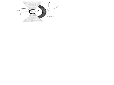
Figure 1: Example of CPLEAR event: like-strangeness $(K^{-},\Lambda)$

Fitting the decoherence parameter $\lambda$ by comparing the asymmetry (7.4) with the experimental data CPLEAR-EPR (see Fig.2) we find, when averaging over both configurations, the following bounds on $\lambda$

$$\bar{\lambda}\;=\;(1.84^{+2.50}_{-2.17})\cdot 10^{-12}\;\textrm{MeV}\quad\textrm{and}\quad\bar{\Lambda}\;=\;\frac{\bar{\lambda}}{\Gamma_{S}}\;=\;0.25^{+0.34}_{-0.32}\;.$$ (100)

The results (100) are certainly compatible with QM ($\lambda=0$), nevertheless, the experimental data allow an upper bound $\bar{\lambda}_{\textrm{up}}=4.34\cdot 10^{-12}\;\textrm{MeV}$ for possible decoherence in the entangled $K^{0}\bar{K}^{0}$ system.

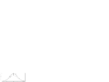
Figure 2: The asymmetry (7.4) as a function of the flight–path difference of the kaons. The dashed curve corresponds to QM, the solid curves represent the best fit (100) to the CPLEAR data CPLEAR-EPR , given by the crosses. The horizontal line indicates the Furry–Schrödinger’s hypothesis Schrodinger ; Furry , as explained in Sect. 8.

$B^{0}\bar{B}^{0}$ system: An analogous investigation of “decoherence of entangled beauty” has been carried out in Ref.BG3 . However, there time integrated events from the semileptonic decays of the entangled $B^{0}\bar{B}^{0}$ pairs are analyzed, which were produced at the colliders at DESY and Cornell. The analysis provides the bounds $\lambda_{B}=(-47\pm 76)\cdot 10^{-12}\;\textrm{MeV}$, which are an order of magnitude less restrictive than the bounds (100) of the $K^{0}\bar{K}^{0}$ system.

The possibility to measure the asymmetry at different times is offered now also in the $B$–meson system. Entangled $B^{0}\bar{B}^{0}$ pairs are created with high density at the asymmetric $B$–factories and identified by the detectors BELLE at KEK-B (see e.g. Refs. Belle ; Leder ) and BABAR at PEP-II (see e.g. Refs. Aubert ; Babar ) with a high resolution at different distances or times.

8 Connection to phenomenological model

There exists a simple procedure BG1 ; Dass ; BG2 for introducing decoherence in a rather phenomenological way, more in the spirit of Furry Furry and Schrödinger Schrodinger to describe the process of spontaneous factorization of the wavefunction. QM is modified in the sense that we multiply the interference term of the transition amplitude by the factor $(1-\zeta)$. The quantity $\zeta$ is called effective decoherence parameter. Starting again from the Bell singlet state $|\psi^{-}\rangle$, which is given by the mass eigenstate representation (90), we have for the like–strangeness probability

$$P(K^{0},t_{l};K^{0},t_{r})\;=\;||\langle K^{0}|_{l}\otimes\langle K^{0}|_{r}\;|\psi^{-}(t_{l},t_{r})\rangle||^{2}$$ (101)

$$\longrightarrow \quad P_{\zeta}(K^{0},t_{l};K^{0},t_{r})\;=\;\frac{1}{2}\;\biggl{\{}e^{-\Gamma_{S}t_{l}-\Gamma_{L}t_{r}}|\langle K^{0}|K_{S}\rangle_{l}|^{2}\;|\langle K^{0}|K_{L}\rangle_{r}|^{2}$$

$$+\;e^{-\Gamma_{L}t_{l}-\Gamma_{S}t_{r}}|\langle K^{0}|K_{L}\rangle_{l}|^{2}\;|\langle K^{0}|K_{S}\rangle_{r}|^{2}\;-\;2\;\underbrace{(1-\zeta)}\;e^{-\Gamma(t_{l}+t_{r})}$$

modification

$$\times\;\mathrm{Re}\big{\{}\langle K^{0}|K_{S}\rangle_{l}^{*}\langle K^{0}|K_{L}\rangle_{r}^{*}\langle K^{0}|K_{L}\rangle_{l}\langle K^{0}|K_{S}\rangle_{r}\;e^{-i\Delta m\Delta t}\big{\}}\biggr{\}}$$

$$= \frac{1}{8}\,\biggl{\{}e^{-\Gamma_{S}t_{l}-\Gamma_{L}t_{r}}+e^{-\Gamma_{L}t_{l}-\Gamma_{S}t_{r}}\;-\;2\,\underbrace{(1-\zeta)}\,e^{-\Gamma(t_{l}+t_{r})}\,\cos(\Delta m\Delta t)\biggr{\}}\,,$$

modification

and the unlike-strangeness probability just changes the sign of the interference term.

Features: The value $\zeta=0$ corresponds to pure QM and $\zeta=1$ to total decoherence or spontaneous factorization of the wave function, which is commonly known as Furry–Schrödinger hypothesis Schrodinger ; Furry . The decoherence parameter $\zeta$, introduced in this way “by hand”, is quite effective BG1 ; Dass ; BG2 ; BGH ; it interpolates continuously between the two limits: QM $\longleftrightarrow$ spontaneous factorization. It represents a measure for the amount of decoherence which results in a loss of entanglement of the total quantum state (we come back to this point in Section 9).

There exists a remarkable one–to–one correspondence between the model of decoherence (84), (85) and the phenomenological model, thus a relation between $\lambda\longleftrightarrow\zeta$ (Refs.BG3 ; BertlmannDurstbergerHiesmayr2002 ). We can see it quickly in the following way.

Calculating the asymmetry of strangeness events, as defined in Eq.(7.4), with the probabilities (101) we obtain

$$A^{\zeta}(t_{l},t_{r})\;=\;A^{QM}(\Delta t)\;\big{(}\,1\,-\,\zeta(t_{l},t_{r})\,\big{)}\;.$$ (102)

When we compare now the two approaches, i.e. Eq.(7.4) with Eq.(102), we find the formula

$$\zeta(t_{l},t_{r})\;=\;1\,-\;e^{-\lambda\min{\{t_{l},t_{r}\}}}\;.$$ (103)

Of course, when fitting the experimental data with the two models, the $\lambda$ values (100) are in agreement with the corresponding $\zeta$ values (averaged over both experimental setups) BGH ; trixi ,

$$\bar{\zeta}\;=\;0.13^{+0.16}_{-0.15}\;.$$ (104)

The phenomenological model demonstrates that the $K^{0}\bar{K}^{0}$ system is close to QM, i.e. $\zeta=0$, and (at the same time) far away from total decoherence, i.e. $\zeta=1$. It confirms nicely in a quantitative way the existence of entangled massive particles over macroscopic distances ($9$) cm.

We consider the decoherence parameter $\lambda$ to be the fundamental constant, whereas the value of the effective decoherence parameter $\zeta$ depends on the time when a measurement is performed. In the time evolution of the state $|\psi^{-}\rangle$, Eq.(90), represented by the density matrix (93), we have the relation

$$\zeta(t)\;=\;1\,-\;e^{-\lambda t}\;,$$ (105)

which after measurement of the left– and right–moving particles at $t_{l}$ and $t_{r}$ turns into formula (103), if decoherence occurs as described in Sect. 7.4.

Our model of decoherence has a very specific time evolution (103). Measuring the strangeness content of the entangled kaons at definite times we have the possibility to distinguish experimentally, on the basis of time dependent event rates, between the prediction of our model (103) and the results of other models (which would differ from Eq.(103)). Indeed, it is of high interest to measure in future experiments the asymmetry of the strangeness events at various times, in order to confirm the very specific time dependence of the decoherence effect. In fact, such a possibility is now offered in the $B$–meson system; as we already mentioned entangled $B^{0}\bar{B}^{0}$ pairs are created with high density at the asymmetric $B$–factories at KEK-B and at PEP-II.

9 Entanglement loss — decoherence

In the master equation (84) the dissipator $D[\rho]$ describes two phenomena occurring in an open quantum system, namely decoherence and dissipation (see, e.g., Ref. BreuerPetruccione ). When the system $S$ interacts with the environment $E$ the initially product state evolves into entangled states of $S+E$ in the course of time Joos ; KublerZeh . It leads to mixed states in $S$ —which means decoherence— and to an energy exchange between $S$ and $E$ —which is called dissipation.

The decoherence destroys the occurrence of long–range quantum correlations by suppressing the off-diagonal elements of the density matrix in a given basis and leads to an information transfer from the system $S$ to the
environment $E$:                   S$\rightleftarrows$      E

In general, both effects are present, however, decoherence acts on a much shorter time scale Joos ; JoosZeh ; Zurek ; Alicki than dissipation and is the more important effect in quantum information processes.

Our model describes decoherence and not dissipation. The increase of decoherence of the initially totally entangled $K^{0}\bar{K}^{0}$ system as time evolves means on the other hand a decrease of entanglement of the system. This loss of entanglement can be measured explicitly BertlmannDurstbergerHiesmayr2002 ; PHDtrixi .

In the field of quantum information the entanglement of a state is quantified by introducing certain entanglement measures. In this connection the entropy plays a fundamental role.

Entropy of a quantum system:

• The entropy measures the degree of uncertainty —the lack of knowledge— of a quantum state !

In general, a quantum state can be in a pure or mixed state (see, our discussion in Sect. 7.1). Whereas the pure state supplies us with maximal information about the system, a mixed state does not.

Proposition:  Thirring Thirring

• Mixed states provide only partial information about the system; the entropy measures how much of the maximal information is missing !

For mixed states the entanglement measures cannot be defined uniquely. Common measures of entanglement are von Neumann’s entropy function $S$, the entanglement of formation $E$ and the concurrence $C$.

9.1 Von Neumann entropy

We are only interested in the effect of decoherence, thus we properly normalize the state (93) in order to compensate for the decay property

$$\rho_{N}(t) = \frac{\rho(t)}{\mathrm{Tr}\rho(t)}\;.$$ (106)

Von Neumann’s entropy for the quantum state (106) is defined by

$$S\big{(}\rho_{N}(t)\big{)}\; = \;-\;\mathrm{Tr}\{\rho_{N}(t)\log_{2}\rho_{N}(t)\}$$

$$= \;-\frac{1-e^{-\lambda t}}{2}\log_{2}\frac{1-e^{-\lambda t}}{2}\;-\;\frac{1+e^{-\lambda t}}{2}\log_{2}\frac{1+e^{-\lambda t}}{2}\;,\hskip 14.22636pt$$ (107)

where we have chosen the logarithm to base $2$, the dimension of the Hilbert space (the qubit space), such that $S$ varies between $0\leq S\leq 1\,$.

Features:

1. $S\big{(}\rho_{N}(t)\big{)}=0$ for $t=0\,$; the entropy is zero at time $t=0\,$, there is no uncertainty in the system, the quantum state is pure and maximally entangled.

2. $S\big{(}\rho_{N}(t)\big{)}=1$ for $t\to\infty$; the entropy increases for increasing $t$ and approaches the value $1$ at infinity. Hence the state becomes more and more mixed.
   

Reduced density matrices:   Let us consider quite generally a composite quantum system $A$ (Alice) and $B$ (Bob). Then the reduced density matrix of subsystem $A$ is given by tracing the density matrix of the joint state over all states of $B$.

In our case the subsystems are the propagating kaons on the left $l$ and right $r$ hand side thus we have as reduced density matrices

$$\rho^{\,l}_{N}(t)=\mathrm{Tr}_{r}\{\rho_{N}(t)\}\quad\textrm{and}\quad\rho^{\,r}_{N}(t)=\mathrm{Tr}_{l}\{\rho_{N}(t)\}\;.$$ (108)

The uncertainty in the subsystem $l$ before the subsystem $r$ is measured is given by the von Neumann entropy $S(\rho^{\,l}_{N}(t))$ of the corresponding reduced density matrix $\rho^{\,l}_{N}(t)$ (and alternatively we can replace $l\to r$). In our case we find

$$S\big{(}\rho^{\,l}_{N}(t)\big{)}=S\big{(}\rho^{\,r}_{N}(t)\big{)}=1\;\qquad\forall\;t\geq 0\;.$$ (109)

The reduced entropies are independent of $\lambda$! That means the correlation stored in the composite system is, with increasing time, lost into the environment —what intuitively we had expected— and not into the subsystems, i.e. the individual kaons.

For pure quantum states von Neumann’s entropy function (9.1) is a good measure for entanglement and, generally, $A$ (Alice) and $B$ (Bob) are most entangled when their reduced density matrices are maximally mixed.

For mixed states, however, von Neumann’s entropy and the reduced entropies are no longer a good measure for entanglement so that we have to proceed in an other way to quantify entanglement (see Sect. 9.3).

9.2 Separability

In the following we want to show that the initially entangled Bell singlet state —although subjected to decoherence and thus to entanglement loss in the course of time— remains entangled. It is convenient to work with the “quasi–spin” description for the $K^{0}\bar{K}^{0}$ system (see Sect. 3). The projection operators of the mass eigenstates correspond to the spin projection operators “up” and “down”

$$P_{S} = |K_{S}\rangle\langle K_{S}|\;=\;\sigma_{\uparrow}\;=\;\frac{1}{2}\,(\mathbf{1}+\sigma_{z})\;=\;\left(\begin{array}[]{cc}1&0\\ 0&0\\ \end{array}\right)\;,$$ (112)

$$P_{L} = |K_{L}\rangle\langle K_{L}|\;=\;\sigma_{\downarrow}\;=\;\frac{1}{2}\,(\mathbf{1}-\sigma_{z})\;=\;\left(\begin{array}[]{cc}0&0\\ 0&1\\ \end{array}\right)\;,$$ (115)

and the transition operators are the “spin–ladder” operators

$$P_{SL} = |K_{S}\rangle\langle K_{L}|\;=\;\sigma_{+}\;=\;\frac{1}{2}\,(\sigma_{x}+i\,\sigma_{y})\;=\;\left(\begin{array}[]{cc}0&1\\ 0&0\\ \end{array}\right)\;,$$ (118)

$$P_{LS} = |K_{L}\rangle\langle K_{S}|\;=\;\sigma_{-}\;=\;\frac{1}{2}\,(\sigma_{x}-i\,\sigma_{y})\;=\;\left(\begin{array}[]{cc}0&0\\ 1&0\\ \end{array}\right)\;.$$ (121)

Then density matrix (106), (93) is expressed by the Pauli spin matrices in the following way

$$\rho_{N}(t)\,=\,\frac{1}{4}\big{\{}\mathbf{1}-\sigma_{z}\otimes\sigma_{z}\,-\,e^{-\lambda t}\,[\sigma_{x}\otimes\sigma_{x}+\sigma_{y}\otimes\sigma_{y}]\big{\}}\;,$$ (122)

which at $t=0$ coincides with the well-known expression for the pure spin singlet state $\rho_{N}(t=0)\,=\,\frac{1}{4}\,(\mathbf{1}-\vec{\sigma}\otimes\vec{\sigma})$; see, e.g., Ref. BNT .

Operator (122) can be nicely written as $4\times 4$ matrix

$$\rho_{N}(t)\;=\;\frac{1}{2}\left(\begin{array}[]{cccc}0&0&0&0\\ 0&1&-e^{-\lambda t}&0\\ 0&-e^{-\lambda t}&1&0\\ 0&0&0&0\\ \end{array}\right)\;.$$ (127)

For an other representation of the density matrix $\rho_{N}(t)$ we choose the so–called “Bell basis”

$$\rho^{\mp}\;=\;|\psi^{\mp}\rangle\langle\psi^{\mp}|\qquad\textrm{and}\qquad\omega^{\mp}\;=\;|\phi^{\mp}\rangle\langle\phi^{\mp}|\;,$$ (128)

with $|\psi^{-}\rangle$ given by Eq.(90) and $|\psi^{+}\rangle$ by

$$|\psi^{+}\rangle = \frac{1}{\sqrt{2}}\biggl{\{}|e_{1}\rangle+|e_{2}\rangle\biggr{\}}\;.$$ (129)

The states $|\phi^{\mp}\rangle=\frac{1}{\sqrt{2}}(|\Uparrow\Uparrow\rangle\mp|\Downarrow\Downarrow\rangle)$ (in spin notation) do not contribute here.

Entanglement — separability

Recall that in general the density matrix $\rho$ of a state is defined over the tensor product of Hilbert spaces $\mathcal{H}=\mathcal{H}_{A}\otimes\mathcal{H}_{B}$, named Alice and Bob.

A state $\rho$ is then called entangled if it is not separable, i.e. $\;\rho\in S^{c}$ where $S^{c}$ is the complement of the set of separable states $S$; and $S\cup S^{c}=\mathcal{H}$ .

Separable states:   The set of separable states is defined by

$$S\;=\;\Bigl{\{}\rho\,=\sum_{i}p_{i}\,\rho_{A}^{i}\otimes\rho_{B}^{i}\;\;\big{|}\;\;0\leq p_{i}\leq 1,\;\sum_{i}p_{i}=1\Bigr{\}}\;,$$ (130)

where $\rho_{A}^{i}$ and $\rho_{B}^{i}$ are density matrices over the subspaces $\mathcal{H}_{A}$ and $\mathcal{H}_{B}$.

The important question is now to judge whether a quantum state is entangled or conversely separable or not. Several separability criteria give an answer to that.

Theorem 9.1

Positive partial transpose criterion, Peres–Horodecki Peres ; Horodecki2
Defining the partial transposition $T_{B}$ by transposing only one of the subsystems, e.g. $T_{B}(\sigma^{i})_{kl}=(\sigma^{i})_{lk}\,$ in subsystem $B$, then a state $\rho$ is separable iff its partial transposition with respect to any subsystem is positive:

$$(\mathbbm{1}_{A}\otimes T_{B})\,\rho\,\geq\,0\quad\textrm{and}\quad(T_{A}\otimes\mathbbm{1}_{B})\,\rho\,\geq\,0\quad\;\Longleftrightarrow\quad\;\rho\;\;\mbox{separable}\;.$$ (131)

Theorem 9.2

Reduction criterion, Horodecki Horodecki
A state $\rho$ is separable for:

$$\mathbbm{1}_{A}\otimes\rho_{B}-\,\rho\,\geq\,0\quad\textrm{and}\quad\rho_{A}\otimes\mathbbm{1}_{B}-\,\rho\,\geq\,0\quad\;\Longleftrightarrow\quad\;\rho\;\;\mbox{separable}\;,$$ (132)

where $\rho_{A}$ is Alice’s reduced density matrix and $\rho_{B}$ Bob’s.

However, above Theorems (131), (132) are necessary and sufficient separability conditions —and so surprisingly simple— only for dimensions $2\otimes 2$ and $2\otimes 3$ HHHbook . A more general separability—entanglement criterion, valid in any dimensions, does exist; it is formulated by a so–called generalized Bell inequality, see Ref.BNT .

Now let us return to the question of entanglement and separability of our kaon quantum state described by density matrix $\rho_{N}(t)$ (106), (93) as it evolves in time.

Proposition:  Bertlmann–Durstberger–Hiesmayr BertlmannDurstbergerHiesmayr2002

• The state represented by the density matrix $\rho_{N}(t)$ (106), (93) becomes mixed for $0<t<\infty$ but remains entangled. Separability is achieved asymptotically $t\to\infty$ with the weight $e^{-\lambda t}$. Explicitly, $\rho_{N}(t)$ is the following mixture of the Bell states $\rho^{-}$ and $\rho^{+}\,$:

  $$\rho_{N}(t)\;=\;\frac{1}{2}\big{(}1+e^{-\lambda t}\big{)}\,\rho^{-}\;+\;\frac{1}{2}\big{(}1-e^{-\lambda t}\big{)}\,\rho^{+}\;.\\$$ (133)

Proof:

• The mixedness of the state, with $t\to\infty$ totally mixed — separable, can be seen from the mixed state criterion (see Sect. 7.1)

  $$\rho^{\,2}_{N}(t)\;=\;\frac{1}{4}\left(\begin{array}[]{cccc}0&0&0&0\\ 0&1+e^{-2\lambda t}&-2e^{-\lambda t}&0\\ 0&-2e^{-\lambda t}&1+e^{-2\lambda t}&0\\ 0&0&0&0\\ \end{array}\right)\;\not=\;\rho_{N}(t)\quad\textrm{for}\quad t>0\;.$$ (138)

• Entanglement or lack of separability is determined by Theorems (131) and (132). The Peres–Horodecki partial transposition criterion (131)

  $$(\mathbf{1}_{l}\otimes T_{r})\,\rho_{N}(t)\; = \;\frac{1}{2}\left(\begin{array}[]{clrc}0&0&0&-e^{-\lambda t}\\ 0&1&0&0\\ 0&0&1&0\\ -e^{-\lambda t}&0&0&0\\ \end{array}\right)\not\geq 0\;,$$ (143)

  with eigenvalues $\big{\{}\frac{1}{2},\frac{1}{2},\frac{1}{2}e^{-\lambda t},-\frac{1}{2}e^{-\lambda t}\big{\}}\;$, is not positive. Alternatively, the Horodecki reduction criterion (132), a matrix with same eigenvalues (143)

  $$\mathbf{1}_{l}\otimes\rho^{\,r}_{N}(t)-\rho_{N}(t)\;=\;\frac{1}{2}\left(\begin{array}[]{cccc}1&0&0&0\\ 0&0&e^{-\lambda t}&0\\ 0&e^{-\lambda t}&0&0\\ 0&0&0&1\\ \end{array}\right)\not\geq 0\;,$$ (148)

  is not positive either. Therefore $\rho_{N}(t)$ remains entangled for $t<\infty$. $\Box$

9.3 Entanglement of formation and concurrence

For pure states the entropy of the reduced density matrices is sufficient, for mixed states we need another measure, e.g., entanglement of formation.

Entanglement of formation

Every density matrix $\rho$ can be decomposed into an ensemble of pure states $\rho_{i}=|\psi_{i}\rangle\langle\psi_{i}|$ with the probability $p_{i}$, i.e. $\rho=\sum_{i}p_{i}\rho_{i}$. The entanglement of formation for a pure state is given by the entropy of either of the two subsystems. For a mixed state entanglement of formation Bennett-entangle is defined as average entanglement of pure states of the decomposition, minimized over all decompositions of $\rho$

$$E(\rho) = \min\sum_{i}\,p_{i}\,S(\rho_{i}^{\,l})\;.$$ (149)

It quantifies the resources needed to create a given entangled state. Bennett et al. Bennett-entangle found a remarkable simple formula for entanglement of formation

$$E(\rho) \geq \mathcal{E}\big{(}f(\rho)\big{)}\;,$$ (150)

where the function $\mathcal{E}\big{(}f(\rho)\big{)}$ is defined by

$$\mathcal{E}\big{(}f\big{)}\;=\;H\bigg{(}\frac{1}{2}+\sqrt{f(1-f)}\bigg{)}\quad\textrm{for}\quad f\geq\frac{1}{2}\;,$$ (151)

and $\mathcal{E}\big{(}f\big{)}=0$ for $f<\frac{1}{2}\,$. The function $H$ represents the familiar binary entropy function $H(x)=-x\log_{2}x-(1-x)\log_{2}(1-x)$. The quantity $f(\rho)$ is called the fully entangled fraction of $\rho$

$$f(\rho)=\max\,\langle e|\rho|e\rangle\;,$$ (152)

which is the maximum over all completely entangled states $|e\rangle$.

For general mixed states $\rho$ the function $\mathcal{E}\big{(}f(\rho)\big{)}$ is only a lower bound to the entropy $E(\rho)$. For pure states and mixtures of Bell states —the case of our model— the bound is saturated, $E=\mathcal{E}$, and we have formula (151) for calculating the entanglement of formation.

Concurrence

Wootters and Hill Wootters1 ; Wootters2 ; Wootters3 found that entanglement of formation for a general mixed state $\rho$ of two qubits can be expressed by another quantity, the concurrence $C$

$$E(\rho)\; = \;\mathcal{E}\big{(}C(\rho)\big{)}\;=\;H\bigg{(}\frac{1}{2}+\frac{1}{2}\sqrt{1-C^{2}}\bigg{)}\quad\textrm{with}\quad 0\leq C\leq 1\;.$$ (153)

Explicitly, the function $\mathcal{E}(C)$ looks like

$$\mathcal{E}(C) = -\frac{1+\sqrt{1-C^{2}}}{2}\log_{2}\frac{1+\sqrt{1-C^{2}}}{2}-\frac{1-\sqrt{1-C^{2}}}{2}\log_{2}\frac{1-\sqrt{1-C^{2}}}{2}$$

and is monotonically increasing from $0$ to $1$ as $C$ runs from $0$ to $1$. Thus $C$ itself is a kind of entanglement measure in its own right.

Defining the spin flipped state $\tilde{\rho}$ of $\rho$ by

$$\tilde{\rho}\; = \;(\sigma_{y}\otimes\sigma_{y})\,\rho^{*}(\sigma_{y}\otimes\sigma_{y})\;,$$ (155)

where $\rho^{*}$ is the complex conjugate and is taken in the standard basis, i.e. the basis $\{|\Uparrow\Uparrow\rangle,|\Downarrow\Downarrow\rangle,|\Uparrow\Downarrow\rangle,|\Downarrow\Uparrow\rangle\}$, the concurrence $C$ is given by the formula

$$C(\rho)\; = \;\max\{0,\lambda_{1}-\lambda_{2}-\lambda_{3}-\lambda_{4}\}\;.$$ (156)

The $\lambda_{i}$’s are the square roots of the eigenvalues, in decreasing order, of the matrix $\rho\tilde{\rho}$.

Applications to our model

For the density matrix $\rho_{N}(t)$ (106) of our model, which is invariant under spin flip, i.e. $\tilde{\rho}_{N}=\rho_{N}$ and thus $\rho_{N}\tilde{\rho}_{N}=\rho^{\,2}_{N}$, we obtain for the concurrence

$$C\big{(}\rho_{N}(t)\big{)}\; = \;\max\big{\{}0,e^{-\lambda t}\big{\}}\;=\;e^{-\lambda t}\;,$$ (157)

and for the fully entangled fraction of $\rho_{N}(t)$

$$f\big{(}\rho_{N}(t)\big{)}\;=\;\frac{1}{2}\big{(}1+e^{-\lambda t}\big{)}\;,$$ (158)

which is simply the largest eigenvalue of $\rho_{N}(t)$. Clearly, in our case the functions $C$ and $f$ are related by

$$C\big{(}\rho_{N}(t)\big{)}\; = \;2\,f\big{(}\rho_{N}(t)\big{)}-1\;.$$ (159)

Finally, we have for the entanglement of formation of the $K^{0}\bar{K}^{0}$ system

$$E\big{(}\rho_{N}(t)\big{)}\; = \;-\frac{1+\sqrt{1-e^{-2\lambda t}}}{2}\log_{2}\frac{1+\sqrt{1-e^{-2\lambda t}}}{2}$$ (160)

$$-\frac{1-\sqrt{1-e^{-2\lambda t}}}{2}\log_{2}\frac{1-\sqrt{1-e^{-2\lambda t}}}{2}\;.$$

Using now our relation (105) between the decoherence parameters $\lambda$ and $\zeta$ we find a striking connection between the entanglement measure, defined by the entropy of the state, and the decoherence of the quantum system, which describes the amount of factorization into product states (Furry–Schrödinger hypothesis Schrodinger ; Furry ).

Loss of entanglement: Defining the loss of entanglement as the gap between an entanglement value and its maximum unity, we find

$$1-C\big{(}\rho_{N}(t)\big{)}\; = \;\zeta(t)\;,$$ (161)

$$1-E\big{(}\rho_{N}(t)\big{)}\; \doteq \;\frac{1}{\ln 2}\;\zeta(t)\;\doteq\;\frac{\lambda}{\ln 2}\;t\;,$$ (162)

where in Eq.(162) we have expanded expression (160) for small values of the parameters $\lambda$ or $\zeta$.

We get the following proposition.

Proposition:  Bertlmann–Durstberger–Hiesmayr BertlmannDurstbergerHiesmayr2002

• The entanglement loss equals the decoherence !
  

Therefore we are able to determine experimentally the degree of entanglement of the $K^{0}\bar{K}^{0}$ system, namely by considering the asymmetry (7.4) and fitting the parameter $\zeta$ or $\lambda$ to the data.

Results

In Fig.3 we have plotted the loss of entanglement $1-E$, given by Eq.(160), as compared to the loss of information, the von Neumann entropy function $S$, Eq.(9.1), in dependence of the time $t/\tau_{s}$ of the propagating $K^{0}\bar{K}^{0}$ system. The loss of entanglement of formation increases slower with time and visualizes the resources needed to create a given entangled state. At $t=0$ the pure Bell state $\rho^{-}$ is created and becomes mixed for $t>0$ by the other Bell state $\rho^{+}$. In the total state the amount of entanglement decreases until separability is achieved (exponentially fast) for $t\to\infty$.

In case of the CPLEAR experiment, where one kaon propagates about $2$ cm, corresponding to a propagation time $t_{0}/\tau_{s}\approx 0.55$, until it is measured by an absorber, the entanglement loss is about $18\%$ for the mean value and maximal $38\%$ for the upper bound of the decoherence parameter $\lambda$.

Figure 3: The time dependence of the von Neumann entropy (dashed lines), Eq.(9.1), and the loss of entanglement of formation $1-E$ (solid lines), given by Eq.(160), are plotted for the experimental mean value $\bar{\lambda}=1.84\cdot 10^{-12}\;\textrm{MeV}$ (lower curve) and the upper bound $\bar{\lambda}_{up}=4.34\cdot 10^{-12}\;\textrm{MeV}$ (upper curve), Eq.(100), of the decoherence parameter $\lambda$. The time $t$ is scaled versus the lifetime $\tau_{s}$ of the short–lived kaon $K_{S}$: $t\to t/\tau_{s}$. The vertical lines represent the propagation time $t_{0}/\tau_{s}\approx 0.55$ of one kaon, including the experimental error bars, until it is measured by the absorber in the CPLEAR experiment.

10 Outlook

Entanglement is the basic ingredient for quantum communication and computation, its effects will become important for future technologies. The fast developments in quantum information stimulated research in particle physics, which may have effects we cannot foresee now. We are sure that in future there will be a fruitful exchange between particle physics and quantum optics.

There are close analogies but also significant differences between entangled meson–antimeson systems and entangled photon or spin–$\frac{1}{2}$ systems. It turns out that quantum mechanical tests of meson–antimeson systems are more subtle than those of photon systems and one has to take into account the features of the mesons, which are characteristic for such massive quantum systems. It is the decay property or a symmetry violation property, like $CP$ violation, or the regeneration property of the quantum state.

Bell inequalities

Generally, Bell inequalities for meson–antimeson systems contain both the freedom of choice in time and in quasi–spin (see Sect. 6.2). As we concluded in Sect. 6.3 the time variation type of BI, however, cannot be used to exclude LRT for the familiar meson–antimeson systems due to the (unfortunate) interplay between flavor oscillation (e.g., strangeness, beauty, charm, …) and decay time BertlmannHiesmayr2001 ; ghirardi91 ; ghirardi92 ; trixi .

In this connection we would like to mention that the work of Ref.Go , analyzing entangled $B^{0}\bar{B}^{0}$ meson pairs produced at the KEKB asymmetric $e^{+}e^{-}$ collider and collected at the BELLE detector, is hardly relevant for the test of QM versus LRT. The reasons are twofold: Firstly, “active” measurements are missing, therefore one can construct a local realistic model; secondly, the unitary time evolution of the unstable quantum state —the decay property of the meson— is ignored, which is part of its nature (for more detailed criticism, see Ref.BertlmannHiesmayrBramonGarbarino ). Nevertheless, the work Go represents a notable test of QM correlations exhibited by $B^{0}\bar{B}^{0}$ entangled pairs and further investigations along these lines are recommended.

Considering, on the other hand, a BI at fixed time but for quasi–spin variation, a Wigner–like BI for the several types of the K–meson (see Sect. 6.4), provides an inequality for a symmetry violation parameter, the physical $CP$ violation parameter (charge conjugation and parity) in our case Uchiyama ; BGH-CP . Experimentally it is tested by studying the leptonic charge asymmetry $\delta$ of the $K_{L}$ type. It is remarkable that the premises of LRT are only compatible with strict $CP$ conservation, i.e. with $\delta=0$. In this way, $\delta\neq 0$ is a manifestation of the entanglement of the considered state. We have found the following proposition.

Proposition:  Bertlmann–Grimus–Hiesmayr BGH-CP

• $CP$ violation in $K^{0}\bar{K}^{0}$ mixing leads to violation of a BI !

We do believe that this connection between symmetry violation and BI violation is part of a more general quantum feature, therefore studies of other particle symmetries in this connection would be of high interest.

Bramon et al. Bramon ; AncoBramon ; BramonGarbarino have established novel BI’s for entangled $K^{0}\bar{K}^{0}$ pairs by using the well–known regeneration mechanism of the kaons (see Sect. 2.4). After producing kaon pairs at the $\Phi$ resonance a thin regenerator (with kaon crossing time $t_{\textrm{cross}}\ll\tau_{S}$) is placed into one kaon beam near the $\Phi$ decay point. Then the entangled state contains a term proportional to $r\,|K_{L}\rangle_{l}\otimes|K_{L}\rangle_{r}$, where $r$ denotes the regeneration parameter, a well–defined quantity being proportional to the difference of the $K^{0}N$ and $\bar{K}^{0}N$ amplitudes. Allowing the entangled state to propagate up to a time $T$, with $\tau_{S}\ll T\ll\tau_{L}$, in each beam of the two sides either the lifetime/decay states $K_{S}$ versus $K_{L}$ or the strangeness states $K^{0}$ versus $\bar{K}^{0}$ are measured. Considering Clauser–Horne–type inequalities ClauserHorne a set of inequalities for the parameter $R=-r\,\exp{[-i\Delta m+\frac{1}{2}(\Gamma_{S}-\Gamma_{L})]\,T}$ can be derived. One of the inequalities is —under certain conditions (for the regeneration, etc…)— violated by QM. It provides an interesting experimental test at $\Phi$–factories or $p\bar{p}$ machines in the future.

Decoherence

We have developed a general but quite simple and practicable procedure to estimate quantitatively the degree of possible decoherence of a quantum state due to some interaction of the state with its “environment” (see Sect. 7). This is of special interest in case of entangled states where a single parameter, the decoherence parameter $\lambda$ or $\zeta$ BG3 ; BertlmannDurstbergerHiesmayr2002 ; BGH , quantifies the strength of decoherence between the two subsystems or the amount of spontaneous factorization of the wavefunction. The asymmetry of like– and unlike–flavor events is directly sensitive to $\lambda$ or $\zeta$.

On the other hand, we have found a bridge to common entanglement measures, such as entanglement of formation and concurrence (see Sect. 9), and could derive the Proposition that the entanglement loss equals the decoherence ! In this way we also measure the amount of entanglement of the state.

Using experimental data of the CPLEAR experiment provides us with upper bounds to the decoherence and the entanglement loss of the $K^{0}\bar{K}^{0}$ state produced in $p\bar{p}$ collisions, which is of macroscopic extent ($9$ cm).

As up to now only two data points are available, further experimental data are certainly highly desirable and would sharpen the bounds considerably. Such data could be collected at the $\Phi$–factory DA$\Phi$NE in Frascati. In this connection, a recent analysis of entangled $K_{S}K_{L}$ systems by the KLOE collaboration KLOE-Domenico sets new bounds on the decoherence parameter $\zeta$.

Indeed, it would be of great interest to measure in future experiments the asymmetry of like– and unlike–flavor events for several different times, in order to confirm the time dependence of the decoherence effect. In fact, such a possibility is now offered in the $B$-meson system. As already mentioned (Sect. 7.4) entangled $B^{0}\bar{B}^{0}$ pairs are created with high density at the asymmetric $B$-factories and identified by the detectors BELLE at KEK-B Belle ; Leder and BABAR at PEP-II Aubert ; Babar with a high resolution at different distances or times. On the basis of the time dependent event rates we could test experimentally the predictions of our decoherence model.

Of course, these decoherence investigations could be performed with other entangled systems, like photonic systems, as well.

Complementarity

Meson systems in particle physics are also an interesting testing ground for basic principles of QM such as quantitative wave–particle duality SBGH3 ; SBGH4 or quantum marking and quantum erasure SBGH1 ; SBGH2 .

Bohr’s complementarity principle (or duality principle) can be formulated in a quantitative way GreenbergerYasin ; Englert by defining on one hand the fringe visibility —the sharpness of the interference pattern, the wave–like property— and on the other the path predictability, e.g., in a two–path interferometer RauchWerner . This “which–way” knowledge on the path taken by the interfering system expresses the particle–like property of the system.

Considering now a produced $K^{0}$ beam, it oscillates between $K^{0}$ and $\bar{K}^{0}$ but it also represents a superposition of $K_{S}$ and $K_{L}$ which decay at totally different rates (recall Sect. 2). Then the strangeness oscillations can be viewed as fringe visibility and the $K_{S}$ and $K_{L}$ states with their different decay distances as the analogues of the two paths in the interferometer. The comparison of present data with the calculations of this kind of kaon interferometry satisfies nicely the statement of quantitative duality SBGH3 ; SBGH4 . Further experiments, e.g., at the $\Phi$–factory DA$\Phi$NE are of interest in this connection.

Geometric phase — entanglement

An interesting question is: how can we influence the entanglement of a spin–$\frac{1}{2}$ system by creating a geometric phase? Geometric phases such as the Berry phase Berry1 play a considerable role in physics and arise in a quantum system when its time evolution is cyclic and adiabatic. There is increasing interest in combining both the geometric phase and the entanglement of a system Sjoqvist2000 ; TongKwekOh2003 ; MilmanMosseri2003 ; TongSjoqvistKwekOhEricsson ; BDHH .

In Ref.BDHH we have studied the influence of the Berry phase on the entanglement of a spin–$\frac{1}{2}$ system by generating the Berry phase with an adiabatically rotating magnetic field in one of the paths of the particles, and we have eliminated the dynamical phase —being sensitive just to the geometric phase— by a “spin–echo” method. We have considered a pure entangled system where a phase —like our geometrical one— does not change the amount of entanglement and therefore not the extent of nonlocality of the system, which is determined by the maximal violation of a BI. In our case the Berry phase just affects the Bell angles in a specific way. On the other hand, keeping the measurement planes fixed the polar Bell angles vary and the maximum of the $S$-function of the CHSH inequality (recall Sect. 5) varies with respect to the Berry phase.

We have applied the investigation to neutron interferometry where one can achieve entanglement between different degrees of freedom —an internal and external one— the spin and the path of the neutron. In this case it is physically rather contextuality than nonlocality which is tested experimentally BDHH ; RauchWerner ; BasuBandyopadhyayKarHome ; HasegawaLoidlBadurekBaronRauch .

There are still open problems in how does entanglement behave —the several entanglement measures— if geometric phases are introduced into mixed quantum states. How do they change entanglement? What happens to the Berry phase of the system if in addition we allow for interaction of the quantum system with an environment, thus allowing for decoherence? How can it be experimentally realized? Work along these lines is of increasing interest FonsecaAguiarThomaz ; KamleitnerCresserSanders ; Carollo-Vedral ; DoddHalliwell ; WhitneyGefen .

Generalized Bell inequality — entanglement witness

In quantum communication, the two remote parties, Alice and Bob, want to carry out a certain task with minimal communication. Comparing now the amount of communication necessary by using classical or quantum bits, it turns out that sharing entangled quantum states —instead of classical or separable ones— leads to savings in the communication. That makes entangled states so important in quantum communication technology.

But how do we witness an entangled state? Via the familiar Bell inequalities described before (Sect. 5)? Yes, if the states are pure entangled states but no if they are mixed entangled. Werner Werner found out that a certain mixture of entangled and separable states, so–called Werner states, do satisfy the familiar BI. Thus the importance of the BI is that they serve as criterion for nonlocality —as departures from LRT— and they are valuable when considering phenomena like quantum teleportation or quantum cryptography. But as a criterion for separability they are rather poor.

There exist, however, some operators, so–called entanglement witnesses, satisfying an inequality, a generalized Bell inequality (GBI), for all separable states and violating this inequality for an entangled state BNT ; HHH96 ; TerhalPhysLett ; Bruss .

In Ref.BNT we have studied the class of entanglement witnesses; considering density matrices (states) and operators (entanglement witnesses) as elements of a Hilbert space it turns out that entanglement witnesses are tangent functionals to the set of separable states. Considering the Euclidean distance of the vectors in Hilbert space for entangled and separable states we have found the following Theorem.

Theorem:  Bertlmann–Narnhofer–Thirring BNT

• The Euclidean distance of an entangled state to the separable states is equal to the maximal violation of the GBI with the tangent functional as entanglement witness !
  

Viewing the Euclidean distance as entanglement measure we have found a nice geometric picture for entanglement (and its value), for GBI (and its maximal violation) and for the tangent functional which characterizes (as a tangent) the set of separable states. All three conceptions are only different aspects of the same geometric picture. It is especially illustrative for the example of two spins, Alice and Bob. In this connection investigations for multi–particle entangled states, e.g., GHZ–states GHZ ; GHZ-Shimony , are certainly of high interest.

11 Acknowledgement

The author wants to take the opportunity to thank his collaborators and friends for all the joyful discussions about this field, special thanks go to Markus Arndt, Katharina Durstberger, Gerhard Ecker, Stefan Filipp, Walter Grimus, Yuji Hasegawa, Beatrix Hiesmayr, Heide Narnhofer, Helmut Neufeld, Herbert Pietschmann, Helmut Rauch, Walter Thirring and Anton Zeilinger. The aid of EU project EURIDICE EEC-TMR program HPRN-CT-2002-00311 is acknowledged. Finally, I would like to thank the organizers of the Schladming School for creating such a stimulating scientific atmosphere.

References

- (1) E. Schrödinger: Naturwissenschaften 23, 807 (1935); 23, 823 (1935); 23, 844 (1935)
- (2) A. Einstein, B. Podolski, N. Rosen: Phys. Rev. 47, 777 (1935)
- (3) N. Bohr: Phys.Rev. 48, 696 (1935)
- (4) W.H. Furry: Phys. Rev. 49, 393 (1936); ibid. 49, 476 (1936)
- (5) J.S. Bell: Physics 1, 195 (1964)
- (6) R.A. Bertlmann: Found. Phys. 20, 1191 (1990)
- (7) S.J. Freedman, J.F. Clauser: Phys. Rev. Lett. 28, 938 (1972)
- (8) E.S. Fry, R.C. Thompson: Phys. Rev. Lett. 37, 465 (1976)
- (9) A. Aspect, P. Grangier, G. Roger: Phys. Rev. Lett. 49, 91 (1982); A. Aspect, J. Dalibard, G. Roger: Phys. Rev. Lett. 49, 1804 (1982)
- (10) G. Weihs, T. Jennewein, C. Simon, H. Weinfurter, A. Zeilinger: Phys. Rev. Lett. 81, 5039 (1998)
- (11) W. Tittel, G. Ribordy, N. Gisin: Physics World 11, No.3, p.41 (1998); W. Tittel, J. Brendel, H. Zbinden, N. Gisin: Phys. Rev. Lett. 81, 3563 (1998); H. Zbinden, J. Brendel, W. Tittel, N. Gisin: Phys. Rev. A 63, 022111 (2001)
- (12) M. Aspelmeyer, H.R. Böhm, T. Gyatso, T. Jennewein, R. Kaltenbaek, M. Lindenthal, G. Molina-Terriza, A. Poppe, K. Resch, M. Taraba, R. Ursin, P. Walther, A. Zeilinger: Science 301, 621 (2003)
- (13) J.S. Bell: Speakable and Unspeakable in Quantum Mechanics (Cambridge University Press 1987)
- (14) A.K. Ekert: Phys. Rev. Lett. 67, 661 (1991)
- (15) D. Deutsch, A.K. Ekert: Physics World 11, No.3, p.47 (1998)
- (16) R.J. Hughes: Contemp. Phys. 36, 149 (1995)
- (17) C.H. Bennett, G. Brassard, C. Crépeau, R. Jozsa, A. Peres, W.K. Wootters: Phys. Rev. Lett. 70, 1895 (1993)
- (18) J.-W. Pan, D. Bouwmeester, H. Weinfurter, A. Zeilinger: Nature 390, 575 (1997)
- (19) A. Zeilinger: Physics World 11, No.3, 35 (1998)
- (20) D. Bouwmeester, A. Ekert, A. Zeilinger: The physics of quantum information: quantum cryptography, quantum teleportation, quantum computations (Springer, Berlin Heidelberg New York 2000)
- (21) R. A. Bertlmann, A. Zeilinger (eds.): Quantum [Un]speakables, from Bell to Quantum Information (Springer, Berlin Heidelberg New York 2002)
- (22) T.D. Lee, C.N. Yang: reported by T.D. Lee at Argonne National Laboratory, May 28, 1960 (unpublished)
- (23) D.R. Inglis: Rev. Mod. Phys. 33, 1 (1961)
- (24) T.B. Day: Phys. Rev. 121, 1204 (1961)
- (25) H.J. Lipkin: Phys. Rev. 176, 1715 (1968)
- (26) P.H. Eberhard: in The Second Dane Physics Handbook, edited by L. Maiani, G. Pancheri, N. Paver (SIS–Pubblicazioni dei Laboratori di Frascati, Italy, 1995) Vol I, p. 99
- (27) P.H. Eberhard: Nucl. Phys. B 398, 155 (1992)
- (28) I.I. Bigi: Nucl. Phys. B (Proc. Suppl.) 24A, 24 (1991)
- (29) A. Di Domenico: Nucl. Phys. B 450, 293 (1995)
- (30) A. Bramon, M Nowakowski: Phys. Rev. Lett. 83, 1 (1999)
- (31) B. Ancochea, A. Bramon, M Nowakowski: Phys. Rev. D 60, 094008 (1999)
- (32) A. Bramon, G. Garbarino: Phys. Rev. Lett. 88, 040403 (2002)
- (33) M. Genovese, C. Novero, E. Predazzi: Phys. Lett. B 513, 401 (2001)
- (34) J. Six: Phys. Lett. B 114, 200 (1982)
- (35) A. Apostolakis et al.: CPLEAR Coll., Phys. Lett. B 422, 339 (1998)
- (36) R.A. Bertlmann, W. Grimus, B.C. Hiesmayr: Phys. Rev. D 60, 114032 (1999)
- (37) R.A. Bertlmann, W. Grimus: Phys. Lett. B 392, 426 (1997)
- (38) G.V. Dass, K.V.L. Sarma: Eur. Phys. J. C 5, 283 (1998)
- (39) R.A. Bertlmann, W. Grimus: Phys. Rev. D 58, 034014 (1998)
- (40) A. Datta, D. Home: Phys. Lett. A 119, 3 (1986)
- (41) A. Pompili, F. Selleri: Eur. Phys. J. C 14, 469 (2000)
- (42) R.A. Bertlmann, W. Grimus: Phys. Rev. D 64, 056004 (2001)
- (43) F. Selleri: Lett. Nuovo Cim. 36, 521 (1983); P. Privitera, F. Selleri: Phys. Lett. B 296, 261 (1992); F. Selleri: Phys. Rev. A 56, 3493 (1997); R. Foadi, F. Selleri: Phys. Rev. A 61, 012106 (1999); R. Foadi, F. Selleri: Phys. Lett. B 461, 123 (1999)
- (44) A. Afriat, F. Selleri: The Einstein, Podolsky, and Rosen Paradox in Atomic, Nuclear and Particle Physics, (Plenum Press, New York London 1999)
- (45) J. Six: Phys. Lett. A 150, 243 (1990)
- (46) A. Bramon, G. Garbarino: Phys. Rev. Lett. 89, 160401 (2002)
- (47) R. A. Bertlmann, B. C. Hiesmayr: Phys. Rev. A 63, 062112 (2001)
- (48) R. A. Bertlmann, K. Durstberger, B. C. Hiesmayr: Phys. Rev. A 68, 012111 (2003)
- (49) M. Gell-Mann, A. Pais: Phys. Rev. 97, 1387 (1955)
- (50) A. Pais, O. Piccioni: Phys. Rev. 100, 1487 (1955)
- (51) J.S. Bell: Proceedings of the Royal Society A 231, 479 (1955)
- (52) W. Pauli: Niels Bohr and the development of physics, (McGraw-Hill, New York 1955); Nuovo Cimento 6, 204 (1957)
- (53) G. Lüders: Kgl. Danske Vidensk. Selsk. Mat.-Fys. Medd 28, no.5 (1954); Ann. Phys. 2, 1 (1957)
- (54) T.D. Lee, C.S. Wu: Ann. Rev. Nucl. Sci. 16, 511 (1966)
- (55) J.S. Bell, J. Steinberger: Weak Interactions of Kaons, Proceedings of the Oxford International Conference, 19-25 Sept., p. 147, (1965)
- (56) G.C. Ghirardi, R. Grassi, T. Weber: in Proc. of Workshop on Physics and Detectors for DANE, the Frascati Factory, April 9-12th, 1991, edited by G. Pancheri, p. 261
- (57) J.E. Clauser, M.A. Horne, A. Shimony, R.A. Holt: Phys. Rev. D 10, 880 (1969)
- (58) J.S. Bell: Introduction to the Hidden–Variable Question. Article 4 in Ref.bell2
- (59) J.E. Clauser, A. Shimony: Rep. Prog. Phys. Vol. 41, 1881 (1978)
- (60) E.P. Wigner: Am. J. Phys. 38, 1005 (1970)
- (61) N. Gisin, A. Go: Am. J. Phys. 69 (3), 264 (2001)
- (62) G.C. Ghirardi, R. Grassi, R. Ragazzon: in The DANE Physics Handbook, Vol. I, ed. by L. Maiani, G. Pancheri and N. Paver (Servizio Documentazione dei Laboratori Nazionale di Frascati, Italy 1992), p. 283
- (63) B.C. Hiesmayr: The puzzling story of the –system or about quantum mechanical interference and Bell inequalities in particle physics, Master Thesis, University of Vienna, (1999)
- (64) B.C. Hiesmayr: private communication
- (65) F. Uchiyama: Phys. Lett. A 231, 295 (1997)
- (66) D.E. Groom et al: Review of Particle Physics, Eur. Phys. J. C 3, 1 (1998)
- (67) R.A. Bertlmann, W. Grimus, B.C. Hiesmayr: Phys. Lett. A 289, 21 (2001)
- (68) J.S. Bell: Rev. Mod. Phys. 38, 447 (1966); S. Kochen, E.P. Specker: J. Math. Mech. 17, 59 (1967); N.D. Mermin: Rev. Mod. Phys. 65, 803 (1993)
- (69) S. Hawking: Commun. Math. Phys. 87, 395 (1982)
- (70) G. ‘t Hooft: Class. Quant. Grav. 16, 3263 (1999)
- (71) G. ‘t Hooft: Determinism and Dissipation in Quantum Gravity, hep-th/ 0003005 (2000)
- (72) G.C. Ghirardi, A. Rimini, and T. Weber: Phys. Rev. D 34, 470 (1986)
- (73) P. Pearle: Phys. Rev. A 39, 2277 (1989)
- (74) N. Gisin, I.C. Percival: J. Phys. A: Math. Gen. 25, 5677 (1992); ibid. 26, 2245 (1993)
- (75) R. Penrose: Gen. Rel. Grav. 28, 581 (1996); Phil. Trans. Roy. Soc. Lond. A 356, 1927 (1998)
- (76) G. Lindblad: Comm. Math. Phys. 48, 119 (1976)
- (77) V. Gorini, A. Kossakowski, E.C.G. Sudarshan: J. Math. Phys. 17, 821 (1976)
- (78) R.A. Bertlmann, W. Grimus: Phys. Lett. A 300, 107 (2002)
- (79) S.L. Adler: Phys. Rev. D 62, 117901 (2000)
- (80) F. Benatti, H. Narnhofer: Lett. Math. Phys. 15, 325 (1988)
- (81) BELLE-homepage: http://belle.kek.jp
- (82) G. Leder: talk given at the conference SUSY’02, Hamburg June 2002, http://wwwhephy.oeaw.ac.at/p3w/belle/leder_susy02.pdf (unpublished)
- (83) B.Aubert et al.: BABAR Collaboration, Phys. Rev. D. 66, 032003 (2002)
- (84) BABAR-homepage: http://www.slac.stanford.edu/babar
- (85) H.-P. Breuer, F. Petruccione: The theory of open quantum systems, (Oxford University Press 2002)
- (86) E. Joos: Decoherence through interaction with the environment, in: Decoherence and the apperance of a classical world in quantum theory, D. Giulini et al. (eds.) (Springer Verlag, Heidelberg, 1996) p.35
- (87) O. Kübler, H.D. Zeh: Ann. Phys. (N.Y.) 76, 405 (1973)
- (88) E. Joos, H.D. Zeh: Z. Phys. B 59, 223 (1985)
- (89) W.H. Zurek: Physics Today 44, 36 (1991)
- (90) R. Alicki: Phys. Rev. A 65, 034104 (2002)
- (91) B.C. Hiesmayr: The puzzling story of the neutral kaon system or what we can learn of entanglement, Ph.D. Thesis, University of Vienna, 2002
- (92) W. Thirring: Lehrbuch der Mathematischen Physik 4, Quantenmechanik großer Systeme (Springer Verlag, Wien 1980)
- (93) R.A. Bertlmann, H. Narnhofer, W. Thirring: Phys. Rev. A 66, 032319 (2002)
- (94) A. Peres: Phys. Rev. Lett. 77, 1413 (1996)
- (95) M. Horodecki, P. Horodecki, R. Horodecki: Phys. Lett. A 223, 1 (1996)
- (96) M. Horodecki, P. Horodecki: Phys. Rev. A 59, 4206 (1999)
- (97) M. Horodecki, P. Horodecki, R. Horodecki: Mixed state entanglement and quantum communication, in: Quantum information, G. Alber et al. (eds.), Springer Tracts in Modern Physics 173 (Springer Verlag Berlin 2001) p. 151
- (98) C.H. Bennett, D.P. DiVincenzo, J.A. Smolin, W.K. Wootters: Phys. Rev. A 54, 3824 (1996)
- (99) S. Hill, W.K. Wootters: Phys. Rev. Lett. 78, 5022 (1997)
- (100) W.K. Wootters: Phys. Rev. Lett. 80, 2245 (1998)
- (101) W.K. Wootters: Quantum Information and Computation 1, 27 (2001)
- (102) A. Go: J. Mod. Optics 51, 991 (2004)
- (103) R.A. Bertlmann, A. Bramon, G. Garbarino, B.C. Hiesmayr: Violation of a Bell inequality in particle physics experimentally verified ?, quant-ph/0409051 (2004)
- (104) J.F. Clauser, M.A. Horne: Phys. Rev. 10, 526 (1974)
- (105) A. Di Domenico: KLOE Coll., Kaon interferometry at KLOE: present and future, hep-ex/0312032 (2003)
- (106) A. Bramon, G. Garbarino, B.C. Hiesmayr: Eur. J. Phys. C 32, 377 (2004)
- (107) A. Bramon, G. Garbarino, B.C. Hiesmayr: Phys. Rev. A 69, 022112 (2004)
- (108) A. Bramon, G. Garbarino, B.C. Hiesmayr: Phys. Rev. Lett. 92, 020405 (2004)
- (109) A. Bramon, G. Garbarino, B.C. Hiesmayr: Phys. Rev. A 69, 062111 (2004)
- (110) D. Greenberger, A. Yasin: Phys. Lett. A 128, 391 (1988)
- (111) B.-G. Englert: Phys. Rev. Lett. 77, 2154 (1996)
- (112) H. Rauch, S. A. Werner: Neutron Interferometry (Oxford Univ. Press, Oxford 2000)
- (113) M.V. Berry: Proc. R. Soc. Lond. A 392, 45 (1984)
- (114) E. Sjöqvist: Phys. Rev. A 62, 022109 (2000)
- (115) D.M. Tong, L.C. Kwek, C.H. Oh: J. Phys. A: Math. Gen. 36, 1149 (2003)
- (116) P. Milman, R. Mosseri: Topological phase for entangled two-qubit states, quant-ph/0302202 (2003)
- (117) D.M. Tong, E. Sjöqvist, L.C. Kwek, C.H. Oh, M. Ericsson: Phys. Rev. A 68, 022106 (2003)
- (118) R. A. Bertlmann, K. Durstberger, Y. Hasegawa, B. C. Hiesmayr: Phys. Rev. A 69, 032112 (2004)
- (119) S. Basu, S. Bandyopadhyay, G. Kar, D. Home: Phys. Lett. A 279, 281 (2001)
- (120) Y. Hasegawa, R. Loidl, G. Badurek, M. Baron, H. Rauch: Nature 425, 45 (2003)
- (121) K.M. Fonseca Romero, A.C. Aguiar Pinto, M.T. Thomaz: Physica A 307, 142 (2002)
- (122) I. Kamleitner, J.D. Cresser, B.C. Sanders: Geometric phase for an adiabatically evolving open quantum system, quant-ph/0406018 (2004)
- (123) A. Carollo, I. Fuentes-Guridi, M. França Santos, V. Vedral: Geometric phase in open systems, quant-ph/0301037 (2003)
- (124) P.J. Dodd, J.J. Halliwell: Phys. Rev. A 69, 052105 (2004)
- (125) R.S. Whitney, Y. Gefen: Berry phase in a non–isolated system, cond-mat/0208141 v2 (2003)
- (126) R.F. Werner: Phys. Rev. A 40, 4277 (1989)
- (127) M. Horodecki, P. Horodecki, R. Horodecki: Phys. Lett. A 223, 1 (1996)
- (128) M.B. Terhal: Phys. Lett. A 271, 319 (2000); M.B. Terhal: Detecting quantum entanglement, quant-ph/0101032 (2001)
- (129) D. Bruß: Characterizing entanglement, quant-ph/0110078 (2001)
- (130) D.M. Greenberger, M.A. Horne, A. Zeilinger: Going beyond Bell’s theorem, in Bell’s Theorem, Quantum Theory and Conceptions of the Universe, M. Kafatos (ed.), (Kluwer, Dordrecht 1989), pp. 73–76
- (131) D.M. Greenberger, M.A. Horne, A. Shimony, A. Zeilinger: Am. J. Phys. 58 (12), 1131 (1990)