Superluminal hidden communication as the underlying mechanism for quantum correlations: constraining models

Abstract

Since Bell’s theorem, it is known that quantum correlations cannot be described by local variables (LV) alone: if one does not want to abandon classical mechanisms for correlations, a superluminal form of communication among the particles must be postulated. A natural question is whether such a postulate would imply the possibility of superluminal signaling. Here we show that the assumption of finite-speed superluminal communication indeed leads to signaling when no LV are present, and more generally when only LV derivable from quantum statistics are allowed. When the most general LV are allowed, we prove in a specific case that the model can be made again consistent with relativity, but the question remains open in general.

I Introduction

The quest for models underlying quantum mechanics (QM), i.e. structures out of which QM could ”emerge”, is an actual topic of research in the foundations of physics emerge . One of the features that these models are required to recover is the non-locality of the correlations of entangled particles. Since the work of Einstein, Podolski and Rosen in 1935 epr , in fact, it is known that QM predicts correlations between the outcomes of the measurements of entangled particles, at any distance. In a classical world, correlations can be due either to common information available in the preparation, or from the exchange of a signal. In 1964, John Bell proved bell that common information at the preparation (the so-called local variables, LV) cannot reproduce the quantum-mechanical predictions: if one still wants to think classically, some additional communication is needed. Such a communication should propagate faster than light, because the choices of the measurement settings can be space-like separated events. A natural question arises then: can one not find a result analog to Bell’s theorem, that would rule out the possibility of superluminal communication (SC), thus fully vindicating the non-classical origin of quantum correlations?

In particular, one may hope to show that a SC among the particles cannot be ”hidden”, that is, that any SC-model would break the no-signaling condition. But this is not true: if the speed of the SC is allowed to be infinite in a suitable preferred frame (or preferred foliation), and the amount of transferrable information is not restricted, one has the most general example of non-local variables — actually this is Bohm’s view of his own model bohm . Such a model can be made to match any experimental prediction with no inconsistency: in particular, it can reproduce QM, in which the no-signaling condition holds.

For other SC-models, however, consistency with the no-signaling condition becomes an important issue. For instance, the model proposed by Eberhard, that uses both SC and LV, allows signaling as demonstrated by the author himself ebe ; and so does the Bohm-Bub model durt . A SC-model without LV in which the preferred frame is replaced by several meaningful frames associated with the experimental devices suarez was also shown to lead to signaling, even in the case of infinite speed scagisin .

In this paper, we consider a large class of SC-models, namely all those in which the SC is assumed to propagate in the preferred frame with finite speed sca . Generalizing a previous result scagisin , we prove that the no-signaling condition can be broken if LV are absent or are restricted to come from a quantum state, and present a study of the constraints induced by the no-signaling condition in the presence of the most general LV note1 .

II The SC-model and the no-signaling constraint

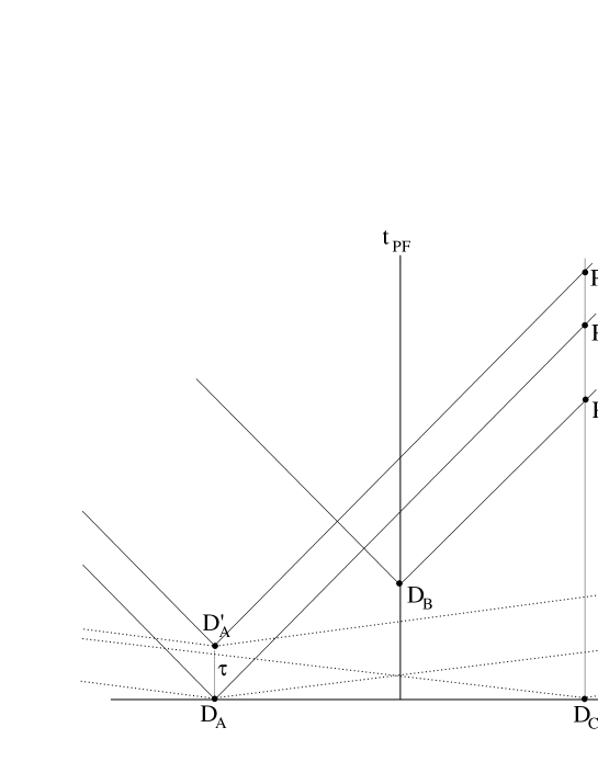
Figure 1: Space-time diagram in the coordinates of the preferred frame (PF) illustrating the non-quantum scenario that leads to conditions (1) and (4). The dots $D$’s are the detection events, the full diagonal lines are standard light cones (cones of classical information), the dotted lines are the ”superluminal communication cones”. See text for the explanation.

As mentioned in the introduction, let’s suppose that the ”reality” underlying quantum correlations consists of local variables (LV) and superluminal communication (SC) with finite speed in a preferred frame (PF). In such a model, when particle A is measured before particle B in the PF, so that SC can go from A to B (that we write A$\rightsquigarrow$B), one recovers the predictions of QM (quantum scenario); and the same is assumed for the reverse time-ordering, B$\rightsquigarrow$A. We suppose moreover that all quantum scenarios are equivalent: as soon as the SC can propagate from one particle to the other, a given source produces always the same statistics, compatible with a quantum state $\rho$.

However, when two particles are measured almost simultaneously in the PF, the SC cannot arrive from one particle to the other (A$\not\leftrightsquigarrow$B). In particular, if in the quantum scenario the probabilities are those computed from the singlet state $\frac{1}{\sqrt{2}}(\mbox{$|01\rangle$}-\mbox{$|10\rangle$})$ and can thus violate Bell’s inequality, then, when A$\not\leftrightsquigarrow$B, these probabilities must be modified in order to become compatible with LV (no Bell inequality violation). Such a loss of non-locality may be testable in an experiment, provided the PF is identified and the sufficient simultaneity is achieved sca ; however, as long as only two particles are concerned, the no-signaling condition does not imply any constraint on the possible models scagisin .

Things are different if we consider three particles A, B and C. Let $P(a,b,c|A,B,C)$ be the statistics of a measurement, where small $x$ are the possible outcomes of the measurement $X$. Whenever the SC can arrive on each link, e.g. A$\rightsquigarrow$B, A$\rightsquigarrow$C and B$\rightsquigarrow$C, the particles give statistics that can be derived from a quantum state $\rho_{ABC}$ (quantum scenario). Whenever a link is broken, e.g. when A$\not\leftrightsquigarrow$C, departures from QM can be expected. In particular, a non-quantum scenario can be constructed in which:

• Particles A and C are measured simultaneously in the preferred frame, hence A$\not\leftrightsquigarrow$C, hence their correlation can be due only to LV:

  $$\mbox{$P(a,c|A,C)$ must come from LV}\,.$$ (1)

  Note that this probability cannot depend on the choice of the measurement on B, since this choice may be done later in time.

• Particle B is measured later, with a time delay sufficient to ensure A$\rightsquigarrow$B and C$\rightsquigarrow$B, but not sufficient to ensure communication at the speed of light to arrive from A or C. It can be shown, see below, that the no-signaling condition requires

  $$\left.\begin{array}[]{lcl}P(a,b|A,B,C)&=&P^{QM}(a,b|A,B)\\ P(b,c|A,B,C)&=&P^{QM}(b,c|B,C)\end{array}\right\}$$ (4)

  where $P^{QM}$ are computed using $\rho_{ABC}$, the state of the source in any quantum scenario.

It is not obvious that conditions (1) and (4) are consistent for any choice of the quantum state, and indeed this will be the main theme of the rest of the paper. Before that, for completeness let us repeat the construction of the scenario, already presented in Ref. scagisin .

The scenario is depicted in Fig. 1. The particles are at locations $x_{A}=-\ell$, $x_{B}=0$ and $x_{C}=+\ell$. The dots $D$’s in the space-time diagram are the detection events. The unprimed events define the non-quantum scenario: as we said, $D_{A}$ and $D_{C}$ are simultaneous and therefore lie outside the SC-cones (dotted lines) of each other, whence condition (1). If A chooses to delay the measurement by a time $\tau$, so that the detection of particle A is now $D^{\prime}_{A}$, the quantum scenario is recovered since C$\rightsquigarrow$A, C$\rightsquigarrow$B and A$\rightsquigarrow$B (follow the SC-cones).

Now, classical information about $D_{B}$ can arrive at the location of C at the point labelled by $P_{BC}$: then, $P(b,c|A,B,C)$ can be estimated. But at that moment, classical information about A has not yet arrived, because it will arrive only in $P_{AC}$ or $P^{\prime}_{AC}$. In particular, the no-signaling condition imposes that $P(b,c|A,B,C)$ cannot depend either on the measurement done on A or on whether that measurement was delayed or not. But if the measurement of A was delayed, we have the quantum scenario, so in particular $P(b,c|A,B,C)=P^{QM}(b,c|B,C)$ as required in (1). The other part of (1), $P(a,b|A,B,C)=P^{QM}(a,b|A,B)$ can be derived by the symmetric argument, supposing that it is C that can delay the measurement (situation not shown in the figure, for clarity).

III The need for local variables

A first instructive step is taken by supposing that there are no LV at all, that is, all the correlations are due to SC. In this case, condition (1) is replaced by the stronger condition of independence:

$$P(a,c|A,B,C) = P^{QM}(a|A)P^{QM}(c|C)$$ (5)

where the marginals must be those of QM to avoid signaling. Now, it is very easy to see that this condition and condition (4) are incompatible. Consider a source that produces, in the quantum scenarios, the Greenberger-Horne-Zeilinger state of three qubits $\mbox{$|GHZ\rangle$}=\frac{1}{\sqrt{2}}\big{(}\mbox{$|000\rangle$}+\mbox{$|111\rangle$}\big{)}$, and suppose that all three measurements are $A=B=C=\sigma_{z}=\mbox{$|0\rangle$}\mbox{$\langle 0|$}-\mbox{$|1\rangle$}\mbox{$\langle 1|$}$. Then condition (4) leads to $P(a=b)=1$ and $P(b=c)=1$; but if $a$ is always equal to $b$ and $b$ is always equal to $c$, then $P(a=c)=1$ should hold as well, in contradiction with (5) that predicts $P(a=c)=P(a\neq c)=\frac{1}{2}$. We have thus proved

Theorem 1. In any model of superluminal communication with finite speed, the assumption that there are no local variables leads to signaling.

In some sense, the result of this paragraph is the counterpart of Bell’s theorem for the SC-models that we consider: SC with finite speed cannot be alone the cause of quantum correlations, some LV must be present as well. This was proved in scagisin . In the next paragraph, we extend this result by showing that a well-defined class of LV model is not enough to restore the no-signaling condition.

IV The need for non-quantum statistics

We can go a step further and require that $P(a,b,c|A,B,C)$ can always be obtained from a quantum state. This would mean that, when we arrange a situation in which particles A and C do not communicate, the statistics are still described by a density matrix $\tilde{\rho}_{ABC}$ such that the partial state $\tilde{\rho}_{AC}$ can be described by LV in order to satisfy (1). This extension is enough to remove signaling from the example of the GHZ state described just above: the LV statistics may be those of the quantum state $\tilde{\rho}_{ABC}=\frac{1}{2}P_{000}+\frac{1}{2}P_{111}$. However, moving to other quantum states we can demonstrate the following:

Theorem 2. In any model of superluminal communication with finite speed, the requirement that $P(a,b,c|A,B,C)$ can always be obtained from a quantum state leads to signaling.

This follows from a result by Linden and Wootters linden applied to our situation. At least two qubits and one qutrit are needed to work out this argument. Consider the state in $\begin{picture}(8.0,8.0)\put(0.0,0.0){C}\put(3.0,0.3){\line(0,1){7.0}}\end{picture}^{2}\otimes\begin{picture}(8.0,8.0)\put(0.0,0.0){C}\put(3.0,0.3){\line(0,1){7.0}}\end{picture}^{3}\otimes\begin{picture}(8.0,8.0)\put(0.0,0.0){C}\put(3.0,0.3){\line(0,1){7.0}}\end{picture}^{2}$

$$|\Psi\rangle = \cos\alpha\,\frac{\mbox{$|021\rangle$}+\mbox{$|120\rangle$}}{\sqrt{2}}\,+\,\sin\alpha\,\frac{\mbox{$|000\rangle$}+\mbox{$|111\rangle$}}{\sqrt{2}}$$ (6)

with $0<\alpha<\frac{\pi}{2}$. The statistics of the sub-systems A-B and B-C are computed from the density matrices

$$\rho_{AB}=\rho_{CB} = \frac{1}{2}\mbox{$|\psi_{1}\rangle$}\mbox{$\langle\psi_{1}|$}\,+\,\frac{1}{2}\mbox{$|\psi_{2}\rangle$}\mbox{$\langle\psi_{2}|$}$$ (7)

where $\mbox{$|\psi_{1}\rangle$}=\sin\alpha\mbox{$|00\rangle$}+\cos\alpha\mbox{$|12\rangle$}$ and $\mbox{$|\psi_{2}\rangle$}=\sin\alpha\mbox{$|11\rangle$}+\cos\alpha\mbox{$|02\rangle$}$. The statistics of the two qubits A-C is computed from

$$\rho_{AC} = \cos^{2}\alpha\mbox{$|\Psi^{+}\rangle$}\mbox{$\langle\Psi^{+}|$}\,+\,\frac{\sin^{2}\alpha}{2}\,\left(P_{00}+P_{11}\right)$$ (8)

and violates the Clauser-Horne-Shimony-Holt (CHSH) inequality for $\cos^{2}\alpha>\frac{1}{\sqrt{2}}$ chsh . We want to show that $|\Psi\rangle$ is the only quantum state of A-B-C, pure or mixed, compatible with the partial traces (7).

Here is the proof. One starts from $\rho_{AB}$ given by (7): since $|\psi_{1}\rangle$ and $|\psi_{2}\rangle$ are orthogonal, any purification of $\rho_{AB}$ can be written

$$|\Phi\rangle = \frac{1}{\sqrt{2}}\big{(}\mbox{$|\psi_{1}\rangle$}_{AB}\mbox{$|E_{1}\rangle$}_{CX}+\mbox{$|\psi_{2}\rangle$}_{AB}\mbox{$|E_{2}\rangle$}_{CX}\big{)}$$ (9)

with $X$ an auxiliary mode and $\mbox{$\langle E_{1}|E_{2}\rangle$}=0$. Then, using the Schmidt decomposition:

$$\mbox{$|E_{1}\rangle$}_{CX} = c_{0}\mbox{$|0\rangle$}_{C}\mbox{$|x_{10}\rangle$}_{X}+c_{1}\mbox{$|1\rangle$}_{C}\mbox{$|x_{11}\rangle$}_{X}$$ (10)

$$\mbox{$|E_{2}\rangle$}_{CX} = d_{0}\mbox{$|0\rangle$}_{C}\mbox{$|x_{20}\rangle$}_{X}+d_{1}\mbox{$|1\rangle$}_{C}\mbox{$|x_{21}\rangle$}_{X}$$ (11)

with $\mbox{$\langle x_{k0}|x_{k1}\rangle$}=0$. The rest of the proof goes as follows: one inserts these expressions into $|\Phi\rangle$, and then requires that $\rho_{BC}$ is also given by (7). Specifically, $\rho_{BC}$ should span a space that is orthogonal to $\mbox{$|01\rangle$}_{BC}$ and $\mbox{$|10\rangle$}_{BC}$. By direct inspection, for $0<\alpha<\frac{\pi}{2}$, this forces $c_{1}=d_{0}=0$, that in turn implies $c_{0}=d_{1}=1$. Using this condition, one can further verify that $\rho_{BC}$ can be obtained only if $\mbox{$\langle x_{10}|x_{21}\rangle$}=1$. All in all, this implies means that

$$\mbox{$|\Phi\rangle$}_{ABCX} = \mbox{$|\Psi\rangle$}_{ABC}\mbox{$|x\rangle$}_{X}\,:$$ (12)

$\mbox{$|\Psi\rangle$}_{ABC}$ is the only quantum state, pure or mixed, compatible with the quantum marginals (7). In particular then, fixing $\rho_{AB}$ and $\rho_{BC}$ as required by the no-signaling condition (4) implies that $P(a,c|A,B,C)$ is the statistics derived from $\rho_{AB}$. For $\cos^{2}\alpha>\frac{1}{\sqrt{2}}$, this is non-local, in contradiction with the spirit of the model (1).

In conclusion: if, in addition to conditions (1) and (4), we impose that the possible probabilities must still be describable within quantum physics, then we reach a contradiction. Thus, if one wants to invoke finite-speed superluminal communication to describe quantum correlations and, at the same time, avoid superluminal signaling between observers, the only hope left lies with local variables distributed according to non-quantum statistics.

V Most general model

The additional constraints that we imposed in the previous sections (no LV, then LV coming from a density matrix) are good working hypotheses, but rather artificial. If one is ready to allow a departure from quantum physics by assuming the finiteness of the ”speed of quantum information”, then one is also ready to accept the most general local variable models to describe the situations where the information is not arrived. Can one still find a contradiction in this extended framework? That is, are conditions (1) and (4) definitely contradictory, without any further hypothesis? The answer is, we don’t know. What we do know, is that non-quantum local variables are enough to remove the contradiction pinpointed in the previous section, based on the specific state (6).

To prove this statement, the starting point is to have a convenient form for the probabilities. Since A and C give binary outcomes, we can label these outcomes $a,c=\pm 1$. It is easy to be convinced that any probability distribution of two bits and another variable (here, the trit $b$) can be written as

$$P(a,b,c|M) = \frac{1}{4}\,\Big{[}F_{M}(b)\,+\,a\,A_{M}(b)$$ (13)

$$+\,c\,C_{M}(b)\,+\,ac\,H_{M}(b)\Big{]}$$

where $M=\{A,B,C\}$ labels the measurements and where the functions introduced here are submitted to the constraint that all probabilities must be positive and sum up to one. Note in particular that $\sum_{b}F_{M}(b)=1$. In this notation, the correlation coefficient A-C is given by

$$E(ac|M) = \sum_{b}H_{M}(b)\,.$$ (14)

Condition (4) implies directly that $F_{M}$, $A_{M}$ and $C_{M}$ must be those that can be computed in QM, and that the only freedom for an alternative model is left on $H_{M}$.

We have to estimate the constraints that are imposed on $E(ac|M)$. For this, we fix once for all the measurements on the qubits. At first, we fix also the measurement $B$ and its result $b$. Any value of $H_{M}$ is acceptable that satisfies the condition that all the probabilities are non-negative:

$$\left.\begin{array}[]{lcl}P(+,b,+)&=&F_{M}+A_{M}+C_{M}+H_{M}\geq 0\\ P(-,b,-)&=&F_{M}-A_{M}-C_{M}+H_{M}\geq 0\end{array}\right\}$$ (17)

$$\left.\begin{array}[]{lcl}P(+,b,-)&=&F_{M}+A_{M}-C_{M}-H_{M}\geq 0\\ P(-,b,+)&=&F_{M}-A_{M}+C_{M}-H_{M}\geq 0\end{array}\right\}$$ (20)

From (17) we obtain the lower bound $H_{M}\,\geq\,-F_{M}(b)+|A_{M}(b)+C_{M}(b)|\equiv L_{M}(b)$, from (20) the upper bound $H_{M}\,\leq\,F_{M}(b)-|A_{M}(b)-C_{M}(b)|\equiv U_{M}(b)$. In conclusion, for $B$ and its outcome fixed, all the values of $H$ are possible that satisfy

$$L_{M}(b)\,\leq H_{M}(b) \leq\,U_{M}(b)\,.$$ (21)

From this last equation, using (14), we can immediately derive the consequent constraint on the A-C correlations:

$$\sum_{b}L_{M}(b)\equiv L_{M} \leq E(ac|M)\leq U_{M}\equiv\sum_{b}U_{M}(b)\,.$$ (22)

Remember that the source is such that $E(ac|M)$ violates the CHSH inequality for suitable settings in the quantum scenario; our goal is to see whether the bounds we have just derived are tight enough to preserve the violation. Let $M_{ij}=\{A_{i},B,C_{j}\}$ for $i,j=1,2$: the CHSH inequality reads $|{\cal{B}}|\leq 2$ where

$${\cal{B}} = E(ac|M_{11})+E(ac|M_{12})$$ (23)

$$+E(ac|M_{21})-E(ac|M_{22})\,.$$

The bounds (22) impose the following constraints:

$${\cal{B}} \geq {\cal{L}}\equiv L_{11}+L_{12}+L_{21}-U_{22}$$ (24)

$${\cal{B}} \leq {\cal{U}}\equiv U_{11}+U_{12}+U_{21}-L_{22}$$ (25)

where $L_{ij}\equiv L_{M_{ij}}$ and $U_{ij}\equiv U_{M_{ij}}$. Thus, the constraints under study force the violation of CHSH if and only if there exist a family of four measurements $\{M_{ij}\}$ such that either ${\cal{L}}>2$ or ${\cal{U}}<-2$ holds.

To check this for the state (6), we recall that the functions $F_{M}(b)$, $A_{M}(b)$ and $C_{M}(b)$ must be those predicted by QM. Specifically, let $\mbox{$|b\rangle$}=b_{0}\mbox{$|0\rangle$}+b_{1}\mbox{$|1\rangle$}+b_{2}\mbox{$|2\rangle$}$ the eigenstate of measurement $B$ for the eigenvalue $b$; and the parametrization of the measurements on the two qubits be given in terms of the vectors in the Bloch sphere $\hat{n}_{X}=(\theta_{X},\varphi_{X})$ for $X=A,C$. Then we compute $P^{QM}(a,b,c|M)=\big{|}\mbox{$\langle a\hat{n}_{A},b,c\hat{n}_{C}|\Psi\rangle$}\big{|}^{2}$, write it down in the form (13) and thus find

$$F_{M}(b) = \cos^{2}\alpha\,|b_{2}|^{2}+\frac{1}{2}\sin^{2}\alpha\,(1-|b_{2}|^{2})\,,$$

$$A_{M}(b) = \frac{1}{2}\sin^{2}\alpha\cos\theta_{A}(|b_{0}|^{2}-|b_{1}|^{2})$$

$$+\frac{1}{2}\sin 2\alpha\sin\theta_{A}\,\mbox{Re}\big{[}e^{i\varphi_{A}}(b_{0}b_{2}^{*}+b_{2}b_{1}^{*})\big{]}\,,$$

$$C_{M}(b) = \frac{1}{2}\sin^{2}\alpha\cos\theta_{C}(|b_{0}|^{2}-|b_{1}|^{2})$$

$$+\frac{1}{2}\sin 2\alpha\sin\theta_{C}\,\mbox{Re}\big{[}e^{i\varphi_{C}}(b_{0}b_{2}^{*}+b_{2}b_{1}^{*})\big{]}$$

The last step is to maximize ${\cal{L}}$ (respectively minimize ${\cal{U}}$) over all possible families of four measurements $\{M_{ij}\}$. This is an optimization over fourteen real parameters: four for qubit A ($\theta_{A_{i}}$ and $\varphi_{A_{i}}$ for $i=1,2$), as much for qubit C (the analog ones), and six for the qutrit B, the number of real parameters needed to define a basis, i.e. an element of $SU(3)$. We programmed the optimization in Matlab. The result is that ${\cal{L}}$ is always clearly smaller than 2 for any value of $\alpha$. Specifically, $\bar{{\cal{L}}}=\max_{\{M\}}{\cal{L}}$ starts at $-4$ for $\alpha=0$, then increases to $\sim 0.4$ at the point $\cos^{2}\alpha=\frac{1}{\sqrt{2}}$ where the quantum state $\rho_{AB}$ ceases to violate the CHSH inequality, and finally reaches exactly 2 for $\alpha=\frac{\pi}{2}$, that is $\mbox{$|\Psi\rangle$}=\mbox{$|GHZ\rangle$}$. As intuitively expected, ${\cal{U}}$ behaves exactly in the symmetric way: $\bar{{\cal{U}}}=\min_{\{M\}}{\cal{U}}$ starts at 4 for $\alpha=0$ and decreases down to $-2$ for $\alpha=\frac{\pi}{2}$ note2 .

Let’s summarize: we have studied a state that is entirely determined by its ”quantum marginals” $\rho_{AB}$ and $\rho_{BC}$ if we want to stay within quantum mechanics. However, if we relax this requirement, several non-quantum functions $H_{M}(b)$ become possible — that quantum probabilities have much built-in structure is evident e.g. from the fact that $H_{M}(b)$ must be bilinear in the vectors $\hat{n}_{A}$ and $\hat{n}_{C}$ in the quantum case, while in the non-quantum case $H_{M}(b)$ need not even be a continuous function of these vectors. All this freedom is enough to break the uniqueness result that holds in the quantum case, so strongly, that also the non-locality of the marginal distribution A-C is destroyed. Thus, for the state (6) that we have considered and for the CHSH inequality, superluminal communication with finite speed does not lead to signaling when non-quantum local variables are allowed. It remains an open problem to determine whether this conclusion holds in general, whatever the state and for any possible Bell-type inequality.

VI Discussion

We have put constraints on the possibility of using superluminal communication with finite speed to describe quantum correlations. Specifically, local variables that yield intrinsically non-quantum statistics must be provided together with this communication mechanism, in order to avoid signaling. Whether ultimately such non-quantum local variables lead to signaling too — thus ruling out all models based on finite-speed superluminal communication — is still an open question; we sketched a possible approach to tackle it. The constraints discussed in this paper should contribute to inspire deeper models for ”emergent quantum mechanics”.

References

- (1) For some examples, see: S.L. Adler, Quantum Theory as an Emergent Phenomenon (Cambridge University Press, Cambridge, 2004); G. ’t Hooft, quant-ph/0212095; F. Markopoulou, L. Smolin, gr-qc/0311059; and several papers in these Proceedings.
- (2) A. Einstein, B. Podolski, N. Rosen, Phys. Rev. 47, 777 (1935)
- (3) J.S. Bell, Speakable and Unspeakable in Quantum Mechanics: Collected papers on quantum philosophy (Cambridge University Press, Cambridge, 1987)
- (4) D. Bohm, B.J. Hiley, The undivided universe (Routledge, New York, 1993)
- (5) Ph. Eberhard, A Realistic Model for Quantum Theory with a Locality Property, in: W. Schommers (ed.), Quantum Theory and Pictures of Reality (Springer, Berlin, 1989)
- (6) T. Durt, Helv. Phys. Acta 72, 356 (1999)
- (7) A. Suarez, V. Scarani, Phys. Lett. A 232, 9 (1997). This model was also ruled out by experiment: H. Zbinden, J. Brendel, N. Gisin, W. Tittel, Phys. Rev. A 63, 022111 (2001); A. Stefanov, H. Zbinden, N. Gisin, A. Suarez, Phys. Rev. Lett. 88, 120404 (2002)
- (8) V. Scarani, N. Gisin, Phys. Lett. A 295, 167 (2002)
- (9) Experimental lower bounds for this speed have been presented in: V. Scarani, W. Tittel, H. Zbinden, N. Gisin, Phys. Lett. A 276, 1 (2000)
- (10) One might ask why the no-signaling condition should be enforced if we assume a preferred frame for quantum phenomena. Indeed, there is no longer a fundamental reason for that requirement. Still, classical events seem to be conveniently described using special relativity; and the record of a detection is a classical events that can be precisely located in space-time.
- (11) N. Linden, W.K. Wootters, Phys. Rev. Lett. 89, 277906 (2002)
- (12) J.F. Clauser, M.A. Horne, A. Shimony, R.A. Holt, Phys. Rev. Lett. 23, 880 (1969). To compute the maximal violation and the corresponding settings, see: R. Horodecki, P. Horodecki, M. Horodecki, Phys. Lett. A 200, 340 (1995)
- (13) Obviously, although for some values of it happens that , for any given set of measurements holds.