Abstract

In ghost imaging schemes information about an object is extracted by measuring the correlation between a beam that passed the object and a reference beam. We present a spatial averaging technique that substantially improves the imaging bandwidth of such schemes, which implies that information about high-frequency Fourier components can be observed in the reconstructed diffraction pattern. In the many-photon regime the averaging can be done in parallel and we show that this leads to a much faster convergence of the correlations. We also consider the reconstruction of the object image, and discuss the differences between a pixel-like detector and a bucket detector in the object arm. Finally, it is shown how to non-locally make spatial filtering of a reconstructed image. The results are presented using entangled beams created by parametric down-conversion, but they are general and can be extended also to the important case of using classically correlated thermal-like beams.

OCIS codes: (270.0270) Quantum optics, (110.0110) Imaging systems, (190.0190) Nonlinear optics, (100.0100) Image processing.

1 Introduction

Lately a substantial effort has been put into understanding the physics behind “ghost” imaging [1, 2, 3, 4, 5, 6, 7, 8, 9, 10, 11, 12, 13], also called entangled imaging, two-photon imaging, coincidence imaging, or correlated imaging. The ghost imaging schemes are based on two correlated beams typically originating from parametric down conversion (PDC). One beam travels a path (the test arm) containing an unknown object, while the other beam is sent through a reference optical system (the reference arm). Information about the object is then obtained by measuring the spatial correlation between the beams. This two-arm configuration allows for obtaining different kinds of information by solely operating on the reference arm optical setup while keeping the test arm fixed. In particular, both the image (near-field distribution) and the diffraction pattern (far-field distribution) of the object can be measured [9].

The early studies concentrated on the working principles of the ghost imaging scheme, both in terms of basic formalism [1, 2] as well as the experimental implementation [3, 4, 5]. A general theory has been developed that discusses how to extract the information, not only in the coincidence counting regime [6, 7, 8], but also in the high gain regime [9, 10, 11, 12] where recent experimental results showed nonclassical spatial correlations for for high-gain PDC [14], which promises well for an efficient quantum ghost imaging protocol. Most recent discussions have instead focused on whether entanglement is necessary for extracting the information [6, 7, 8, 9, 10, 11, 13] and references therein. The present paper focuses on how to optimize any source, entangled or not, to give as much image information as possible. The issues of imaging bandwidth and image resolution have been taken up previously [9, 10, 11, 12, 13]. Even in an ideal ghost imaging system the imaging bandwidth is limited by the source generating the correlated beams, characterized by a finite extension of the spatial gain in Fourier space $\delta q_{\rm source}$: beyond this value the Fourier frequencies are cut off and this information is lost in the reconstruction of the object diffraction pattern. The image resolution is instead limited by the coherence length $x_{\mathrm{coh}}$, which is given by the characteristic width of the near-field correlation function.

The question is: can we increase the source cutoff value? In the case of PDC the cutoff is determined by the phase-matching conditions [15, 10, 12] while in the case of a classically correlated field generated from chaotic thermal radiation, the bandwidth is roughly given by the inverse of speckle size found from the self-interference of the near field [16] (see also [10, 13]). Thus, the cutoff is an inherent property of the source. However, in this paper we discuss a spatial averaging technique which circumvents this cutoff and improves the imaging bandwidth of the system, regardless of how the correlated beams are created. The spatial average is performed over the position of a pixel-like detector located in the test arm after the object, exploiting that each position of this detector gives access to a different part of the diffraction pattern through the correlations. Thus, making an average over all possible positions of the test detector it is possible to substantially extend the imaging bandwidth of the scheme.

The spatial averaging technique works particularly well in the high-gain regime where many photon pairs are generated in each pump pulse. Thus the test arm has many photons per pulse transmitted by the object, (in contrast in the low-gain coincidence counting regime only one photon at a time is impinging on the object, and either it is transmitted or it is not), and therefore at the measurement plane they are scattered over the entire transverse plane. The information about the object is then extracted by spatially correlating the intensities recorded in the test and reference arm. In the low-gain regime this implies registering coincidences while in the high gain regime successive sampling over repeated shots of the pump pulse is used. Since the spatial averaging technique employs an average over the position of the test detector, within a single shot we can get information about the image from all the test detector positions in the transverse plane containing photons. This implies that in the high gain regime a much faster convergence rate is obtained using the spatial averaging technique.

The spatial averaging technique was already introduced in Ref. [12] in the case where homodyne detection was used. Since the homodyne measurements give access to orthogonal quadratures, an increased image resolution can be obtained by using the spatial averaging technique to measure the diffraction pattern and then use an inverse Fourier transform to obtain the image. In the present work we only have access to the field intensity, so we cannot use this method to get an increased image resolution. However, we may use a bucket detector in the test arm when we want to observe the image, which was not possible in the homodyne scheme due to phase-control problems, and it turns out to make the imaging system incoherent. We discuss the benefits and disadvantages in this respect. We will also extend the discussion of [12] and give a more detailed and general picture as to why the spatial averaging technique works, and as to how much the convergence rate can be improved.

The majority of the results of this paper hold for ghost imaging schemes in general, however we use in the following a model for PDC as the source for the correlated beams.

The paper starts by presenting the analytical results in Sec. 2, and the spatial averaging scheme is introduced and discussed. The numerical results are contained in Sec. 3, going beyond the approximations made in the analytical section and validating the results by using very realistic parameters of current experiments. The paper is summarized in Sec. 4.

2 The model and analytical results

We consider the PDC model for the three-wave quantum interaction inside a $\chi^{(2)}$ nonlinear crystal previously discussed in detail in Refs. [12, 15]. The crystal of length $l_{\rm c}$ is cut for type II phase matching, and the model consists of a set of operator equations describing the evolution inside the crystal of the quantum mechanical boson operators $a_{j}({\bf x},z,t)$ for the signal ($j=1$) and idler ($j=2$) fields, obeying at a given $z$ the commutator relations $[a_{i}(z,{\bf x},t),a_{j}^{{\dagger}}(z,{\bf x}^{\,\prime},t^{\prime})]=\delta_{ij}\delta({\bf x}-{\bf x}^{\,\prime})\delta(t-t^{\prime})$, $i,j=1,2$. In the stationary and plane-wave pump approximation (SPWPA) unitary input-output transformations can be written relating the field operators in ${\bf q}$ and $\Omega$ space at the output face of the crystal $b_{j}({\bf q},\Omega)\equiv a_{j}(z=l_{\rm c},{\bf q},\Omega)$ to those at the input face $a_{j}^{\mathrm{in}}({\bf q},\Omega)\equiv a_{j}(z=0,{\bf q},\Omega)$ as follows

$$b_{j}({\bf q},\Omega)=U_{j}({\bf q},\Omega)a_{j}^{\mathrm{in}}({\bf q},\Omega)+V_{j}({\bf q},\Omega)a_{k}^{\mathrm{in{\dagger}}}(-{\bf q},-\Omega),\quad j\neq k=1,2.$$ (1)

The gain functions $U_{j}$ and $V_{j}$ can for example be found in [12, 15].

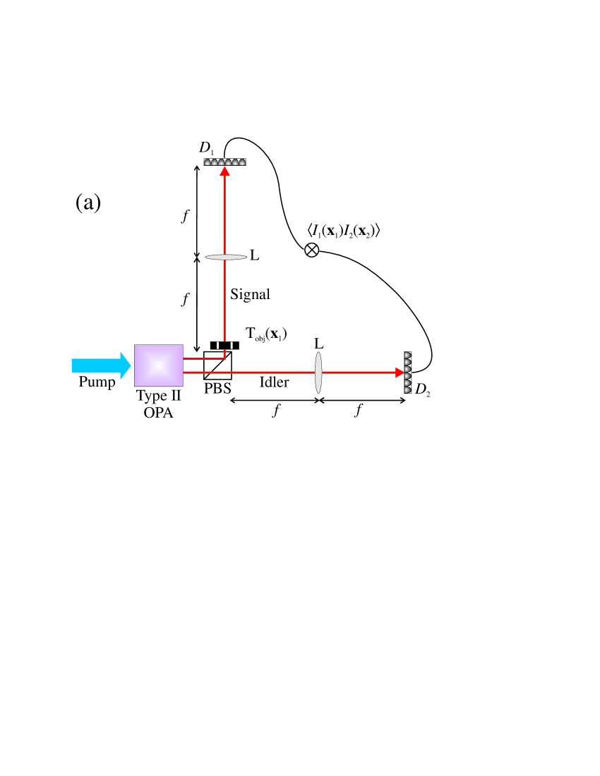
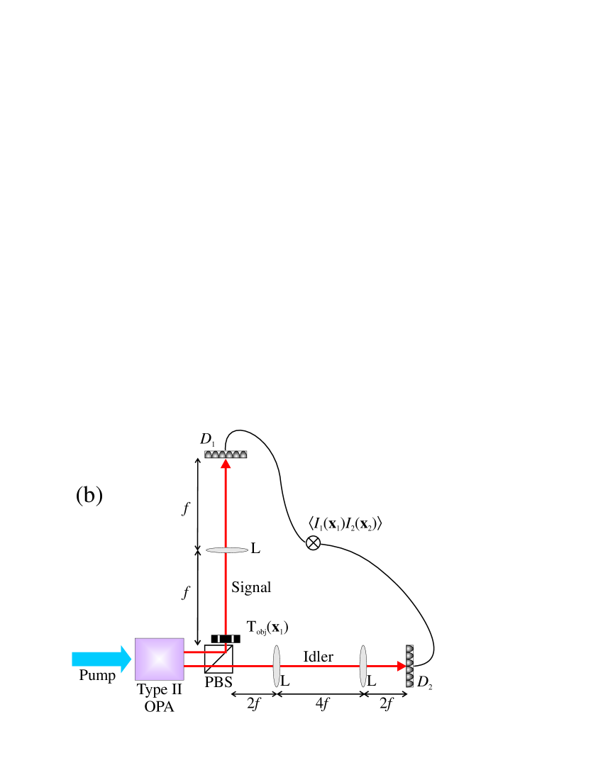
Fig. 1: System setup. In (a) the setup for reconstructing the diffraction pattern of the object is shown, where the reference arm is in the f-f setup. In (b) the reference arm is changed to a telescope setup, which is used to reconstruct the object near field. PBS: polarizing beam splitter. L: lens of focal length $f$. $T_{\rm obj}$: object. $D_{1}$, $D_{2}$: arrays of detectors.

The system setup we consider is the same as in Refs. [9, 10, 11, 12] and has the characteristic two-arm configuration of the ghost imaging scheme, see Fig. 1. The signal and idler exiting from the crystal are separated with a polarizing beam splitter (PBS). The object is located in the test (signal) arm immediately after the PBS, and the transmitted field then propagates through an f-f lens system: a lens placed distance $f$ from the object as well as to the measurement plane, where $D_{1}$ (an array of pixels or a CCD camera) is recording the intensity of the field. Thus $D_{1}$ is in the focal plane of the lens, but it is important to stress that it cannot on its own measure the interference pattern of the object because the signal beam itself is incoherent. This test arm setup is kept fixed, while in the reference (idler) arm two different configurations are used. In Fig. 1(a) the reference arm contains also an f-f lens system, and by recording the idler field intensity with $D_{2}$ (another CCD camera) and correlating it with the signal intensity, information about the object diffraction pattern can be extracted from the correlations. Conversely, in Fig. 1(b) a so-called telescope setup is used consisting of two lenses with focal length $f$ placed 4$f$ from each other and $2f$ from the PBS and $D_{2}$, respectively. This setup allows for retrieval of the object image distribution from the correlations.

The analytical results for the correlations in the two cases of Fig. 1 were derived in Ref. [9, 10], and we review them in the following. For simplicity we neglect for the moment the temporal argument, which corresponds to using a narrow frequency filter after the crystal. The propagation of the fields from the PBS to the measurement planes are described by the kernels $h_{j}({\bf x}_{j},{\bf x}^{\,\prime}_{j})$. The fields at the measurement plane $c_{j}({\bf x}_{j})$ are then found by the Fresnel transformation $c_{j}({\bf x}_{j})=\int{\rm d}{\bf x}^{\,\prime}_{j}h_{j}({\bf x}_{j},{\bf x}^{\,\prime}_{j})b_{j}({\bf x}^{\,\prime}_{j})+L_{j}({\bf x}_{j})$. $L_{j}({\bf x}_{j})$ represent the losses in the propagation which are proportional to the vacuum field operators and are uncorrelated from $b_{j}({\bf x}_{j})$. The field intensities at the measurement planes $I_{j}({\bf x}_{j})=c_{j}^{\dagger}({\bf x}_{j})c_{j}({\bf x}_{j})$ are detected with $D_{j}$, and result in the correlation $\langle I_{1}({\bf x}_{1})I_{2}({\bf x}_{2})\rangle=\langle c_{1}^{\dagger}({\bf x}_{1})c_{1}({\bf x}_{1})c_{2}^{\dagger}({\bf x}_{2})c_{2}({\bf x}_{2})\rangle$. The information about the object is obtained by subtracting the background term to obtain the intensity fluctuation correlations

$$G({\bf x}_{1},{\bf x}_{2})=\langle I_{1}({\bf x}_{1})I_{2}({\bf x}_{2})\rangle-\langle I_{1}({\bf x}_{1})\rangle\langle I_{2}({\bf x}_{2})\rangle.$$ (2)

It is then straightforward to show the following essential result [9, 10]

$$G({\bf x}_{1},{\bf x}_{2})=\left|\int{\rm d}{\bf x}^{\,\prime}_{1}\int{\rm d}{\bf x}^{\,\prime}_{2}h_{1}({\bf x}_{1},{\bf x}^{\,\prime}_{1})h_{2}({\bf x}_{2},{\bf x}^{\,\prime}_{2})\Gamma({\bf x}^{\,\prime}_{1}-{\bf x}^{\,\prime}_{2},\Omega=0)\right|^{2},$$ (3)

Here $\Gamma({\bf x}_{1},{\bf x}_{2},\Omega)$ is the near-field correlation at the crystal exit, and in the SPWPA and with $a_{j}^{\mathrm{in}}$ in the vacuum state it is found from Eq. (1) as

$$\Gamma({\bf x}_{1},{\bf x}_{2},\Omega)\equiv\int{\rm d}\tau e^{-i\Omega\tau}\langle b_{1}({\bf x}_{1},t_{1})b_{2}({\bf x}_{2},t_{1}+\tau)\rangle=\int\frac{{\rm d}{\bf q}}{(2\pi)^{2}}e^{i{\bf q}\cdot({\bf x}_{1}-{\bf x}_{2})}\gamma({\bf q},\Omega)\>,$$ (4)

where we have introduced the gain function $\gamma({\bf q},\Omega)=U_{1}({\bf q},\Omega)V_{2}(-{\bf q},-\Omega)$. Since Eq. (4) is a function of ${\bf x}_{1}-{\bf x}_{2}$ (because of the SPWPA) we will use the notation $\Gamma({\bf x}_{1}-{\bf x}_{2},\Omega)=\Gamma({\bf x}_{1},{\bf x}_{2},\Omega)$ in the following.

We should mention that when temporal argument is taken into account, Eq. (3) is no longer valid. We consider the intensities averaged over the detection time $T_{\rm D}$ as $I_{j}({\bf x}_{j})=T_{\rm D}^{-1}\int_{T_{\rm D}}{\rm d}tc_{j}^{\dagger}({\bf x}_{j},t)c_{j}({\bf x}_{j},t)$. When $T_{\rm D}$ is much larger than the coherence time of the source $\tau_{\rm coh}$ (which for PDC is typically the case) the following expression holds instead [11]

$$G({\bf x}_{1},{\bf x}_{2})=\frac{1}{T_{\rm D}}\int\frac{{\rm d}\Omega}{2\pi}\left|\int{\rm d}{\bf x}^{\,\prime}_{1}\int{\rm d}{\bf x}^{\,\prime}_{2}h_{1}({\bf x}_{1},{\bf x}^{\,\prime}_{1})h_{2}({\bf x}_{2},{\bf x}^{\,\prime}_{2})\Gamma({\bf x}^{\,\prime}_{1}-{\bf x}^{\,\prime}_{2},\Omega)\right|^{2}.$$ (5)

This form will be used later for comparing with the numerics.

We fix the test arm once and for all as shown in Fig. 1, so $h_{1}({\bf x}_{1},{\bf x}^{\,\prime}_{1})\propto e^{-i{\bf x}_{1}\cdot{\bf x}^{\,\prime}_{1}k/f}T_{\rm obj}({\bf x}^{\,\prime}_{1})$, where $k$ is the free space wave number of the degenerate down-converted fields. To extract information about the diffraction pattern the reference arm is set in the f-f setup of Fig. 1(a), $h_{2}({\bf x}_{2},{\bf x}^{\,\prime}_{2})\propto e^{-i{\bf x}_{2}\cdot{\bf x}^{\,\prime}_{2}k/f}$, and Eq. (3) then straightforwardly implies the correlation [9, 10, 11]

$$G_{\rm{f}}({\bf x}_{1},{\bf x}_{2})\propto\left|\gamma(-{\bf x}_{2}k/f,\Omega=0)\,\tilde{T}_{\rm obj}\left[({\bf x}_{1}+{\bf x}_{2})k/f\right]\right|^{2}\>,$$ (6)

where $\tilde{T}_{\rm obj}({\bf q})=\int\frac{{\rm d}{\bf x}}{2\pi}e^{-i{\bf q}\cdot{\bf x}}T_{\rm obj}({\bf x})$ is the amplitude of the object diffraction pattern. The subscript “f” denotes that the reference arm is in the f-f configuration. The correlation provides information about the diffraction pattern of the object if we fix ${\bf x}_{1}$ and scan ${\bf x}_{2}$, but since the gain also depends on ${\bf x}_{2}$ there is a limit to the information we can extract. Precisely, the gain $\gamma(-{\bf x}_{2}k/f,\Omega=0)$ introduces a cutoff of the reproduced spatial Fourier frequencies at a certain characteristic value which we denote $\delta q_{\rm PDC}$; the imaging bandwidth of the PDC source.

We will now show how to circumvent this source-related limitation on the imaging bandwidth. As previously shown [12] we may in a suitable way average over the position of the test arm detector ${\bf x}_{1}$: First, a change of variables is introduced as ${\bf x}\equiv{\bf x}_{1}+{\bf x}_{2}$, and then an average over ${\bf x}_{1}$ is performed. We then obtain

$$G_{\mathrm{f},{\rm SA}}({\bf x})\equiv\int{\rm d}{\bf x}_{1}G_{\mathrm{f}}({\bf x}_{1},{\bf x}-{\bf x}_{1})\propto\int{\rm d}{\bf x}_{1}\left|\gamma[({\bf x}_{1}-{\bf x})k/f,\Omega=0]\,\tilde{T}_{\rm obj}({\bf x}k/f)\right|^{2}$$

$$=|\tilde{T}_{\rm obj}({\bf x}k/f)|^{2}\int{\rm d}{\bf x}_{1}\left|\gamma[({\bf x}_{1}-{\bf x})k/f,\Omega=0]\right|^{2}\simeq{\rm const}\times|\tilde{T}_{\rm obj}({\bf x}k/f)|^{2}$$ (7)

where the subscript “SA” indicates that a spatial average has been carried out. The final approximation in (7) is that $|\gamma({\bf q},\Omega=0)|^{2}$ is a bound function inside the detection range of ${\bf x}_{1}$ implying that the integral evaluates to a constant. Thus, there is now no gain cutoff of the diffraction pattern, so the imaging bandwidth becomes practically infinite (apart from limitations arising from the finite size of the optical elements). Note that this average over ${\bf x}_{1}$ does not correspond to $D_{1}$ being a bucket detector. Instead, the change in variables ${\bf x}\equiv{\bf x}_{1}+{\bf x}_{2}$ implies that the spatial averaging technique is a convolution of the signal and idler intensity fluctuations, which in practice is easily calculated using fast Fourier transform techniques.

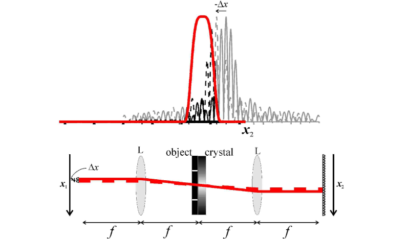
Fig. 2: The spatial averaging technique explained by the Klyshko picture. The lower sketch shows the unfolded version of Fig. 1(a). The red line represents the ray from the detector at position $x_{1}^{0}$ as it travels through the system and reaches its conjugate point in the reference plane on the right side. The upper plot shows the source gain curve in Fourier space and the position of a typical diffraction pattern for the current value of $x_{1}^{0}$; only the black part is amplified while the gray part is not amplified. As the test detector position is changed to $x_{1}^{0}+\Delta x$ the dashed red ray comes into play, and the diffraction pattern in the upper plot moves a corresponding amount (also dashed). The gain instead remains the same, and hence a different part of the diffraction pattern is amplified. (Movie size 449 KB).

In Fig. 2 we give an intuitive explanation of why the bandwidth is extended by averaging over ${\bf x}_{1}$, and it is based on the Klyshko picture [1] (see also [17]). This states that the propagation in the two distinct arms can be viewed in an “unfolded” scheme having the nonlinear crystal as the hinge point of the signal and idler rays, i.e. the crystal can be treated as a geometrical reflection mirror. This is a consequence of momentum conservation in the PDC process, so a signal ray with momentum ${\bf q}^{\prime}$ implies an idler ray with momentum $-{\bf q}^{\prime}$. Thus, we may treat the scheme starting from the signal detector with the signal ray passing backwards in time through the test arm, until it encounters the crystal and becomes the idler ray traveling forward in time. The point is that the action of the crystal is to fix the idler ray propagation direction through the momentum conservation, and in the unfolded version of Fig. 2 the idler ray is a straight-line continuation of the signal ray. According to the Klyshko picture the detector in the test arm acts as a point-like source emitting a spherical wave from ${\bf x}_{1}$. This wave is transformed by the f-f lens system into a tilted plane-wave with transverse wave vector ${\bf q}=-{\bf x}_{1}k/f$ which then after impinging on the object is diffracted. Inside the crystal the diffracted signal ray is “converted” into the idler ray with “transmission” function $\gamma({\bf q},\Omega=0)$ determined by the phase-matching conditions. This transmission function $\gamma({\bf q},\Omega=0)$ is more precisely amplifying certain components of the signal ray and damping others (gray area in Fig. 2), and this is the origin of the infamous cutoff. Therefore, as the idler ray now propagates forward through the f-f lens system in the reference arm we can with $D_{2}$ only detect a bandwidth-limited version of the diffraction pattern $\left|\gamma(-{\bf x}_{2}k/f,\Omega=0)\tilde{T}_{\rm obj}\left[({\bf x}_{2}+{\bf x}_{1})k/f\right]\right|^{2}$. The spatial averaging technique exploits that as we move to a new detector position ${\bf x}_{1}^{0}+\Delta{\bf x}$ the center of the object changes correspondingly to ${\bf x}_{2}=-{\bf x}_{1}^{0}-\Delta{\bf x}$, while the gain remains fixed [due to the structure of Eq. (6)]. Thus, by changing the test detector position, we measure a different part of the spatial Fourier spectrum, as shown in Fig. 2. Therefore, by performing a suitable average as described in Eq. (7) we cover the entire Fourier plane, and effectively the bandwidth has become unlimited.

Additionally, the spatial averaging technique gives an increased convergence rate of the correlation. This is again related to the fact that when the test detector position is changed from ${\bf x}_{1}^{0}$ to ${\bf x}_{1}^{0}+\Delta{\bf x}$ the gain does not change position but the diffraction pattern does. Assuming that the PDC gain extension is much larger than the extension of a pixel, the shifted diffraction pattern at ${\bf x}_{1}^{0}+\Delta{\bf x}$ overlaps quite substantially with the previous one. Thus, as ${\bf x}_{1}$ is scanned a given position of the diffraction pattern has as many independent contributions as there are independent modes inside the gain bandwidth, which as a good estimate is given by the ratio of the PDC bandwidth $\delta q_{\rm PDC}$ with the pump bandwidth $\delta q_{\rm p}=2/w_{0}$ [15], where $w_{0}$ is the pump waist. A measure of the speedup in the correlation convergence in each transverse dimension is therefore given by

$$\rho_{\rm SA}=\delta q_{\rm PDC}/\delta q_{\rm p}.$$ (8)

In the simulations shown later concerning the convergence rate, we used a temporal grid that corresponds to a 22 nm interference filter. In that case $\delta q_{\rm PDC}\simeq 6q_{0}$, where $q_{0}=\sqrt{k/l_{\rm c}}$ is the natural bandwidth of PDC at a given temporal frequency [15]. The pump size in the numerics was chosen so $\delta q_{\rm p}=q_{0}/18$ (corresponding to a pump size of 600 $\mu$m), implying we should expect a convergence rate speedup of $\rho_{\rm SA}\simeq 10^{2}$.

Note that instead of fixing ${\bf x}_{1}$ and scanning ${\bf x}_{2}$, we may scan ${\bf x}_{1}$ and fix ${\bf x}_{2}$. In this case Eq. (6) reveals that the gain no longer limits the imaging bandwidth, and therefore it is in principle not necessary to do a spatial average to overcome the gain limitation. The physical explanation behind this is again found from the Klyshko picture: fixing ${\bf x}_{2}$ at a suitable position (i.e. at the position of maximum gain, cf. Fig. 2), scanning ${\bf x}_{1}$ will move the diffraction pattern seen at this position over the whole range giving an unlimited imaging bandwidth. However, scanning ${\bf x}_{1}$ and fixing ${\bf x}_{2}$ does not benefit of the improved convergence. To achieve this a spatial average should be done, whereby the method amounts to the same operation as described previously.

Let us now turn to the problem of reconstructing the object image. Keeping the test arm fixed and changing the reference arm to the telescope setup [see Fig. 1(b)], $h_{2}({\bf x}_{2},{\bf x}^{\,\prime}_{2})=\delta({\bf x}_{2}-{\bf x}^{\,\prime}_{2})$ and Eq. (3) becomes [9, 10, 11]

$$G_{\rm T}({\bf x}_{1},{\bf x}_{2})\propto\left|\int{\rm d}{\bf x}^{\,\prime}_{1}\Gamma({\bf x}^{\,\prime}_{1}-{\bf x}_{2},\Omega=0)T_{\rm obj}\left({\bf x}^{\,\prime}_{1}\right)e^{-i{\bf x}^{\,\prime}_{1}\cdot{\bf x}_{1}k/f}\right|^{2}$$ (9)

$$\approx|T_{\rm obj}({\bf x}_{2})|^{2}\left|\gamma\left({\bf x}_{1}k/f,\Omega=0\right)\right|^{2}.$$ (10)

Thus, fixing ${\bf x}_{1}$ the object can be observed by scanning ${\bf x}_{2}$. The approximation that leads to Eq. (10) holds as long as the smallest length scale of the object is larger than the coherence length $x_{\mathrm{coh}}$ of $\Gamma({\bf x}^{\,\prime}_{1}-{\bf x}_{2},\Omega=0)$. This is because $\Gamma({\bf x}^{\,\prime}_{1}-{\bf x}_{2},\Omega=0)$ is nonzero in a region of the size $x_{\mathrm{coh}}$ around ${\bf x}^{\,\prime}_{1}={\bf x}_{2}$ and thus $T_{\rm obj}$ changes slowly with respect to this function and may consequently be pulled out of the integration. In general, Eq. (9) is a convolution between the correlation function and the object, and hence the width $x_{\mathrm{coh}}$ of the near-field correlation function $\Gamma({\bf x}^{\,\prime}_{1}-{\bf x}_{2},\Omega=0)$ determines the resolution of the reconstructed image, and has typically a value of $x_{\mathrm{coh}}=1/q_{0}$.

In reconstructing the image a technique corresponding to the spatial average done for reconstructing the diffraction pattern would result in a largely increased image resolution. Unfortunately, it is not possible to carry out such a spatial average to achieve this. However, if we make a simple sum over all the positions of $D_{1}$ (corresponding to $D_{1}$ being a bucket detector), instead of Eq. (9) we have the following exact expression

$$\bar{G}_{{\rm T}}({\bf x}_{2})=\int{\rm d}{\bf x}_{1}G_{\rm T}({\bf x}_{1},{\bf x}_{2})\propto\int{\rm d}{\bf x}_{1}|\Gamma({\bf x}_{1}-{\bf x}_{2},\Omega=0)|^{2}|T_{\rm obj}\left({\bf x}_{1}\right)|^{2},$$ (11)

where the bar denotes that $D_{1}$ is a bucket detector and therefore that ${\bf x}_{1}$ has been integrated out. Eq. (11) has the form of an incoherent imaging scheme, while Eq. (9) has the form of a coherent imaging scheme (the same conclusion – that using a bucket detector can make the imaging incoherent – was reached in Ref. [8] in the low-gain regime). As we shall see later, the incoherent form has both advantages and drawbacks compared to the coherent case.

3 Numerical examples

The imaging performance of the system was checked through numerical simulations of the model described in detail in Ref. [15]. It includes spatial and temporal dispersion up to second order, as well as a Gaussian shape in space and time of the pump beam. The simulations with 1 transverse dimension (1D) were calculated including the temporal argument (using a grid of $N_{x}=512$ and $N_{t}=64$), while the ones with 2 transverse dimensions (2D) had a more qualitative nature since they neglected the time argument (a grid of $N_{x}=N_{y}=256$ was used). Each pump shot was propagated along the crystal in $N_{z}=200$ steps. The Gaussian pump profile had a waist $w_{0}=600~{}\mu$m and a duration of $\tau_{0}=1.5$ ps, and the other parameters were as in [12, 15] chosen to closely mimic that of an $l_{\rm c}=4$ mm long BBO crystal used in a current experiment in Como [14]. The characteristic space and time units of the PDC source are $x_{\rm coh}=1/q_{0}\simeq 16~{}\mu$m and $\tau_{\rm coh}=1/\Omega_{0}\simeq 0.96$ ps. The pulsed character of the pump is important because typically the CCD cameras used in experiments have very slow response times. If the measurement time becomes too long with respect to $\tau_{\rm coh}$, the visibility of the correlation becomes very poor (see also Refs. [6, 10, 11]). This only affects the case when the intensity is detected in the high gain regime, i.e. when the background term in Eq. (2) is substantial, while it does not affect the coincidence counting regime or the case when homodyne measurements are performed as in Ref. [12]. Note that in the telescope setup the performance was optimized by taking the imaging plane of the telescope setup inside the crystal by the amount $\Delta z=-(1/n_{1}+1/n_{2})\tanh(\sigma_{\rm p}l_{\rm c})/\sigma_{\rm p}$ [12, 15], where $n_{j}$ are the refractive indices, and $\sigma_{\rm p}$ is a gain parameter. In this way, the quadratic phase dependence of the gain is cancelled. For more technical details on this and the numerics we refer to Refs. [12, 15].

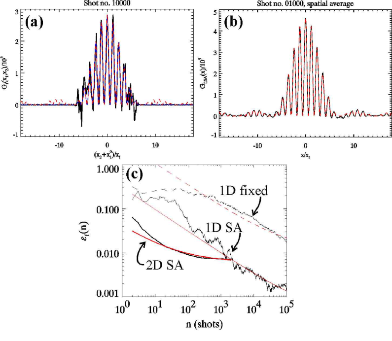
Fig. 3: Reconstructing the diffraction pattern using the f-f setup in the reference arm. (a) shows the correlation from a fixed $x_{1}$ after averaging over 10000 shots while (b) shows the correlation using the spatial averaging technique and averaging over 1000 shots. In (a) and (b) black curves are numerics, while dashed red curves are $\tilde{T}_{\rm obj}$. In (a) the blue curve is the analytically calculated correlation in the SPWPA in arbitrary units [Eq. (6) including integration over time, as shown in Eq. (5)]. (c) shows $\varepsilon(n)$ from Eq. (12) in a double-logarithmic plot using the spatial averaging technique (full) and a fixed detector (dashed), while the red curves are fits to Eq. (13). Double slit parameters: aperture 14 $\mu$m (5 pixels) and aperture center distance 87 $\mu$m (30 pixels). [Movie sizes: (a) 1 MB and (b) 933 KB].

Let us show quantitatively how the object diffraction pattern is reconstructed by using a double slit as an object in the setup of Fig. 1(a). The correlations as calculated in 1D both with and without the spatial average are presented in Fig. 3(a)-(b). The correlation without spatial average in (a) clearly suffers from a limited bandwidth, and from the animation a slow convergence rate is evident. In contrast, the correlation with spatial average in (b) is able to reproduce the entire spectrum of the diffraction pattern and after much fewer repeated pump shots. To check the convergence rate, we have calculated the root-mean-squared error of the correlation $G_{\rm{f}}^{n}$ (after averaging over $n$ number of shots) relative to the analytically calculated correlation $G_{\rm{f}}$. $G_{\rm{f}}$ was calculated by using semi-analytical methods including the analytical SPWPA gain as well as integrating over time [see Eq. (5)]. The error is then evaluated as

$$\varepsilon_{\rm f}(n)=\left(\Sigma_{{\bf x}}|G_{\rm{f}}^{n}({\bf x})-G_{\rm{f}}({\bf x})|^{2}\right)^{1/2}$$ (12)

where at each shot the maximum of $G_{\rm{f}}^{n}$ is rescaled to the maximum of $G_{\rm{f}}$. Figure 3(c) shows $\varepsilon(n)$ and clearly the fixed detector case (dashed) converges much slower than the spatial average (full). The red curves are fits to the function

$$\varepsilon_{\rm fit}(n)=(d_{0}n)^{-1/2}+d_{1}$$ (13)

with $n$ being the number of shots. The factor $d_{0}$ has the dimension shot^-1 and the ratio between $d_{0}$’s obtained using the spatial average and using fixed detector should then give an indication of the increased convergence rate. From the fits of Fig. 3(c), $d_{0}^{{\rm SA},\rm 1D}/d_{0}^{\rm fixed,\rm 1D}\simeq 125$, which corresponds well to the value $\rho_{\rm SA}\simeq 10^{2}$ estimated in the previous section. The factor $d_{1}$ indicates the error remaining after convergence, but in this case the correlations are not converged sufficiently within the number of shots shown. Now, according to what was predicted in Eq. (8), using the spatial average in 2D should benefit with a factor of $\rho_{\rm SA}$ in convergence speedup compared to using the spatial average in the 1D case (due to the extra dimension to average over). In Fig. 3(c) the result of such a 2D simulation is also shown, and the improved convergence rate of the 2D simulation is evident: from the fits $d_{0}^{{\rm SA},\rm 2D}/d_{0}^{{\rm SA},\rm 1D}\simeq 73$, again corresponding well to the predicted estimate of $\rho_{\rm SA}\simeq 10^{2}$. A minor problem in this comparison is that the 2D results saturate very quickly to a rather high error level of 1%, while the 1D results go as low as 0.1%. This difference turned out to be caused by the Gaussian shape of the pump field and the object extension; the object is very localized in the $x$ direction and therefore we get a low error rate in the 1D case. However, in the 2D case the object is quite extended in the $y$ direction and the average error reported in the $\varepsilon$ value is therefore higher. This quick saturation in 2D gave some numerical problems in fitting well the data to Eq. (13), so the $d_{0}$ value obtained should be taken cautiously. However, there is no doubt about the main point: going from 1D to 2D the spatial averaging technique speeds further up.

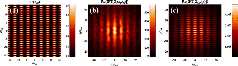
Fig. 4: Reconstructing the diffraction pattern of the object shown in (a) which has spatial Fourier components both inside and outside the PDC bandwidth. The real part of the inverse Fourier transform of the reconstructed diffraction pattern using the f-f setup is shown with (b) fixed ${\bf x}_{1}$ and (c) using the spatial averaging technique. $35000$ shots were used.

Let us show an example where the reconstructed diffraction pattern using the f-f setup leads to completely different results depending on whether the spatial average is applied or not. The object is shown in Fig. 4(a) and is a 2D mask $T_{\rm obj}({\bf x})=[1+\cos(xq_{0})][1+\cos(3yq_{0})]/4$ (consisting of 4 main sidebands, 2 located at ${\bf q}/q_{0}=\pm{\bf e}_{x}$ and 2 located at ${\bf q}/q_{0}=\pm 3{\bf e}_{y}$). We have chosen the peaks in the $y$-direction so they lie outside the imaging bandwidth of the source, while the peaks in the $x$-direction lie inside the bandwidth. In the numerics the diffraction pattern was reconstructed from the correlation with ${\bf x}_{1}$ fixed as well as employing the spatial averaging technique. Instead of showing these data, we have in Fig. 4(b) and (c) shown the results after taking the inverse Fourier transform (IFT) of the reconstructed diffraction patterns. In this way we can reconstruct to some extend the nature of the near field mask (some phase information is lost, obviously, but in this simple case the lost phase information is not so important). Figure 4(b) shows ${\rm Re}({\rm IFT}[G_{\rm f}({\bf x}_{1},{\bf x}_{2})])$, i.e. without spatial average, and only the roll pattern in the $x$-direction is reproduced. Instead, the correct object is reproduced by the result ${\rm Re}({\rm IFT}[G_{{\rm f},{\rm SA}}({\bf x})])$ from using the spatial average, as shown in Fig. 4(c).

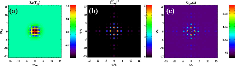
Fig. 5: The reconstructed diffraction pattern of a phase object with the spatial averaging technique. (a) shows ${\rm Re}(T_{\rm obj})$ consisting of $4\times 4$ square holes (with the value $T_{\rm obj}=-1$ inside and $T_{\rm obj}=+1$ outside the holes) modulated by a Gaussian. (b) analytical $|\tilde{T}_{\rm obj}|^{2}$. (c) $G_{{\rm f},{\rm SA}}$ after 2000 shots.

The imaging system with the reference arm set in the f-f setup is able to reconstruct the diffraction pattern of a pure phase object, both with and without the spatial averaging technique applied (the latter was already demonstrated in Ref. [10]). The chosen object [see Fig. 5(a)] was a pure phase object modulated by a Gaussian as to avoid a cosmetically disturbing DC peak [the analytical Fourier transform is shown in Fig. 5(b)]. An imaging scheme that is unable to reconstruct phase information would therefore only show the Fourier transform of the Gaussian which is another Gaussian. Figure 5(c) shows the result of a numerical simulation in 2D where the spatial averaging technique was used, and it closely follows the analytical diffraction pattern of the object in Fig. 5(b) confirming that phase information is preserved.

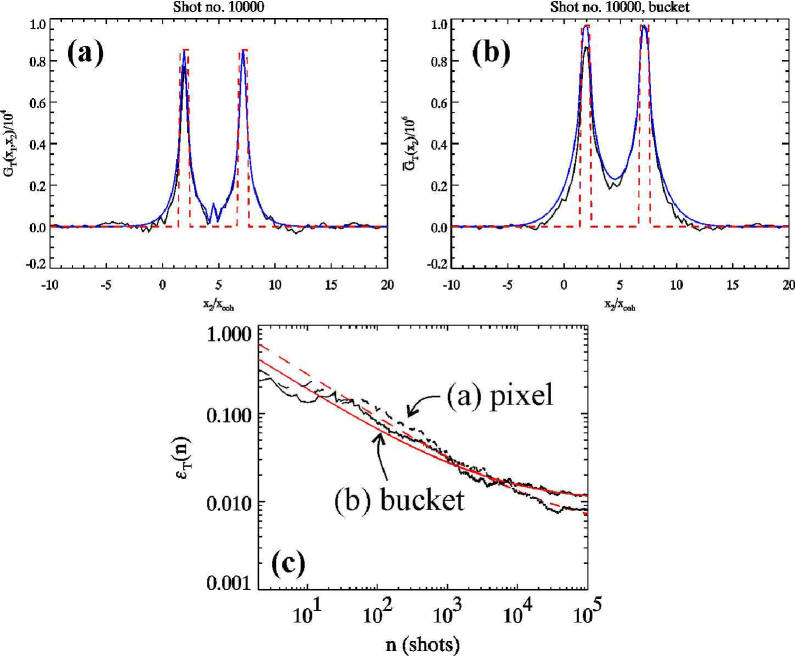
Fig. 6: The reconstructed image using the telescope setup with (a) $D_{1}$ a pixel-like detector and (b) $D_{1}$ a bucket detector. The black curves are numerics, the dashed red curves are $T_{\rm obj}$, while the blue curves are the analytically calculated correlations in the SPWPA in arbitrary units [Eqs. (14) and (15)]. (c) shows $\varepsilon_{\rm T}(n)$ (full: bucket detector and dashed: pixel detector), and the red curves are fits to Eq. (13). The same parameters and notation as in Fig. 3. [Movie sizes: (a) 748 KB and (b) 1.25 MB].

The image of the object can be reconstructed by merely changing the setup in the reference arm to the telescope setup [see Fig. 1(b)]. Figure 6 compares using (a) a pixel-like detector and (b) a bucket detector in the test arm for this case. In both cases the double slit is reproduced, albeit with the characteristic blurring of the sharp contours of the double slit apertures because of the finite resolution. In fact, the aperture size of the double slit (14 $\mu$m) is on the limit of the system’s resolution $x_{\mathrm{coh}}\simeq 16~{}\mu$m. The convergence rates as observed in the animations seem identical, which is confirmed by the error plot on the right [showing the image version of (12), i.e. $\varepsilon_{\rm T}(n)=\left(\Sigma_{{\bf x}}|G_{\rm{T}}^{n}({\bf x})-G_{\rm{T}}({\bf x})|^{2}\right)^{1/2}$].

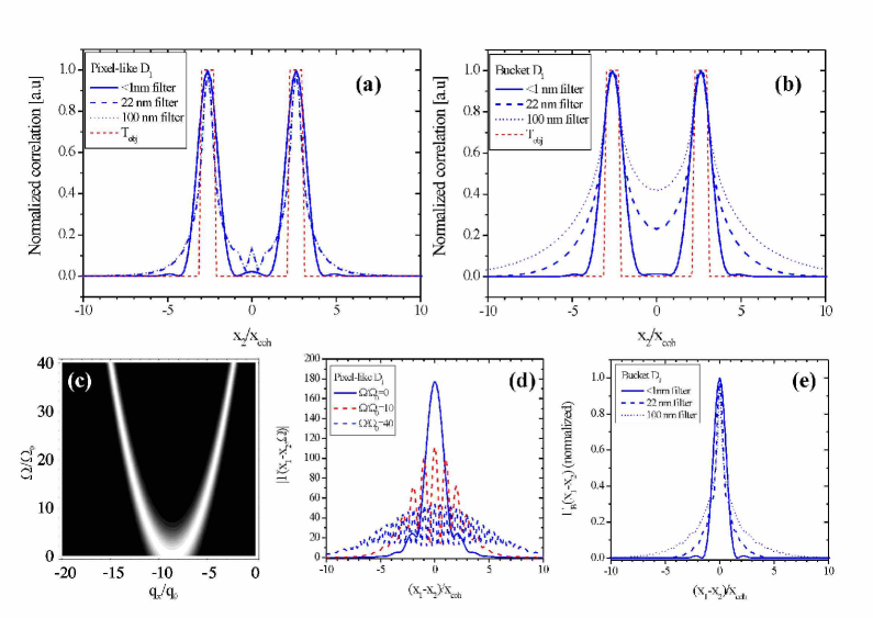
Fig. 7: The reconstructed image from semi-analytical calculations with (a) $D_{1}$ a pixel-like detector and (b) $D_{1}$ a bucket detector, using different interferential filters (different temporal bandwidths). The blue curves are semi-analytical calculations in the SPWPA in arbitrary units [Eqs. (14) and (15)]. (c) shows $|\gamma(q_{x},\Omega)|$ for the chosen PDC setup. (d) shows $|\Gamma({\bf x}_{1}-{\bf x}_{2},\Omega)|$ for different values of $\Omega$. (e) shows $\Gamma_{\rm B}({\bf x}_{1}-{\bf x}_{2})$ for different interferential filters.

From the semi-analytical calculations an interesting observation about the resolution abilities of the imaging scheme emerged when varying the interference filter after the PDC crystal, which filters a frequency range $[-\delta\Omega,\delta\Omega]$. In the case considered in the analytical section $\delta\Omega=0$, which in practice corresponds to a $<1$ nm interference filter. The numerics with time used $\delta\Omega=40\Omega_{0}$, i.e. a 22 nm filter. Figure 7(a) shows the case where $D_{1}$ is a pixel-like detector; the result remains more or less unchanged as the interference filter changes and no noticeable difference is observed between the 22 nm and 100 nm filters. In contrast, when $D_{1}$ is a bucket detector the result is much more sensitive; as shown in Fig. 7(b) the narrow interference filter gives the best resolution, while taking a broader filter gives a deteriorating resolution. The explanations for these different behaviours are found from considering the two explicit expressions for the correlations integrated over time. From Eq. (5) we namely find instead of Eqs. (9) and (11)

$$G_{\rm T}({\bf x}_{1},{\bf x}_{2})\propto\int{\rm d}\Omega\left|\int{\rm d}{\bf x}^{\,\prime}_{1}\Gamma({\bf x}^{\,\prime}_{1}-{\bf x}_{2},\Omega)T_{\rm obj}\left({\bf x}^{\,\prime}_{1}\right)e^{-i{\bf x}^{\,\prime}_{1}\cdot{\bf x}_{1}k/f}\right|^{2},\quad\text{ coherent (pixel-like~{}$D_{1}$)}$$ (14)

$$\bar{G}_{\rm T}({\bf x}_{2})\propto\int{\rm d}\Omega\int{\rm d}{\bf x}_{1}|\Gamma({\bf x}_{1}-{\bf x}_{2},\Omega)|^{2}|T_{\rm obj}\left({\bf x}^{\,\prime}_{1}\right)|^{2},\quad\text{ incoherent (bucket~{}$D_{1}$)}.$$ (15)

Thus, in the coherent case $\Gamma({\bf x}^{\,\prime}_{1}-{\bf x}_{2},\Omega)$ acts at each $\Omega$ as an imaging kernel, which is shown in Fig. 7(d) for different values of $\Omega$. As $\Omega$ increases $\Gamma({\bf x}^{\,\prime}_{1}-{\bf x}_{2},\Omega)$ becomes broader and the sidebands become pronounced. This can be understood by noting that Eq. (4) expresses $\Gamma({\bf x}^{\,\prime}_{1}-{\bf x}_{2},\Omega)$ as the inverse Fourier transform of $\gamma({\bf q},\Omega)$, which is shown in Fig. 7(c): as $\Omega$ increases $\gamma({\bf q},\Omega)$ becomes double-peaked, giving the sideband oscillations. All these contributions should then be added up as the integration in $\Omega$ is carried out. It is therefore important to notice that $\Gamma({\bf x}^{\,\prime}_{1}-{\bf x}_{2},\Omega)$ becomes weaker as $\Omega$ is increased. Therefore, despite the fact that the broader sidebands in $\Gamma({\bf x}^{\,\prime}_{1}-{\bf x}_{2},\Omega)$ imply a deteriorating resolution, the reduced peak value of $\Gamma({\bf x}^{\,\prime}_{1}-{\bf x}_{2},\Omega)$ implies that the end result is affected less and less as $\Omega$ is increased. Thus, the coherent nature of the imaging explains why the image does not change much as the bandwidth is increased in Fig. 7(a). In the bucket detector case the situation is completely different. Instead of having many contributions from different $\Omega$, the incoherence of the imaging system implies that the temporal integration defines a new imaging kernel as

$$\Gamma_{\rm B}({\bf x}_{1}-{\bf x}_{2})\equiv\int\frac{{\rm d}\Omega}{2\pi}|\Gamma({\bf x}_{1}-{\bf x}_{2},\Omega)|^{2}.$$ (16)

so $\bar{G}_{\rm T}({\bf x}_{2})\propto\int{\rm d}{\bf x}_{1}\Gamma_{\rm B}({\bf x}_{1}-{\bf x}_{2},\Omega)|T_{\rm obj}\left({\bf x}_{1}\right)|^{2}$. Thus, $\Gamma_{\rm B}({\bf x}_{1}-{\bf x}_{2})$ uniquely determines the resolution of the incoherent imaging system, and from Fig. 7(e) we see it becomes broader as the frequency bandwidth is increased, implying a decrease in resolution which is exactly what was seen in Fig. 7(b). We should stress that this result is a particular consequence of the PDC phase-matching conditions and does therefore not necessarily apply to ghost imaging schemes using other sources for the correlated beams.

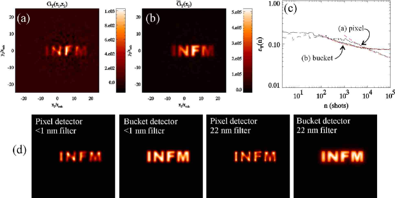
Fig. 8: The reconstructed near field of a mask with the letters “INFM” using the telescope setup. In the numerical simulations of (a) $D_{1}$ was a pixel-like detector, while in (b) $D_{1}$ was a bucket detector. (c) shows the convergence rate of the two cases (same notation as in Fig. 6.) $10^{5}$ shots were used, as well as a larger pump waist than usual (corresponding to $800~{}\mu$m). (d) shows semi-analytical calculations without time ($<1$ nm filter) and with time (22 nm filter).

In 2D the advantage of using the bucket detector for the image reconstruction becomes more obvious. As an example of a reasonably complicated object, we have in Fig. 8 reconstructed a mask with the letters “INFM”. The difference between the pixel-detector case (a) and the bucket detector case (b) is again related to coherent vs. incoherent imaging. The semi-analytical calculations in (d) in the SPWPA confirm this; whereas the pixel-detector result is suffering from a speckle-like effect [16], this effect is absent in the bucket-detector result. Note also the different results obtained from a narrow and a broad bandwidth filter, as discussed in the previous paragraph [the numerics in Fig. 8(a)-(b) are without time, so they should be compared to $<1$ nm filter results of Fig. 8(d)]. Finally, (c) shows $\varepsilon(n)$, and it is evident that the bucket-detector case (full lines) converges faster than the pixel-detector case (dashed lines); from the fits we obtain $d_{0}^{\rm bucket}/d_{0}^{\rm pixel}\simeq 20$. This speedup in convergence is a consequence of the bucket detector $D_{1}$ making a spatial average over the field at the test arm detection plane, and the magnitude of the speedup is therefore related to the number of independent modes recorded by $D_{1}$. In 1D this number is much smaller than in 2D which is why no significant speedup was observed in the 1D case (Fig. 6).

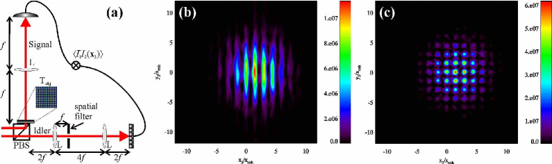
Fig. 9: Non-local filtering using the telescope setup with a bucket detector in the test arm. The setup (a) was as Fig. 1(b) but with a spatial filter inserted in the focal plane of the first lens in the reference arm. (b) shows the correlation using the filter, while (c) shows the correlation without filter. 15000 shots were used.

If filters are inserted in the reference arm the reconstructed object can be manipulated. As a simple example of this, using the telescope setup in the reference beam we have inserted a filter in the focal plane of the first lens [see Fig. 9(a)]. The object in the test arm was a square pattern $T_{\rm obj}({\bf x})=[1+\cos(3xq_{0}/2)][1+\cos(3yq_{0}/2)]/4$ (consisting of 4 main sidebands, 2 located at ${\bf q}/q_{0}=\pm\frac{3}{2}{\bf e}_{x}$ and 2 located at ${\bf q}/q_{0}=\pm\frac{3}{2}{\bf e}_{y}$.). Filtering in the $y$-direction we observe only rolls in the $x$-direction [Fig. 9(b)], while removing the filter the square pattern is seen in the correlations [Fig. 9(c)]. This shows that the image Fourier components can be manipulated non-locally.

4 Conclusion

The ghost imaging schemes rely on two spatially correlated beams. These are generated by a source with a limited spatial bandwidth in Fourier space, which determines the highest Fourier component in the diffraction pattern of the object that can be reproduced (i.e., the imaging bandwidth is limited). In turn, the resolution of the reconstructed image is limited by the characteristic near-field coherence length of the source.

In this paper we have through theory and numerics analyzed in detail a technique (already presented by us in [12] for a different imaging scheme) that improves the imaging bandwidth by implementing a spatial average over the test arm detector position. This technique makes the imaging bandwidth of the reconstructed diffraction pattern virtually infinite (apart from limitations arising from lenses and apertures), as well as making the correlations converge much faster. We showed that the speed-up of this convergence is related to the number of statistically independent modes inside the source bandwidth. When reconstructing the object image no benefits to the image resolution could be made by doing a spatial average. However, by merely using a bucket detector collecting all photons in the test arm, the imaging becomes incoherent. Whether coherent or incoherent imaging is advantageous depends obviously on the problem at hand [16], but we showed examples where the speckle problem of coherent imaging could be avoided using a bucket detector. On the other hand, when using a bucket detector it turned out to be important to use a narrow-band interference filter of the down-converted beams, otherwise a strong degrading in resolution was observed. Finally, we also showed that by inserting a filter in the focal plane of a lens in the reference arm, the reconstructed image could be non-locally filtered; the filter never interferes with the field containing the object information but through the correlations the image is filtered nonetheless.

We have in this paper chosen to focus on an imaging scheme using spatially entangled PDC beams. However, we should stress that practically all the results shown are general for any imaging system, quantum or classical, and are therefore relevant also for the important case when classical spatially correlated beams are created by splitting a thermal-like radiation on a beam splitter [10, 13]. In that case, e.g. the near-field correlation function (4) is instead governed by the second-order correlation of the thermal field [10], but the overall results of this paper remains the same. Thus, the spatial averaging technique may still be used to extend the bandwidth and speed up the convergence. In this connection it should be stressed that with thermal-like beams the reconstructed object image has exactly the same properties as when using PDC beams: it is coherent of one uses a pixel-like detector, while it becomes incoherent if a bucket detector is used.