Deterministic event-based simulation of quantum interference

Abstract

We propose and analyse simple deterministic algorithms that can be used to construct machines that have primitive learning capabilities. We demonstrate that locally connected networks of these machines can be used to perform blind classification on an event-by-event basis, without storing the information of the individual events. We also demonstrate that properly designed networks of these machines exhibit behavior that is usually only attributed to quantum systems. We present networks that simulate quantum interference on an event-by-event basis. In particular we show that by using simple geometry and the learning capabilities of the machines it becomes possible to simulate single-photon interference in a Mach-Zehnder interferometer. The interference pattern generated by the network of deterministic learning machines is in perfect agreement with the quantum theoretical result for the single-photon Mach-Zehnder interferometer. To illustrate that networks of these machines are indeed capable of simulating quantum interference we simulate, event-by-event, a setup involving two chained Mach-Zehnder interferometers. We show that also in this case the simulation results agree with quantum theory.

I Introduction

Computer simulation is widely regarded as complementary to theory and experiment LAND00 . At present there are only a few physical phenomena that cannot be simulated on a computer. One such exception is the double-slit experiment with single electrons, as carried out by Tonomura and his co-workers TONO98 . This experiment is carried out in such a way that at any given time, only one electron travels from the source to the detector PerfectExperiments . Only after a substantial (approximately 50000) amount of electrons have been detected an interference pattern emerges TONO98 . This interference pattern is described by quantum theory. We use the term “quantum theory” for the mathematical formalism that gives us a set of algorithms to compute the probability for observing a particular event HOME97 ; KAMP88 ; QuantumTheory . Of course, the quantum-mechanics textbook example FEYN65 ; BALL03 of a double-slit can be simulated on a computer by solving the time-dependent Schrödinger equation for a wave packet impinging on the double slit RAED96 ; QMvideo . Alternatively, in order to obtain the observed interference pattern we could simply use random numbers to generate events according to the probability distribution that is obtained by solving the time-independent Schrödinger equation. However, that is not what we mean when we say that the physical phenomenon cannot be simulated on a computer. The point is that it is not known how to simulate, event-by-event, the experimental observation that the interference pattern appears only after a considerable number of events have been recorded on the detector. Quantum theory does not describe the individual events, e.g. the arrival of a single electron at a particular position on the detection screen TONO98 ; HOME97 ; FEYN65 ; BALL03 . Reconciling the mathematical formalism (that does not describe single events) with the experimental fact that each observation yields a definite outcome is often referred to as the quantum measurement paradox and is the central, most fundamental problem in the foundation of quantum theory FEYN65 ; HOME97 ; PENR90 .

If computer simulation is indeed a third methodology to model physical phenomena it should be possible to simulate experiments such as the two-slit experiment on an event-by-event basis. In view of the fundamental problem alluded to above there is little hope that we can find a simulation algorithm within the framework of quantum theory. However, if we think of quantum theory as a set of algorithms to compute probability distributions there is nothing that prevents us from stepping outside the framework that quantum theory provides. Therefore we may formulate the physical processes in terms of events, messages, and algorithms that process these events and messages, and try to invent algorithms that simulate the physical processes. Obviously, to make progress along this line of thought, it makes sense not to tackle the double-slit experiment directly but to simplify the problem while retaining the fundamental problem that we aim to solve.

The main objective of the research reported in this paper is to answer the question: “Can we simulate the single-photon beam splitter and Mach-Zehnder interferometer experiments of Grangier et al. GRAN86 on an event-by-event basis?”. These experiments display the same fundamental problem as the single-electron double-slit experiments but are significantly easier to describe in terms of algorithms. The main results of our research are that we can give an affirmative answer to the above question by using algorithms that have a primitive form of learning capability and that the simulation approach that we propose can be used to simulate other quantum systems (including the double-slit experiment) as well.

In Section II we introduce the basic concepts for constructing event-based, deterministic learning machines (DLMs). An essential property of these machines is that they process input event after input event and do not store information about individual events. A DLM can discover relations between input events (if there are any) and responds by sending its acquired knowledge in the form of another event (carrying a message) through one of its output channels. By connecting an output channel to the input channel of another DLM we can build networks of DLMs. As the input of a network receives an event, the corresponding message is routed through the network while it is being processed and eventually a message appears at one of the outputs. At any given time during the processing, there is only one input-output connection in the network that is actually carrying a message. The DLMs process the messages in a sequential manner and communicate with each other by message passing. There is no other form of communication between different DLMs. Although networks of DLMs can be viewed as networks that are capable of unsupervised learning, there have very little in common with neural networks HAYK99 . The first DLM described in Section II is equivalent to a standard linear adaptive filter HAYK86 but the DLMs that we actually use for our applications do not fall into this class of algorithms.

In Section III we generalize the ideas of Section II and construct a DLM which groups $K$-dimensional data in two classes on an event-by-event basis, i.e., without using memory to store the whole data set. We demonstrate that this DLM is capable of detecting time-dependent trends in the data and performs blind classification. This example shows that DLMs can be used to solve problems that have no relation to quantum physics.

In Section IV we show how to construct DLM-networks that generate output patterns that are usually thought of as being of quantum mechanical origin. We first build a DLM-network that simulates photons passing through a polarizer and show that quantum theory describes the output of this deterministic, event-based network. Then we describe a DLM-network that simulates a beam splitter and use this network to build a Mach-Zehnder interferometer and two chained Mach-Zehnder interferometers. We demonstrate that quantum theory also describes the behavior of these networks.

Quantum theory gives us a recipe to compute the frequency of events but does not predict the order in which the events will be observed BALL03 ; HOME97 . In genuine experiments the detection of events appears to be random GRAN86 ; TONO98 , in a sense which, as far as we know, has not been studied systematically. In our simulation approach, this apparent randomness can be accounted for by a marginal modification of the DLMs, as explained in Section V. This modification does not change the deterministic character of the learning process. It merely randomizes the order in which the DLMs activate their output channels.

A summary and outlook is given in Section VI.

II Deterministic learning machines

II.1 Learning points on the real axis

We consider a machine that has one input and two output channels labeled by $\pm 1$ (see Fig. 1). The internal state of the machine after processing the $n$-th input event ($n=0,1,\ldots$) is uniquely defined by the real variable $x_{n}$. At the next event $n+1$ the machine receives as input a real number $y_{n+1}$. For simplicity, but without loss of generality, we assume that $y_{n+1}\in[-1,1]$. The machine responds by sending a message containing $y_{n+1}$ through one of the two output channels $\Delta_{n+1}=\pm 1$. The machine selects the output channel $\Delta_{n+1}=+1$ or $\Delta_{n+1}=-1$ by minimizing the cost function $C(\Delta_{n+1})$ defined by

$$C(\Delta_{n+1})=|y_{n+1}-x_{n}-(1-\alpha)\Delta_{n+1}|y_{n+1}-x_{n}||,$$ (1)

updates its internal state according to the rule

$$x_{n+1}=x_{n}+(1-\alpha)\Delta_{n+1}|y_{n+1}-x_{n}|,$$ (2)

and sends a message with the input value $y_{n+1}$ on the selected output channel $\Delta_{n+1}$. The parameter $0<\alpha<1$ that enters Eqs. (1) and (2) controls the decision process. For simplicity we assume that $\alpha$ is fixed during the operation of the machine.

It is easy to see that $\Delta_{n+1}=+1$ if $x_{n}\leq y_{n+1}$ and $\Delta_{n+1}=-1$ if $x_{n}>y_{n+1}$. Thus, for this particular machine we have

$$\Delta_{n+1}=\frac{y_{n+1}-x_{n}}{|y_{n+1}-x_{n}|}.$$ (3)

Hence the update rule Eq. (2) can be written as the familiar recursion

$$x_{n+1}=\alpha x_{n}+(1-\alpha)y_{n+1}.$$ (4)

The solution of Eq. (4) reads

$$x_{n}=\alpha^{n}x_{0}+(1-\alpha)\sum_{i=0}^{n-1}\alpha^{n-1-i}y_{i+1},$$ (5)

where $x_{0}$ denotes the initial value of the internal variable.

As an illustration of how this machine learns, we consider the most simple example where $y_{n+1}=y$ for all $n\geq 0$. Then from Eq. (5) we find that

$$x_{n}=\alpha^{n}x_{0}+(1-\alpha^{n})y.$$ (6)

As $0<\alpha<1$, we conclude that $\lim_{n\rightarrow\infty}x_{n}=y$. Thus the machine “learns” the value of the input variable $y$. From Eq. (4) it follows that $x_{n}\leq y$ ($x_{n}\geq y$) implies $x_{n+1}\leq y$ ($x_{n+1}\geq y$). Hence $x_{n}$ approaches $y$ monotonically (and $\Delta_{n}$ is the same for all $n$). Therefore, if $y_{n}=y$, the machine always sends the value of $y_{n}$ through the same output channel.

Figure 1: Left: Schematic representation of the machine that responds to the input $y_{n+1}$ by passing the input to one of the two output channels $\Delta_{n+1}=\pm 1$. The value of $\Delta_{n+1}$ depends on the current state of the machine, encoded in the variable $x_{n}$, the input $y_{n+1}$, and the update rule Eq. (2) in which $\alpha$ appears as a control parameter. Right: Evolution of the internal variable $x_{n}$ as a function of the number of events $n$. Solid line: $y_{n+1}=-0.5$ for $n=1,\ldots,1000$ and $y_{n+1}=0.5$ for $n=1001,\ldots,2000$; Dashed line: Random sequence of $y_{n+1}=\pm 0.5$.

A distinct feature of this machine is its ability to adapt to changes in the input pattern. We illustrate this important property by two examples. Let $y_{n}=-0.5$ for $1\leq n\leq 1000$ and $y_{n}=0.5$ for $1000<n\leq 2000$. During the first 1000 events the machine will learn $-0.5$. After 1000 events only $0.5$ is being presented as input. Then, the machine “forgets” $-0.5$ and learns $0.5$ as shown in the right panel of Fig. 1. In this simulation $\alpha=0.99$. Alternatively, if $y_{n}$ is a random sequence of $\pm 0.5$ (each with the same probability) the machine has to learn $-0.5$ and $0.5$ simultaneously. Because of this it cannot “forget” and it ends up oscillating around the mean of the input values (zero in this example) as illustrated in the right panel of Fig. 1. Let us now assume that our machine has reached this oscillating state. All input events $y_{n}=0.5$ give $\Delta_{n}=+1$ and hence the machine sends $0.5$ over the $+1$ channel. A second machine attached to this channel only receives $0.5$ events and will learn $0.5$. This suggests that a network of these machines can be used as an adaptive classifier.

Figure 2: Left: Diagram of the three-level machine that adaptively classifies the input data $y_{n+1}$. Right: Evolution of the internal variables $x_{n}$ of the machines as a function of the number of events $n$. The machine number is used to label the corresponding line. Top right: First three machines; Bottom right: Third-level machines.

Consider the network of three layers of machines shown in the left panel of Fig. 2. Each machine in the network learns the average of the numbers it receives at its input channel and sends the numbers which are smaller (larger or equal) than the number it learned to the -1 (+1) output channel. In our numerical experiments we set $\alpha=0.99$. We start with 5000 events of random numbers $y_{n+1}\in\{-0.75,-0.25,0.25,0.75\}$, each occurring with equal probability. Machine 1 learns the average (zero in this example) and sends the negative (positive) $y_{n+1}$ over the $-1$ ($+1$) channel to the input of machine 2 (3). Machine 2 (3) learns -0.50 (0.50), as shown in the top right panel of Fig. 2, and sends -0.75 (0.25) over its -1 output channel and -0.25 (0.75) over its +1 output channel. Machines 4 to 7 learn -0.75,-0.25,0.25 and 0.75, respectively, as shown in the bottom right panel of Fig. 2. Each of these machines forwards the received input on its +1 (-1) output channel if the initial value of its internal variable is smaller (larger) than the received input value. Let us now assume that after 5000 events the input data set changes to $y_{n+1}\in\{-0.75,-0.25,0.25,0.50\}$. As can be seen from the right panel of Fig. 2, machines 1, 3 and 7 “forget” the number they learned and replace it by -0.0625, 0.375 and 0.50, respectively. All other machines are unaffected because they never get 0.50 as input. After another 5000 events we change the set of input values once more, this time to $y_{n+1}\in\{-0.60,-0.75,-0.25,0.25,0.50\}$, i.e., we add one element. Now, machine 1 learns -0.17, machine 2 learns -0.53 and the internal state of machine 3 remains unchanged. Machine 4 can now receive two numbers on its input channel, namely -0.75 and -0.60. As a consequence, machine 4 learns -0.675, i.e., the average of the two possible input numbers. Machine 4 puts -0.60 on its +1 output channel and -0.75 on its -1 output channel. In order for the network to learn all the numbers of the input set, we would have to attach one extra machine to each output channel of machine 4.

Figure 3: Left: Time evolution of the internal variable $x_{n}$ of the machine defined by Eqs. (7) and (8). The input events are $y=-0.25$, $\alpha=0.99$, and the initial value $x_{0}=0$. For $n>30$ the internal variable $x_{n}$ oscillates about $y$. For $n>500$ the sequence of increments ($\Delta_{n+1}=+1$) and decrements ($\Delta_{n+1}=-1$) of $x_{n}$ repeats itself after 8 events (data not shown). Lines are guides to the eyes. Right: The number of increments of the internal variable ($\Delta_{n+1}=+1$) divided by the total number of events as a function of the value of the input variable $y$. Bullets: Each data point is obtained from a simulation of 1000 events with a fixed, randomly chosen value of $-1<y<1$, using the last 500 events to count the number of $\Delta_{n+1}=+1$ events. Solid line: $(1+y)/2$.

II.2 Learning points on a finite interval

For the machine defined by Eqs. (1) and (2), formulating the operation of the machine through the minimization of the difference between the input and internal variable may seem a little superfluous and indeed, for this particular machine it is. However, this formulation is a convenient starting point for defining machines that can perform more intricate tasks. For instance, let us make an innocent looking change to the update rule Eq. (2) by writing

$$x_{n+1}=\alpha x_{n}+(1-\alpha)\Delta_{n+1},$$ (7)

and replace the cost function Eq. (1) by the corresponding expression

$$C(\Delta_{n+1})=|y_{n+1}-\alpha x_{n}-(1-\alpha)\Delta_{n+1}|.$$ (8)

For $\Delta_{n+1}=+1$ we have $x_{n+1}=1-\alpha(1-x_{n})$ and for $\Delta_{n+1}=-1$ we have $x_{n+1}=-1+\alpha(1+x_{n})$. Therefore, if $0<\alpha<1$ and $|x_{0}|\leq 1$, the internal variable will always be in the range $[-1,1]$. At each event the internal variable either increases by $(1-\alpha)(1-x_{n})$ (if $\Delta_{n+1}=+1$) or decreases by $(1-\alpha)(1+x_{n})$ (if $\Delta_{n+1}=-1$). In both cases this change is always nonzero, except if $x_{n}=\pm 1$ which can only occur if $y_{n+1}=\pm 1$. The ratio of the step sizes is $(1-x_{n})/(1+x_{n})$.

The machine defined by Eqs. (7) and (8) behaves differently from the machine defined by Eqs. (1) and (2). To see this, it is instructive to consider the case $0\leq y_{n+1}=y<1$ for all $n\geq 0$ (the case $-1<y_{n+1}=y<0$ can be treated in the same manner). For concreteness we assume that $-1<x_{0}<y$. At the first event, minimization of Eq. (8) yields $\Delta_{1}=+1$ and $x_{1}=1+\alpha(x_{0}-1)$. In other words, the internal variable $x$ moves towards $y$. As long as $x_{n}<y$, the machine selects $\Delta_{n+1}=+1$, always increasing its internal variable $x_{n}$. For some some $n\geq 1$ we must have $x_{n}>y$. Then, making another move in the positive $x$-direction allows for two different decisions. If the error that results is larger than the error that is obtained by moving in the negative direction the machine decides to set $\Delta_{n+1}=-1$. Otherwise it makes another move in the positive $x$-direction ($\Delta_{n+1}=+1$). In any case, for some $n>1$ the machine will select $\Delta_{n+1}=-1$. Note that when this happens, we must have $x_{n+1}<y$ and $\Delta_{n+2}=+1$. This implies that after this $n$-th event (that we denote by $n_{0}$) the internal variable will oscillate (forever) around the input value $y$. This process is illustrated in Fig. 3 (left).

For $m>n_{0}$ we have $|x_{m+1}-y|\leq(1-\alpha)\max(1-y,1+y)$. Thus, if $0<1-\alpha\ll 1$, the amplitude of the oscillations is small. The machine “learns” the input value $y$ and the ratio of the increments to decrements is $(1+x_{m+1})/(1-x_{m+1})\approx(1+y)/(1-y)$. In this stationary regime of oscillating behavior, the number of times the machine actives the +1 (-1) channel is given by $(1+y)/2$ ($(1-y)/2$). The simulation results shown in Fig. 3 (right) confirm the correctness of this analysis. For a fixed (unknown) value of the input variable, the rate at which the machine defined by the rules Eqs. (7) and (8) activates one of its output channels is determined by the value of its internal variable. Therefore, this rate reflects the value that the machine has learned by processing the input events. Depending on the application, the message that is sent through the active output channel can contain $x_{n+1}$ or the input value $y_{n+1}$ (there is nothing else that can be send). Obviously we can make the learning process more precise by increasing $\alpha<1$. Of course, a larger value of $\alpha$ also results in slower learning: In general it will take more events for the internal variable to reach the value where it starts to oscillate.

II.3 Learning points on a circle

In going from the first to the second example of Section II we changed the update rule such that the variable $x_{n}$ is constrained to lie in the interval $[-1,1]$. We now consider the two-dimensional analogue of the machines described in Section II.2 for which the internal vector $(x_{1,n},x_{2,n})$ and input vector $(y_{1,n+1},y_{2,n+1})$ represent points on a circle. This machine receives as input a sequence of angles $\phi_{n+1}$ defined by

$$\cos\phi_{n+1} = \frac{y_{1,n+1}}{\sqrt{y_{1,n+1}^{2}+y_{2,n+1}^{2}}},$$

$$\sin\phi_{n+1} = \frac{y_{2,n+1}}{\sqrt{y_{1,n+1}^{2}+y_{2,n+1}^{2}}},$$ (9)

and responds by activating one of the two output channels.

For all $n>0$, the update rules are defined by

$$x_{1,n+1} = \alpha x_{1,n}+\beta\Theta_{n+1},$$

$$x_{2,n+1} = \alpha x_{2,n}+\beta(1-\Theta_{n+1}),$$ (10)

where $\Theta_{n+1}=0,1$ and $0<\alpha<1$. In order that the internal vector ${\bf x}_{n+1}=(x_{1,n+1},x_{2,n+1})$ stays on the unit circle we must have

$$\beta=-\alpha[x_{1,n}\Theta_{n+1}+x_{2,n}(1-\Theta_{n+1})]\pm\sqrt{1-\alpha^{2}+\alpha^{2}[x_{1,n}^{2}\Theta_{n+1}+x_{2,n}^{2}(1-\Theta_{n+1})]}.$$ (11)

Substitution of Eq. (11) in Eq. (10) gives us four different rules:

$$x_{2,n+1} = s\sqrt{1+\alpha^{2}(x_{2,n}^{2}-1)}\quad,\quad x_{1,n+1}=\alpha x_{1,n}\quad\hbox{if }\Theta_{n+1}=0,$$

$$x_{1,n+1} = s\sqrt{1+\alpha^{2}(x_{1,n}^{2}-1)}\quad,\quad x_{2,n+1}=\alpha x_{2,n}\quad\hbox{if }\Theta_{n+1}=1,$$ (12)

where $s=\pm 1$ takes care of the fact that for each choice of $\Theta_{n+1}$, the machine has to decide between two quadrants. The cost function is defined by

$$C=-(x_{1,n+1}y_{1,n+1}+x_{2,n+1}y_{2,n+1}).$$ (13)

Obviously, the cost function Eq. (13) is nothing but the inner product of the vectors ${\bf x}_{n+1}$ and ${\bf y}_{n+1}$. The new internal state itself is determined by calculating the cost Eq. (13) for each of the four candidate update rules listed in Eq. (12) and selecting the rule that yields the minimum cost. Note that the minimum of the cost function Eq. (13) does not depend on the length of the vector of input variables $(y_{1,n+1},y_{2,n+1})$. From Eq. (12) it follows that if $\Theta_{n+1}=0$. the value of $x_{1,n+1}$ is obtained by rescaling of $x_{1,n}$ and $x_{2,n+1}$ is adjusted such that $x_{1,n+1}^{2}+x_{2,n+1}^{2}=1$. For $\Theta_{n+1}=1$ we interchange the role of the first and second element of ${\bf x}_{n+1}$.

Figure 4: Left: Time evolution of the angle representing the internal vector ${\bf x}_{n}$ of the machine defined by Eqs. (12) and (13). The input events are vectors ${\bf y}_{n+1}=(\cos 30^{\circ},\sin 30^{\circ})$. The direction of the initial vector ${\bf x}_{0}$ is chosen at random. In this simulation $\alpha=0.99$. For $n>60$ the ratio of the number of increments ($\Theta_{n+1}=0$) to decrements ($\Theta_{n+1}=1$) is 1/3, which is $(\sin 30^{\circ}/\cos 30^{\circ})^{2}$. Data for $n<20$ has been omitted to show the oscillating behavior more clearly. Lines are guides to the eyes. Right: The number of ($\Theta_{n+1}=1$) events divided by the total number of events as a function of the value of the input variable $\phi$. Bullets: Each data point is obtained from a simulation of 1000 events with a fixed, randomly chosen value of $0\leq\phi<360^{\circ}$, using the last 500 events to count the number of ($\Theta_{n+1}=1$) events. Solid line: $\cos^{2}\phi$.

In general the behavior of the machine defined by rules Eqs. (12) and (13) is difficult to analyze without the use of a computer. However, for a fixed input vector ${\bf y}_{n+1}={\bf y}$ it is clear what the machine will try to do: It will minimize the cost Eq. (13) by rotating its internal vector ${\bf x}_{n+1}$ to bring it as close as possible to ${\bf y}$. However, ${\bf x}_{n+1}$ will not converge to a limiting value but instead it will keep oscillating about the input value ${\bf y}$. An example of a simulation is given in Fig. 4 (left). For a fixed input vector ${\bf y}_{n+1}={\bf y}$ the machine reaches a stationary state in which its internal vector oscillates about ${\bf y}$. In this stationary state the output signal consists of a finite sequence of ones and zeros. The machine repeats this sequence over and over again. Obviously, the whole process is deterministic. The details of the approach to the stationary state depend on the initial value of the internal vector ${\bf x}_{0}$, but the stationary state itself does not.

These observations are of much more general nature than the example given in Fig. 4 (left) suggests. In fact, as the applications discussed below amply illustrate, the stationary-state analysis is a very useful tool to predict the behavior of the machines. Assuming that $0<1-\alpha\ll 1$ and that we have reached the stationary regime in which the internal vector performs small oscillations about $(\cos\phi,\sin\phi)$, a simple calculation shows that

$$\delta\phi_{0} = \phi_{1,n+1}-\phi_{1,n}\approx\frac{1-\alpha^{2}}{2}\frac{\cos\phi}{\sin\phi}\quad\hbox{if }\Theta_{n+1}=0,$$

$$\delta\phi_{1} = \phi_{1,n+1}-\phi_{1,n}\approx\frac{\alpha^{2}-1}{2}\frac{\sin\phi}{\cos\phi}\quad\hbox{if }\Theta_{n+1}=1.$$ (14)

In the stationary regime, we have $N_{0}\delta\phi_{0}\approx N_{1}\delta\phi_{1}$ where $N_{0}$ ($N_{1}$) is the number of $\Theta_{n+1}=0$ ($\Theta_{n+1}=1$) events. From Eq. (14) it then follows immediately that $N_{0}/(N_{0}+N_{1})\approx\sin^{2}\phi$ and $N_{1}/(N_{0}+N_{1})\approx\cos^{2}\phi$. The results of this analysis are in excellent agreement with the simulation results shown in Fig. 4 (right).

The conventional approach to regard the variables $\Theta_{n+1}$ as input is fundamentally different from the approach adopted in this paper. This can be seen by reformulating the update rules in terms of difference equations and to assume that the $\Theta_{n+1}=0,1$ are independent, uniform random variables with mean $\Theta=\langle\Theta_{n+1}\rangle$. The four rules Eq. (12) can be written as

$$x_{1,n+1}^{2} = \alpha^{2}x_{1,n}^{2}+(1-\alpha^{2})\Theta_{n+1},$$

$$x_{2,n+1}^{2} = \alpha^{2}x_{2,n}^{2}+(1-\alpha^{2})(1-\Theta_{n+1}).$$ (15)

Formally Eq. (15) has the same structure as Eq. (4). Averaging over many realizations of $\{\Theta_{n+1}=0,1\}$ and taking the limit $n\rightarrow\infty$ we obtain

$$\langle x_{1}^{2}\rangle = \lim_{n\rightarrow\infty}\langle x_{1,n+1}^{2}\rangle=\Theta,$$

$$\langle x_{2}^{2}\rangle = \lim_{n\rightarrow\infty}\langle x_{2,n+1}^{2}\rangle=1-\Theta.$$ (16)

In other words, a machine that operates according to the rules Eq. (12) and receives as input the random sequence $\Theta_{n+1}$ will (on average) approach a state in which the direction of its internal vector gives us an estimate of the $\Theta=\langle\Theta_{n+1}=0,1\rangle$. In contrast, a machine that minimizes the cost Eq. (13) and updates its internal state according to Eq. (12) responds on either output channel $\Theta_{n+1}=0$ or output channel $\Theta_{n+1}=1$, with a frequency that is directly related to the difference between the current input angle and the angle defined by the internal vector.

II.4 Learning points on a $K$-dimensional hypersphere

Consider a sequence of events, characterized by vectors ${\bf y}_{n+1}=(y_{1,n+1},y_{2,n+1},\ldots,y_{K,n+1})$ for $n>0$. The vector ${\bf y}_{n+1}$ is the input for the machine. The internal state of the machine is described by a $K$-dimensional unit vector ${\bf x}_{n}=(x_{1,n},x_{2,n},\ldots,x_{K,n})$. We define the $2K$ candidate update rules $\{j=1,\ldots,K;s_{j}=\pm 1\}$ by

$$x_{i,n+1} = s_{j}\sqrt{1+\alpha^{2}(x_{i,n}^{2}-1)}\quad\hbox{if}\quad i=j,$$

$$x_{i,n+1} = \alpha x_{i,n}\quad\hbox{if}\quad i\not=j.$$ (17)

Note that ${\bf x}^{T}_{n}{\bf x}^{\phantom{T}}_{n}=1$ implies ${\bf x}^{T}_{n+1}{\bf x}^{\phantom{T}}_{n+1}=1$ for each of the $2K$ update rules. The machine responds to the input ${\bf y}_{n+1}$ by selecting from the $2K$ possible rules in Eq. (17), the update rule that minimizes the cost

$$C=-{\bf x}^{T}_{n+1}{\bf y}^{\phantom{T}}_{n+1},$$ (18)

and by sending a message containing ${\bf y}_{n+1}$ (or, depending on the application, ${\bf x}_{n+1}$) on one of its output channels. Note that the minimum of the cost function Eq. (18) does not depend on the length of the vectors ${\bf x}_{n+1}$ or ${\bf y}_{n+1}$. Disregarding the variables $s_{j}$ that merely serve to determine the sign of $x_{i,n+1}$ there are $K$ rules. Hence there can be as many as $K$ output channels. However, depending on the application, it may be expedient to reduce the number of output channels by arranging them in groups.

II.5 Communication between events

The machines analyzed in the previous subsections have one input channel that receives input and two output channels, only one of which sends out data (a message) at a particular event. An obvious generalization is to construct machines that accept, at a given instance, input from one out of two different sources. This is absolutely necessary if we want to build machines in which events can communicate or, in physical terms, interact with each other. We now demonstrate that the machines that we introduced above already have the capability to let events interact with each other. Therefore we do not need to add a new feature or rule to the machines.

Consider a machine that has two input channels 0 and 1 and an internal vector ${\bf x}_{n}$ with $K=4$ components. At the $n+1$-th event, either input channel 0 receives the two-component vector ${\bf y}_{n+1}=(y_{1,n+1},y_{2,n+1})$ or input channel 1 receives the two-component vector ${\bf y}_{n+1}=(y_{3,n+1},y_{4,n+1})$.

In the former case the machine transforms this input into the input vector ${\bf\hat{y}}_{n+1}=(y_{1,n+1},y_{2,n+1},x_{3,n},x_{4,n})$ of four elements by using the current internal vector as a source for the missing elements. Similarly, in the latter case the input vector becomes ${\bf\hat{y}}_{n+1}=(x_{1,n},x_{2,n},y_{3,n+1},y_{4,n+1})$. Then the machine uses ${\bf\hat{y}}_{n+1}$ to determine the cost and selects the update rule according to the procedure described in Section II.4 (with ${\bf\hat{y}}_{n+1}$ replacing ${\bf y}_{n+1}$). This machine learns the two-dimensional vectors ${\bf y}_{n+1}=(y_{1,n+1},y_{2,n+1})$ and ${\bf y}_{n+1}=(y_{3,n+1},y_{4,n+1})$ separately, as if it consists of two separate, independent two-dimensional machines, with the additional crucial feature that the internal vector represents a point on a 4-dimensional unit sphere.

It is not difficult to imagine what this machine does in the case that it receives events on only one of the two input channels (say 0). Irrespective of the initial value of the internal vector ${\bf x}_{0}$, the machine will always select the update rule with $j=1,2$ (see Eq. (17)) and the two components $x_{3,n}$ and $x_{4,n}$ will vanish exponentially fast with increasing $n$ (recall that $0<\alpha<1$). Thus, after a few events the internal state of the machine indicates that the machine receives events on only one channel.

If the machine receives input on both channels (but never simultaneously), Eq. (17) implies that the machine only scales the two components of the internal state that it uses to provide the missing elements for building the input ${\bf\hat{y}}_{n+1}$. Therefore, in the stationary regime, the length of the two-dimensional vector $(x_{1,n},x_{2,n})$ ($(x_{3,n},x_{4,n})$) is proportional to the number of events on input channel 0 (1). Furthermore the number of $j=1,2$ ($j=3,4$) events is approximately equal to the number of events on input channel 0 (1). Although this may seem a very elementary form of communication, it is sufficient to construct machines that perform very complicated tasks.

II.6 Summary

The machines described above are simple deterministic machines that make decisions. The machine responds to the input event by choosing from all possible alternatives, the internal state that minimizes the error between the input and the internal state itself. Then the machine sends a message through one of its output channels. The message contains information about the decision the machine took while updating its internal state and, depending on the application, also contains other data that the machine can provide. By updating its internal state, the machine “learns” about the input it receives and by sending messages through one of its two output channels, it tells its environment about what it has learned. In the sequel we will call such a machine a deterministic learning machine (DLM). For a particular choice of the update rule (see Section II.1), the machine performs linear estimation but as the other examples of this Section amply demonstrate, minor modifications to this rule and/or cost function yield machines that may behave in a substantially different manner.

III Application to blind classification

The DLM of Section II.1 learns about the input data by moving a point on a line. Obviously, this point separates two parts of the line. The generalization to $K$-dimensional space is a $(K-1)$-dimensional hyperplane that divides the space into two parts. Thus, to interpret two-dimensional data the DLM should learn a line instead of a point. We represent the line by a segment $L_{n}$ defined by its mid-point ${\bf x}_{n}$ and its direction ${\bf d}_{n}$. As the DLM receives an event ${\bf y}_{n+1}$, i.e. a point in a two-dimensional plane, the DLM updates its internal line segment $L_{n}$ and sends the information describing $L_{n}$ through the -1 (+1) channel, depending on whether it lies on the left (right) side of the line. The update procedure consists of two steps. First we define two support points ${\bf v}_{1}$ and ${\bf v}_{2}$ on either side of ${\bf x}_{n}$ along the direction ${\bf d}_{n}$ by

$${\bf v}_{1} = {\bf x}_{n}-{\bf d}_{n}/2,$$

$${\bf v}_{2} = {\bf x}_{n}+{\bf d}_{n}/2,$$ (19)

and we update the two support points according to

$${\bf\hat{v}}_{1} = {\bf v}_{1}+(1-\alpha)({\bf y}_{n+1}-{\bf v}_{1})\|{\bf y}_{n+1}-{\bf v}_{1}\|,$$

$${\bf\hat{v}}_{2} = {\bf v}_{2}+(1-\alpha)({\bf y}_{n+1}-{\bf v}_{2})\|{\bf y}_{n+1}-{\bf v}_{2}\|,$$ (20)

where $0<\alpha<1$ controls the learning process. Then we compute the new mid-point and direction of the line segment:

$${\bf x}_{n+1} = ({\bf\hat{v}}_{1}+{\bf\hat{v}}_{2})/2,$$

$${\bf d}_{n+1} = ({\bf\hat{v}}_{1}-{\bf\hat{v}}_{2})/\|{\bf\hat{v}}_{1}-{\bf\hat{v}}_{2}\|.$$ (21)

From Eq. (20) it follows that the support point farthest away from ${\bf y}_{n+1}$ makes the largest move. Therefore, as new input data is received by the DLM, both the mid-point and the direction of the line segment change. Note that the update rule Eq. (20) is non-linear in the difference between internal and input vector. Although a linear update rule also works, our numerical experiments (results not shown) indicate that the non-linear rule Eq. (20) performs much better.

In general ${\bf x}_{n}$ will converge to the mean of the input vectors and ${\bf v}_{1}$ and ${\bf v}_{2}$ will be pulled most strongly in the direction of largest variance. Therefore $L_{n}$ will be (approximately) perpendicular to the largest principal component of the covariance matrix of the input data. In other words, the DLM defined above can find the eigenvector that corresponds to the largest eigenvalue of the covariance matrix by processing data points in a sequential manner, i.e., without actually having to compute the elements of the covariance matrix.

Figure 5: Snapshots of the input data and results of a DLM-based classifier defined by Eqs. (19) – (21) (solid line) and a conventional principal-component-based classifier (dashed line) MARD82 . The data points are random deviates with a normal distribution with variance $1/2$ and means $\pm(\cos(2\pi n/10000),\sin(2\pi n/10000))$. Each panel shows the output of the DLM-based classifier after it has processed, point-by-point, the 100 data points shown. The classifier smoothly follows the rotation of the means. In contrast to the event-by-event processing of the DLM-based classifier, the principal-component-based classifier processes the whole set of 100 data points simultaneously.

As an illustration of the capabilities of the DLM introduced in this section, let us consider a classification task in which we want to blindly group events into two categories. The input data ${\bf y}_{n+1}=(y_{1,n+1},y_{2,n+1})$ are generated through a Gaussian random process described by:

$$y_{1,n} = \cos(\gamma n+s)\pi+r_{1},$$

$$y_{2,n} = \sin(\gamma n+s)\pi+r_{2},$$ (22)

where $s$ is a uniform random bit. The random numbers $r_{1}$ and $r_{2}$ are drawn from the normal distribution $N(0,1/2)$. In our numerical example we take $\gamma=1/5000$ and $\alpha=0.99$. From Eq. (22) it is clear that the input events consist of points in a plane that are drawn from one of two ($s=0,1$) Gaussian distributions, the centers of which rotate with a period of 10000 events. The mean of all input data is $(0,0)$ and there is no preferred direction of largest variance. The reason of course is that the center of the Gaussian distributions slowly moves on the unit circle. Clearly, this kind of classification task can only be performed by permanently updating the estimate of the direction and that is exactly what the DLM does. In Fig. 5 we present results of a blind classification experiment that illustrates the operation of the DLM defined by the rules Eqs. (19) – (21). The DLM processes event-by-event, each time updating its estimate for the separatrix. For comparison we also show the result obtained by the principal component analysis MARD82 using as input the group of 100 most recent data points processed by the DLM. The differences between both classifiers are rather small so that it is clear that the DLM-based classifier performs very well.

The two-dimensional DLM described above can easily be extended to a DLM that processes $K$-dimensional input data. Instead of a line segment the DLM has to learn a segment of a $(K-1)$-dimensional hyperplane. This can be done by extending the procedure used in the two-dimensional case. The hyperplane segment is described by a mid-point ${\bf x}_{n}$ and $K-1$ orthonormal directions ${\bf d}_{k}$ for $k=1,\ldots,K-1$. We choose $K$ points $\{{\bf v}_{k}\}$ on the hyperplane defined by $\{{\bf d}_{k}\}$ and ${\bf x}_{n}$ such that the distance between each pair of points is one. As new input data ${\bf y}_{n+1}$ is received by the DLM  these points are updated according to (the generalization of) Eq. (20). As in the two-dimensional case, from the updated points we can calculate the new mid-point and the new directions. However, unlike in the two-dimensional case, these directions do not need to be orthonormal. The orthonormality is then restored by using the (modified) Gramm-Schmidt procedure GOLU96 .

Figure 6: Left: Diagram of the DLM network that simulates a polarizer on a deterministic, event-by-event basis. Right: Simulation results for the DLM network shown on the left. Each data point represents the number of events in an output channel accumulated after 1000 input events. After each set of 1000 events, the orientation $\phi$ of the polarizer is changed randomly. Open circles: Normalized intensity in output channel 0 for incoming photons with a polarization angle $\psi=25^{\circ}$; Solid line: Result ($\cos^{2}(\psi-\phi)$) obtained from quantum theory QuantumTheory for incoming photons with a polarization angle $\psi=25^{\circ}$; Bullets: Normalized intensity in output channel 1 for incoming photons with a random polarization angle $\psi$; Dashed line: Result of quantum theory QuantumTheory for incoming photons with a random polarization angle $\psi$.

Figure 7: Left: Schematic representation of an experiment with three polarizers FEYN82 . Right: Simulation results for the network of DLMs shown on the left. Each data point represents the normalized intensity accumulated over 1000 events. After each set of 1000 events, the orientation $\phi$ of the polarizers 2 and 3 is changed randomly. Bullets: Output channel 0; Crosses: Output channel 1; Open circles: Output channel 2; Open squares: Output channel 3. Lines represent the results of quantum theory QuantumTheory .

IV Application to deterministic simulation of quantum interference

IV.1 Photon polarization

We demonstrate that the DLM defined by Eqs. (12) and (13) and a passive element that performs a plane rotation are sufficient to perform a deterministic simulation of the quantum theory QuantumTheory of photon polarization.

We start by recalling some elementary facts about photon polarization BAYM74 ; FEYN82 . Some optically active materials like calcite split an incoming beam of light into two spatially separated beams BORN64 ; FEYN82 . The light intensity of these beams is related to the angle of polarization $\psi$ of the electromagnetic wave, relative to the orientation $\phi$ of the material BORN64 . We disregard all imperfections of real experiments and assume that the experimental data are in exact agreement with the wave mechanical theory. Then the intensities $I_{0}$ of beam 0 and $I_{1}$ of beam 1 are given by BAYM74 ; FEYN82

$$I_{0} = \cos^{2}(\psi-\phi)\quad,\quad I_{1}=\sin^{2}(\psi-\phi),$$ (23)

respectively. If the incident beam has a random polarization, averaging of Eq. (23) over all $\psi$ shows that half of the light intensity will go to beam 0 and the other half to beam 1.

If the conventional light source is replaced by a source that emits one photon at a time, the photon leaves the material either in the direction of beam 0 or beam 1, never in both FEYN82 . Collecting photons over a sufficiently long period shows that Eq. (23) still gives the number of photons detected in the direction of beam 0 (1), divided by the total amount of detected photons FEYN82 . Quantum theory QuantumTheory describes the polarization in terms of a two-dimensional (complex-valued) vector and the action of the material is to rotate this vector by an angle $\phi$ (set by the experimentalist) BAYM74 . The probability to observe photons in beam 0 (1) is given by the square of the 0-th (1-st) element of the vector BAYM74 . In addition, as the photon leaves the material in beam 0 (1), its polarization is $\phi$ ($\phi+\pi/2$) BAYM74 . Thus the piece of material can be used to prepare and also determine the polarization of the photons and is called a “polarizer” BORN64 .

According to quantum theory QuantumTheory , the polarizer rotates the vector of polarization amplitudes in the following manner BAYM74 :

$$\left(\begin{array}[]{c}b_{0}\\ b_{1}\end{array}\right) = \left(\begin{array}[]{cc}\cos\phi&\sin\phi\\ -\sin\phi&\cos\phi\end{array}\right)\left(\begin{array}[]{c}a_{0}\\ a_{1}\end{array}\right).$$ (30)

Still according to quantum theory QuantumTheory , the intensity in beam 0 (1) is given by $|b_{0}|^{2}$ ($|b_{1}|^{2}$). An incident beam with an angle of polarization $\psi$ is described by the vector $(a_{0},a_{1})=(\cos\psi,\sin\psi)$. From Eq. (30) we obtain $(b_{0},b_{1})=(\cos(\psi-\phi),\sin(\psi-\phi))$ and hence $I_{0}=|b_{0}|^{2}=\cos^{2}(\psi-\phi)$ and $I_{1}=|b_{1}|^{2}=\sin^{2}(\psi-\phi)$, in agreement with Eq. (23).

We now construct a simple deterministic machine that generates events of which the distribution agrees with the probability distributions predicted by quantum theory QuantumTheory . The layout of this “polarizer” is shown in Fig. 6. The incoming event (photon) carries an (unknown) angle $\psi_{n+1}$. The purpose of the passive element $R(\phi)$ is to perform a rotation

$$R(\phi) = \left(\begin{array}[]{cc}\cos\phi&-\sin\phi\\ \sin\phi&\cos\phi\end{array}\right),$$ (33)

of the input vector ${\bf y}_{n+1}=(\cos\psi_{n+1},\sin\psi_{n+1})$ by the angle $\phi$. The resulting vector ${\bf z}_{n+1}=(\cos(\psi_{n+1}-\phi),\sin(\psi_{n+1}-\phi))$ is sent to the input of a DLM that operates according to Eqs. (12) and (13). If $\Theta_{n+1}=0$, the DLM responds by sending the vector ${\bf z^{\prime}}_{n+1}=(\cos\phi,\sin\phi)$ through the output channel 0. If $\Theta_{n+1}=1$, the DLM responds by sending the vector ${\bf z^{\prime}}_{n+1}=(\cos(\phi+\pi/2),\sin(\phi+\pi/2))$ through the output channel 1. Clearly this procedure is strictly deterministic. We emphasize that the DLM processes information event by event and does not store the data contained in each event.

In Fig. 6 (right) we show simulation results for the machine depicted in Fig. 6 (left). Each data point represents the intensity in beam 0 (1), i.e., the number of $\Theta=0$ $(1)$ events divided by the total amount of events. The machine is initialized once by choosing a random direction of the vector ${\bf x}_{0}$. The angle of rotation $\phi$ is kept fixed for 1000 events, then a uniform random number is used to select another direction, and this procedure is repeated 100 times. In all these numerical experiments we set $\alpha=0.99$. Fig. 6 shows the results for two different numerical experiments: In the first set of 100 runs, the direction of polarization $\psi$ of the incoming photons is also determined by means of uniform random numbers. In the second set of 100 runs, the direction of polarization of the incoming photons is fixed ($\psi=25^{\circ}$). From Fig. 6 (right) it is clear that quantum theory QuantumTheory provides a very good description of the input-output behavior of the DLM shown in Fig. 6 (left).

As a second illustration we use the same DLM to simulate an experiment with three polarizers described by Feynman FEYN82 . The diagram of this experiment is shown in Fig. 7. A randomly polarized beam of photons passes through the first polarizer (without loss of generality we set its angle $\phi_{1}$ equal to zero). Each output channel is used as input to another polarizer. Both these polarizers are tilted by the same angle $\phi_{2}=\phi_{3}=\phi$. According to quantum theory QuantumTheory , the intensity at the output of these four channels is (from top to bottom, see Fig. 7) $2^{-1}\cos^{2}\phi$, $2^{-1}\sin^{2}\phi$, $2^{-1}\sin^{2}\phi$, and $2^{-1}\cos^{2}\phi$. The results of our numerical experiments are shown in Fig. 7. The simulation procedure is the same as the one used to generate the data of Fig. 6. Also in these numerical experiments we set $\alpha=0.99$. We emphasize once more that the randomness in these discrete-event simulations only enters through the characterization of the photon source and through our procedure of selecting the direction of the polarizer for each set of 1000 events. Actually, the latter only serves to counter the possible objection that the apparent quantum mechanical behavior would be caused by monotonically changing the direction of the polarizers. As in the previous example, it is clear that quantum theory QuantumTheory describes the input-output behavior of the three-DLM network very well.

IV.2 Beam splitter

We now show that two $K=4$ DLMs and two passive devices that perform a plane rotation by $45^{\circ}$ are sufficient to build a network that behaves as if it where a single-photon beam splitter. First we describe the network and then we demonstrate that it acts as a beam splitter.

Figure 8: Left: Diagram of the network of two DLMs that performs a deterministic simulation of a single-photon beam splitter (BS) on an event-by-event basis MZIdemo . The solid lines represent the input and output channels of the BS. Dashed lines indicate the flow of data within the BS. Right: Simulation results for the beam splitter shown on the left. Input channel 0 receives $(y_{1,n+1},y_{2,n+1})=(\cos\psi_{0},\sin\psi_{0})$ with probability $p_{0}$. Input channel 1 receives $(y_{3,n+1},y_{4,n+1})=(\cos\psi_{1},\sin\psi_{1})$ with probability $p_{1}=1-p_{0}$. Each data point represents 10000 events. After each set of 10000 events, a uniform random number in the range $[0,360]$ is used to choose the angles $\psi_{0}$ and $\psi_{1}$. Markers give the simulation results for the normalized intensity in output channel 0 as a function of $\phi=\psi_{0}-\psi_{1}$. Open circles: $p_{0}=1$; Bullets: $p_{0}=0.5$; Open squares: $p_{0}=0.25$. Lines represent the results of quantum theory QuantumTheory .

Figure 9: Left: Diagram of a DLM network that simulates a single-photon Mach-Zehnder interferometer on an event-by-event basis MZIdemo . The DLM network consist of two BS devices (see Fig. 8 (left)) and two passive devices ($R(\phi_{0})$ and $R(\phi_{1})$) that perform plane rotations by $\phi_{0}$ and $\phi_{1}$, respectively. There is a one-to-one correspondence between the elements of a physical Mach-Zehnder interferometer BORN64 ; GRAN86 and the units in the DLM network. The number of events $N_{i}$ in channel $i=0,\ldots,3$ corresponds to the probability for finding a photon on the corresponding arm of the interferometer. Right: Simulation results for the DLM-network shown on the left. Input channel 0 receives $(y_{1,n+1},y_{2,n+1})=(\cos\psi_{0},\sin\psi_{0})$ with probability one. A uniform random number in the range $[0,360]$ is used to choose the angle $\psi_{0}$. Input channel 1 receives no events. Each data point represents 10000 events ($N_{0}+N_{1}=N_{2}+N_{3}=10000$). Initially the rotation angle $\phi_{0}=0$ and after each set of 10000 events, $\phi_{0}$ is increased by $10^{\circ}$. Markers give the simulation results for the normalized intensities as a function of $\phi=\phi_{0}-\phi_{1}$. Open squares: $N_{0}/(N_{0}+N_{1})$; Solid squares: $N_{2}/(N_{2}+N_{3})$ for $\phi_{1}=0$; Open circles: $N_{2}/(N_{2}+N_{3})$ for $\phi_{1}=30^{\circ}$; Bullets: $N_{2}/(N_{2}+N_{3})$ for $\phi_{1}=240^{\circ}$; Asterisks: $N_{3}/(N_{2}+N_{3})$ for $\phi_{1}=0$; Solid triangles: $N_{3}/(N_{2}+N_{3})$ for $\phi_{1}=300^{\circ}$. Lines represent the results of quantum theory QuantumTheory .

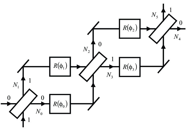
Figure 10: Diagram of a DLM network that simulates single-photon propagation through two chained Mach-Zehnder interferometers on an event-by-event basis.

The network shown in Fig.8 has two input channels (0 and 1) and two output channels (0 and 1). The network receives events at one of the two input channels. Each input event carries information in the form of a two-dimensional unit vector. Either input channel 0 receives $(y_{1,n+1},y_{2,n+1})$ or input channel 1 receives $(y_{3,n+1},y_{4,n+1})$. The input is fed into the device described in Section II.5. The purpose of this front-end DLM is to transform the information contained in two-dimensional input vectors (of which only one is present for any given input event), into a four-dimensional unit vector. The four-dimensional internal vector of this device is split into two groups of two-dimensional vectors $(\widetilde{x}_{1,n+1},\widetilde{x}_{4,n+1})$ and $(\widetilde{x}_{3,n+1},\widetilde{x}_{2,n+1})$ and each of these two-dimensional vectors is rotated by $45^{\circ}$. Put differently, the four-dimensional vector is rotated once in the (1,4)-plane about $45^{\circ}$ and once in the (3,2) plane about $45^{\circ}$. The order of the rotations is irrelevant. The resulting four-dimensional vector is then sent to the input of a second $K=4$ DLM. This back-end DLM sends $(x_{1,n+1},x_{2,n+1})/\sqrt{x_{1,n+1}^{2}+x_{2,n+1}^{2}}$ through output channel 0 if it used rule $j=1,2$ (see Eq. (17)) to update its internal state. Otherwise it sends $(x_{3,n+1},x_{4,n+1})/\sqrt{x_{3,n+1}^{2}+x_{4,n+1}^{2}}$ through output channel 1.

The operation of the network depicted in Fig.8 can be analyzed analytically if we disregard transient effects and assume that the information carried by events on channel 0 (1) is given by ${\bf y}_{n+1}={\bf y}=(y_{1},y_{2})$ (${\bf y}^{\prime}_{n+1}={\bf y}^{\prime}=(y_{3},y_{4})$). We denote by $p$ the number of events on input channel 0 divided by the total number of events. Then, the number of events on input channel 1 is given by $1-p$.

In the stationary regime, the internal state $(\widetilde{x}_{1,n+1},\widetilde{x}_{2,n+1},\widetilde{x}_{3,n+1},\widetilde{x}_{4,n+1})$ of the front-end DLM (see Fig.8) learns $(w_{1},w_{2},w_{3},w_{4})=(y_{1}\sqrt{p},y_{2}\sqrt{p},y_{3}\sqrt{1-p},y_{4}\sqrt{1-p})$. Carrying out the two plane rotations of $45^{\circ}$ we see that the back-end DLM receives as input the four-dimensional vector $(w_{1}-w_{4},w_{3}+w_{2},w_{3}-w_{2},w_{1}+w_{4})/\sqrt{2}$. In the stationary regime, the internal vector $(x_{1,n+1},x_{2,n+1},x_{3,n+1},x_{4,n+1})$ of the back-end DLM oscillates about $(w_{1}-w_{4},w_{3}+w_{2},w_{3}-w_{2},w_{1}+w_{4})/\sqrt{2}$. Therefore, in the stationary regime and for fixed two-dimensional vectors on input channels 0 and 1, the input-output relation of the BS network of Fig. 8 can be written as

$$\left(\begin{array}[]{c}w_{1}\\ w_{2}\\ w_{3}\\ w_{4}\end{array}\right)\overset{BS}{\longrightarrow}\frac{1}{\sqrt{2}}\left(\begin{array}[]{c}w_{1}-w_{4}\\ w_{3}+w_{2}\\ w_{3}-w_{2}\\ w_{1}+w_{4}\end{array}\right).$$ (42)

Using two complex numbers instead of four real numbers Eq. (42) can also be written as

$$\left(\begin{array}[]{c}w_{1}+iw_{2}\\ w_{3}+iw_{4}\end{array}\right)\overset{BS}{\longrightarrow}\frac{1}{\sqrt{2}}\left(\begin{array}[]{c}w_{1}-w_{4}+i(w_{3}+w_{2})\\ w_{3}-w_{2}+i(w_{1}+w_{4})\end{array}\right).$$ (47)

In quantum theory QuantumTheory the presence of photons in the input modes 0 or 1 is represented by the probability amplitudes ($a_{0},a_{1})$ BAYM74 ; GRAN86 ; RARI97 ; NIEL00 . According to quantum theory QuantumTheory , the probability amplitudes ($b_{0},b_{1})$ of the photons in the output modes 0 and 1 of a beam splitter are given by BAYM74 ; GRAN86 ; RARI97 ; NIEL00

$$\left(\begin{array}[]{c}b_{0}\\ b_{1}\end{array}\right)=\left(\begin{array}[]{c}a_{0}+ia_{1}\\ a_{1}+ia_{0}\end{array}\right)=\frac{1}{\sqrt{2}}\left(\begin{array}[]{cc}1&i\\ i&1\end{array}\right)\left(\begin{array}[]{c}a_{0}\\ a_{1}\end{array}\right).$$ (56)

Identifying $a_{0}$ with $w_{1}+iw_{2}=(y_{1}+iy_{2})p$ and $a_{1}$ with $w_{3}+iw_{4}=(y_{3}+iy_{4})(1-p)$ it is clear that by construction, the DLM network in Fig. 8 will allow us to simulate a beam splitter, not by calculating the amplitudes Eq. (56) but by a deterministic event-by-event simulation.

In Fig. 8 (right) we present results of discrete-event simulations using the DLM network depicted in Fig. 8 (left). Before the simulation starts, the internal vectors of the DLMs are given a random value (on the unit sphere). Each data point represents 10000 events. All these simulations were carried out with $\alpha=0.99$. For each set of 10000 events, a uniform random number in the range $[0,360]$ generates two angles $\psi_{0}$ and $\psi_{1}$. Input channel 0 receives $(y_{1,n+1},y_{2,n+1})=(\cos\psi_{0},\sin\psi_{0})$ with probability $p_{0}$. Input channel 1 receives $(y_{3,n+1},y_{4,n+1})=(\cos\psi_{1},\sin\psi_{1})$ with probability $p_{1}=1-p_{0}$. Random processes only enter in the procedure to generate the input data. The DLM network processes the events sequentially and deterministically. From Fig. 8 it is clear that the output of the deterministic DLM-based beam splitter reproduces the probability distributions as obtained from quantum theory QuantumTheory .

Figure 11: Absolute value of the difference between the normalized intensity $N_{4}/(N_{4}+N_{5})$ in output channel 0 of the event-based DLM simulation and the result of quantum theory QuantumTheory for the system of two chained Mach-Zehnder interferometers shown in Fig. 10 MZIdemo . Input channel 0 receives $(y_{1,n+1},y_{2,n+1})=(\cos\psi_{0},\sin\psi_{0})$ with probability $p_{0}$. Input channel 1 receives $(y_{3,n+1},y_{4,n+1})=(\cos\psi_{1},\sin\psi_{1})$ with probability $1-p_{0}$. For each event a uniform random number in the range $[0,360]$ determines $\psi_{0}$ or $\psi_{1}$. Each data point represents a simulation of 10000 events ($N_{0}+N_{1}=N_{2}+N_{3}=N_{4}+N_{5}=10000$). Top-left: Difference as a function of $p_{0}$; Top-right: Difference as a function of $\psi_{0}-\psi_{1}$; Bottom-left: Difference as a function of $\phi_{0}-\phi_{1}$; Bottom-right: Difference as a function of $\phi_{2}-\phi_{3}$.

Figure 12: Same as Fig. 11 except that $\alpha=0.9999$ (instead of $\alpha=0.99$) and that the 1000000 events (instead of 10000) per data point were processed by the DLM network depicted in Fig. 10.

IV.3 Mach-Zehnder interferometer

In quantum physics QuantumTheory , single-photon experiments with one beam splitter provide direct evidence for the particle-like behavior of photons GRAN86 ; HOME97 . The wave mechanical character appears when one performs single-particle interference experiments. In this subsection we construct a DLM network that displays the same interference patterns as those observed in single-photon Mach-Zehnder interferometer experiments GRAN86 .

The schematic layout of the DLM network is shown in Fig. 9. Not surprisingly, it is exactly the same as that of a real Mach-Zehnder interferometer. The BS network described in the previous subsection is used for the beam splitters. The phase shift is taken care of by a passive device that performs a plane rotation. Clearly there is a one-to-one mapping from each relevant component in the interferometer to a processing unit in the DLM network. Recall that the processing units in the DLM network only communicate with each other through the message (photon) that propagates through the network.

According to quantum theory QuantumTheory , the probability amplitudes ($b_{0},b_{1})$ of the photons in the output modes 0 ($N_{2}$) and 1 ($N_{3}$) of the Mach-Zehnder interferometer are given by BAYM74 ; GRAN86 ; RARI97 ; NIEL00

$$\left(\begin{array}[]{c}b_{0}\\ b_{1}\end{array}\right)=\frac{1}{2}\left(\begin{array}[]{cc}1&i\\ i&1\end{array}\right)\left(\begin{array}[]{cc}e^{i\phi_{0}}&0\\ 0&e^{i\phi_{1}}\end{array}\right)\left(\begin{array}[]{cc}1&i\\ i&1\end{array}\right)\left(\begin{array}[]{c}a_{0}\\ a_{1}\end{array}\right).$$ (67)

Note that in a quantum mechanical setting it is impossible to simultaneously measure ($N_{0}/(N_{0}+N_{1})$, $N_{1}/(N_{0}+N_{1})$) and ($N_{2}/(N_{0}+N_{1})$, $N_{3}/(N_{0}+N_{1})$): Photon detectors operate by absorbing photons. However, in our deterministic, event-based simulation there is no such problem.

In Fig. 9 we present a small selection of simulation results for the Mach-Zehnder interferometer built from DLMs. We assume that input channel 0 receives $(y_{1,n+1},y_{2,n+1})=(\cos\psi_{0},\sin\psi_{0})$ with probability one and that input channel 1 receives no events. This corresponds to $(a_{0},a_{1})=(\cos\psi_{0}+i\sin\psi_{0},0)$. We use uniform random numbers to determine $\psi_{0}$. In all these simulations $\alpha=0.99$. The data points are the simulation results for the normalized intensity $N_{i}/(N_{0}+N_{1})$ for i=0,2,3 as a function of $\phi=\phi_{0}-\phi_{1}$. Lines represent the corresponding results of quantum theory QuantumTheory . From Fig. 9 it is clear that quantum theory provides an excellent description of the deterministic, event-based processing by the DLM network.

The examples presented in Fig. 9 do not rule out that there may be settings for the angles $\psi_{0}$, $\phi_{0}$ and $\phi_{1}$ for which quantum theory fails to give a good description of the behavior of the DLM network. However extensive series of simulations show that this is not the case. Instead of presenting the results of these simulations we will demonstrate that quantum theory QuantumTheory also describes the stationary-state input-output behavior of more extended DLM networks.

As an example we consider the DLM network depicted in Fig. 10. Obviously this network maps exactly onto two chained Mach-Zehnder interferometers MZIdemo . Now there are seven parameters $p_{0}$, $\psi_{0}$, $\psi_{1}$, $\phi_{0}$, $\phi_{1}$, $\phi_{2}$, and $\phi_{3}$ that may be varied, so simply plotting selected cases is not the proper procedure to establish that quantum theory describes the stationary-state behavior of the DLM network. Therefore we adopt the following strategy. For each set of 10000 events, we use seven random numbers to fix the parameters $p_{0}$, $\psi_{0}$, $\psi_{1}$, $\phi_{0}$, $\phi_{1}$, $\phi_{2}$, and $\phi_{3}$. Then we collect the data for these 10000 events and compare the intensity in output channel 0 ($N_{4}$) and 1 ($N_{5}$) with the corresponding results of quantum theory QuantumTheory . The latter is given by

$$\left(\begin{array}[]{c}b_{0}\\ b_{1}\end{array}\right)=\frac{1}{2\sqrt{2}}\left(\begin{array}[]{cc}1&i\\ i&1\end{array}\right)\left(\begin{array}[]{cc}e^{i\phi_{2}}&0\\ 0&e^{i\phi_{3}}\end{array}\right)\left(\begin{array}[]{cc}1&i\\ i&1\end{array}\right)\left(\begin{array}[]{cc}e^{i\phi_{0}}&0\\ 0&e^{i\phi_{1}}\end{array}\right)\left(\begin{array}[]{cc}1&i\\ i&1\end{array}\right)\left(\begin{array}[]{c}a_{0}\\ a_{1}\end{array}\right).$$ (82)

For each choice of $\{p_{0},\psi_{0},\psi_{1},\phi_{0},\phi_{1},\phi_{2},\phi_{3}\}$ we compute the differences $||b_{0}|^{2}-N_{4}/(N_{4}+N_{5})|$ and $||b_{1}|^{2}-N_{5}/(N_{4}+N_{5})|$. $N_{4}$ ($N_{5}$) is the number of events in the output channel 0 (1) of the third beam splitter. $N_{0}+N_{1}=N_{2}+N_{3}=N_{4}+N_{5}$ is the total number of events (10000 in this case). In Fig. 11 we show $||b_{0}|^{2}-N_{4}/(N_{4}+N_{5})|$ as a function of $p_{0}$, $\psi_{0}-\psi_{1}$, $\phi_{0}-\phi_{1}$, and $\phi_{2}-\phi_{3}$. In all these simulations $\alpha=0.99$. Once again it is clear that quantum theory QuantumTheory provides a very good description of a DLM-based simulation of two chained Mach-Zehnder interferometers.

IV.4 Technical note

All simulations that we presented in this section have been performed for $\alpha=0.99$. From the description of the learning process it is clear that $\alpha$ controls the rate of learning or, equivalently, the rate at which learned information can be forgotten. Furthermore it is evident that the difference between a constant input to a DLM and the learned value of its internal variable cannot be smaller than $1-\alpha$. In other words, $\alpha$ also limits the precision with which the internal variable can represent a sequence of constant input values. On the other hand, the number of events has to balance the rate at which the DLM can forget a learned input value. The smaller $1-\alpha$ is, the larger the number of events has to be for the DLM to adapt to changes in the input data.

We use the last example of Section IV.3 to illustrate the effect of changing $\alpha$ and the total number of events $N$. In Fig. 12 we show the results of repeating the procedure used to obtain the data shown in Fig. 11 but instead of $\alpha=0.99$ and $N=10000$ events per data point, we used $\alpha=0.9999$ and $N=1000000$ event per data point. As expected, the difference between the simulation data and the results of quantum theory decreases if $1-\alpha$ decreases and $N$ increases accordingly. Comparing Fig. 11 with Fig. 12 it is clear that the decrease of this difference is roughly proportional to the inverse of the square root of the number of events. Note that each data point in Fig. 11 is generated without the use of random processes.

Figure 13: Simulation results for a Mach-Zehnder interferometer built from SLMs instead of DLMs. Each beam splitter sends messages over its output channels 0 and 1 in a random manner. The simulation procedure and annotations are exactly the same as in Fig. 9.

V Stochastic learning machines

In the stationary regime, the sequence of messages that a DLM (network) generates is strictly deterministic. For some applications, e.g. for quantum physics QuantumTheory , it may be desirable to randomize these sequences. A marginal modification turns a DLM into a stochastic learning machine (SLM). Here the term stochastic does not refer to the learning process but to the method that is used to select the output channel that will carry the outgoing message.

In the stationary regime the components of the internal vector represent the probability amplitudes. Comparing the (sums of) squares of these amplitudes with a uniform random number $0<r<1$ gives the probability for sending the message over the corresponding output channel. For instance, in the case of the beam splitter BS (see Fig. 8) we replace the back-end DLM by a SLM. This SLM will send a message over output channel 0 if $x^{2}_{1,n+1}+x^{2}_{2,n+1}\leq r$. Otherwise it will activate output channel 1. Although the learning process of this modified BS network is still deterministic, in the stationary regime the output messages are randomly distributed over the two output channels. Of course, the distribution of output messages is the same as that of the original DLM-network.

Replacing DLMs by SLMs in a DLM-network changes the order in which messages are being processes by the network but leaves the content of the messages intact. Therefore, in the stationary regime, the distribution of messages over the outputs of the SLM-network is essentially the same as that of the original DLM network.

As an illustration of the use of SLMs, we replace the two back-end DLMs in the Mach-Zehnder interferometer network (see Fig. 9 (left)) by their “randomized” version and repeat the procedure that generates the data of Fig. 9 (right). The results of these simulations are shown in Fig. 13. Not unexpectedly, the randomness in the output channel selection is reflected by a (small) increase of the scatter on the data points. In this simulation, the output channels 0 and 1 of each beam splitter are activated in a random manner and the functional dependence of $N_{0}/(N_{0}+N_{1})$, $N_{1}/(N_{0}+N_{1})$, $N_{2}/(N_{2}+N_{3})=N_{2}/(N_{0}+N_{1})$ and $N_{3}/(N_{2}+N_{3})$ on $\phi$ is still in full agreement with quantum theory QuantumTheory . In other words, this SLM-network performs a genuine, event-by-event simulation of the ideal (perfect detectors, etc.) version of both the single-photon beam splitter and Mach-Zehnder interferometer experiments by Grangier et al GRAN86 .

VI Discussion

We have proposed a new procedure to construct deterministic algorithms that have primitive learning capabilities. We have used these algorithms to build deterministic learning machines (DLMs). A DLM learns by processing event after event but does not store the data contained in an individual event. Connecting the input of a DLM to the output of another DLM yields a locally connected network of DLMs. A DLM within the network locally processes the information contained in an event and responds by sending a message that may be used as input for another DLM. A distinct feature of a DLM network is that at any given time, only one event (message) is propagating through the network. The DLMs process messages in a sequential manner and only communicate with each other by message passing.

We have demonstrated that DLM networks can discover relationships between successive events (see Section III) and that certain classes of DLM networks exhibit behavior that is usually only attributed to quantum systems. In Sections IV and V we have presented DLM networks that simulate quantum interference on an event-by-event basis. More specifically, we map each physical part of the real Mach-Zehnder interferometer onto a DLM and the messages (phase shifts in this case) are carried by photons. No ingredient other than simple geometry is used to specify the update rules of the DLMs.

As the network processes event after event, the network generates output events that build an interference pattern that is described by the quantum theory QuantumTheory of the single-photon beam splitter and Mach-Zehnder interferometer. To illustrate that DLM networks are indeed capable of simulating quantum interference on an event-by-event basis we also simulate an experiment involving three beam splitters (i.e. two chained Mach-Zehnder interferometers) and demonstrate that quantum theory QuantumTheory also describes the behavior of this network.

The results presented in Sections IV and V suggest that we may have discovered a systematic procedure to construct algorithms that simulate quantum phenomena using deterministic, local, and event-by-event-based processes. We emphasize that our approach is not a proposal for another interpretation of quantum mechanics. Our approach is not an extension of quantum theory in any sense: The probability distributions of quantum theory appear as the result of a deterministic, causal learning process, and not vice versa (see Section IV) PENR90 . Our results suggest that quantum mechanical behavior may originate from an underlying deterministic process tHOO01 ; tHOO02 . Indeed, it is somewhat ironic that in order to mimic the apparent randomness with which events are observed in experiments, we have to explicitly randomize the output of the DLMs to mask the underlying deterministic processes (see Section V). To the best of our knowledge, this paper contains the first demonstration that quantum interference can be simulated on an event-by-event basis using local, causal, and deterministic processes, and without using concepts such as wave fields or particle-wave duality.

At this point it may be worthwhile to recall what a DLM actually does. In a simple physical picture, a DLM is a device (e.g. beam splitter, polarizer) that exchanges information with the particles that pass through it. The DLM tries to do this in an effective manner. It learns by comparing the message carried by an event with predictions based on the knowledge acquired by the DLM during the processing of previous events. Effectively this comparison amounts to a minimization of the squared error (see Section II). Schrödinger used exactly the same principle to derive his famous equation SCHR26a but called this approach “unverständlich” in a subsequent publication SCHR26b .

In a future publication we will show that the approach introduced in this paper can be employed to perform event-based simulations of a universal quantum computer KRIS04 . It has been shown that the time evolution of the wave function of a quantum system can be simulated on a quantum computer ZALK98 ; NIEL00 . Therefore it should be possible to compute the real-time dynamics of these systems (including the double-slit experiment mentioned in the introduction) through discrete-event simulation by constructing appropriate DLM networks.

References

- (1) D.P. Landau and K. Binder, A Guide to Monte Carlo Simulation in Statistical Physics, Cambridge University Press, Cambridge, (2000)
- (2) A. Tonomura, The Quantum World Unveiled by Electron Waves, World Scientific, Singapore (1998)
- (3) In this paper we disregard limitations of real experiments such as detector efficiency, imperfection of the source, biprism etc.
- (4) D. Home, Conceptual Foundations of Quantum Physics, Plenum Press, New York (1997)
- (5) N.G. Van Kampen, Physica A 153, 97 (1988)
- (6) We make a distinction between quantum theory and quantum physics. We use the term quantum theory when we refer to the mathematical formalism, i.e., the postulates of quantum mechanics (with or without the wave function collapse postulate) BALL03 and the rules (algorithms) to compute the wave function. The term quantum physics is used for microscopic, experimentally observable phenomena that do not find an explanation within the mathematical framework of classical mechanics.
- (7) R.P. Feynman, R.B. Leighton, M. Sands, The Feynman lectures on Physics, Vol. 3, Addison-Wesley, Reading MA, (1996)
- (8) L.E. Ballentine, Quantum Mechanics: A Modern Development, World Scientific, Singapore (2003)
- (9) H. De Raedt, Computer Simulation of Quantum Phenomena in Nano-Scale Devices, Annual Reviews of Computational Physics IV, ed. D. Stauffer, World Scientific, 107 (1996)
- (10) A large collection of video’s of such simulations can be found at http://www.compphys.org/quantummechanics
- (11) R. Penrose, The Emperor’s New Mind, Oxford University Press, Oxford (1990)
- (12) P. Grangier, R. Roger, and A. Aspect, Europhys. Lett. 1, 173 (1986)
- (13) S. Haykin, Neural Networks, Prentice Hall, New Jersey (1999)
- (14) S. Haykin, Adaptive Filter Theory, Prentice Hall, New Jersey (1986)
- (15) K.V. Mardia, J.T. Kent, and J.M. Bibby, Multivariate Analysis, Academic Press, London (1982)
- (16) G.H. Golub and C.F. Van Loan, Matrix Computations, John Hopkins University Press, Baltimore (1996)
- (17) R.P. Feynman, Int. J. Theor. Phys. 21, 467 (1982)
- (18) G. Baym, Lectures on Quantum Mechanics, W.A. Benjamin, Reading MA (1974)
- (19) M. Born and E. Wolf, Principles of Optics, Pergamon, Oxford (1964)
- (20) An interactive program that performs the event-based simulations of a beam splitter, one Mach-Zehnder interferometer, and two chained Mach-Zehnder interferometers can be found at http://www.compphys.net/dlm
- (21) J.G. Rarity and P.R. Tapster, Phil. Trans. R. Soc. Lond. A 355, 2267 (1997)
- (22) M. Nielsen and I. Chuang, Quantum Computation and Quantum Information, Cambridge University Press, Cambridge (2000)
- (23) G. ’t Hooft, “Determinism beneath Quantum Mechanics”, quant-ph/0105105
- (24) G. ’t Hooft, “Quantum Mechanics and Determinism”, quant-ph/0212095
- (25) E. Schrödinger, Ann. Phys. 79, 361 (1926)
- (26) E. Schrödinger, Ann. Phys. 79, 491 (1926)
- (27) K. Michielsen, K. De Raedt, and H. De Raedt, in preparation.
- (28) C. Zalka, Proc. R. Soc. Lond. A454, 313 (1998)