Quantum mechanical description of Stern-Gerlach experiments

Abstract

The motion of neutral particles with magnetic moments in an inhomogeneous magnetic field is described in a quantum mechanical framework. The validity of the semi-classical approximations which are generally used to describe these phenomena is discussed. Approximate expressions for the evolution operator are derived and compared to the exact calculations. Focusing and spin-flip phenomena are predicted. The reliability of Stern-Gerlach experiments to measure spin projections is assessed in this framework.

I Introduction

The Stern-Gerlach experiment consists in taking a beam of particles that have a neutral electric charge, but a finite magnetic moment, and passing them through an inhomogeneous magnetic field. The observed result is that the particles deflect differently depending on the spin projection along the magnetic field. So, by measuring the deflection, one can infer the value of the spin projection of the particles along the direction of the magnetic field. The description of this phenomenon is done with the following assumptions:

i) The spin projection along the z-axis, taken along the magnetic field at the centre of the beam, is conserved.

ii) Particles with different spin projections along the z-axis, as they go through the inhomogeneous magnetic field, suffer a force in the z-direction that is given by the product of the magnetic moment times the gradient of the field times the spin projection.

This is what we will call the text-book description of the Stern-Gerlach experiment eis ; lev ; mer ; mes . Thus, considering the particle position as a pointer, and the spin projection as the quantum property to be measured, the Stern-Gerlach setup is associated to a measurement operator on the spin state which has as eigenvalues the spin projections along the z-axis. Under the text-book description, the Stern Gerlach experiment corresponds to an “ideal” measurement, in the sense of von Neumann neumann , because the quantum state is not modified by the measurement process when it is an eigenstate of the measuring apparatus. Besides, it is “completely reliable”, in the sense discussed in bassi , because the the position is completely correlated with the spin projection.

However, when the experiment is investigated in more detail, the situation becomes more complicated. As the magnetic field has zero divergence, then it is not possible to have a gradient of the field only in one direction. This produces terms in the Hamiltonian that can change the spin of the incident particle. A detailed investigation of these effects was made in a recent publication prasara , making use of the concept of coherent internal states sara in a semi-classical approach. The main results of that paper was that, indeed, when a beam of particles goes through a Stern-Gerlach magnet, the different spin projections deviate depending on the spin projection. However, when the size of the beam is not very small compared to the range of inhomogeneity of the magnetic field, additional effects occur.

i) There is a focusing effect, so that the particles deviating in the direction in which the field decreases tend to focus, while those going in the direction of increasing field tend to de-focus.

ii) There are some particles with a given spin projection which deviate as those with a different spin projection. So, the Stern-Gerlach setup is not, even in theory, a “completely reliable” measuring apparatus.

iii) There are some particles, with a definite spin projection along the quantisation axis, which change the spin projection as they go through the magnet. So, the Stern-Gerlach setup is not an “ideal” measurement apparatus, as successive measurements will not give exactly the same results.

This is what we will call the semi-classical description of the Stern-Gerlach experiment. Note that if we associate the particle position after the magnet as a “pointer”, which gives the result of the measurement of the spin projection along the z-axis, then we conclude, that, in the semi-classical description, the Stern-Gerlach experiment is not an ideal measurement, because it can alter the spin projection, nor a completely reliable one, because the position is not always correlated with the spin projection.

These conclusions were obtained in a semi-classical framework, in which the motion of the particles was described by classical trajectories which depended in the spin projection along the magnetic field that they encountered. Our motivation here is to see whether the same conclusions hold when the full quantum mechanical problem is considered. In section 2 we formulate the time dependent quantum mechanical problem of a wave packet going through a Stern-Gerlach magnet, and discuss the validity of the text-book and semi-classical approaches. In section 3 and present the numerical solution of the quantum-mechanical problem. In section 4 we investigate several analytic approximations to the problem, considering the validity of the concept of coherent internal states. In section 5 we discuss the interpretation of Stern-Gerlach experiments as measurements devices. Section 6 is for summary and conclusions.

II Quantum mechanical formulation

We want to investigate the effect of an inhomogeneous magnetic field on the evolution of a quantum wave-packet. The situation that we will consider is a magnetic field that has components in the $X$ and $Z$ directions, but not in the $Y$ direction. This magnetic field has a length $L$, and it can be written as

$$\vec{B}=(B_{0}+B_{1}Z)\vec{u}_{z}-B_{1}X\vec{u}_{x}\quad,\quad 0\leq Y\leq L\quad.$$ (1)

We use the capital letters $X,Y,Z,T$ to represent magnitudes with dimensions. Low case $x,y,z,t$ correspond to dimensionless quantities. We neglect border effects around $Y=0$ or $Y=L$. Note that this field fulfils $\nabla\vec{B}=0$, and also $\nabla\times\vec{B}=0$, as it should be expected for a magnetic field in the region where there are no currents. These conditions were not fulfilled in the case discussed in textbooks such as eis ; lev ; mer .

The Hamiltonian which describes a non-relativistic neutral particle which enters in this field is given by

$${\cal H}={P_{X}^{2}+P_{Y}^{2}+P_{Z}^{2}\over 2M}-\mu\vec{B}\cdot\vec{I}\quad,$$ (2)

where $\mu$ is the magnetic moment and $\vec{I}$ is the spin operator.

We consider now a wave packet $|\Psi(T);m_{0}\rangle$ which enters into this field. Initially, the wave packet can be characterised in coordinate space as a Gaussian which is moving in the y-direction, while the initial spin projection along the $Z$-axis is $m_{0}$.

$$\langle XYZ,m|\Psi(T=0);m_{0}\rangle=N\exp(-{X^{2}+Y^{2}+Z^{2}\over 2\sigma^{2}})\exp(ik_{y}Y)\delta(m,m_{0})\quad.$$ (3)

Note that, neglecting the effects of the border, the $Y$-component of the wave-function is not affected by the interaction. On the other hand, the wave-function can be factorized into a $Y$-component and an $(X,Z)$-component. The former component will evolve freely inside the magnet. Note that the wave-packet will stay within the magnetic field during a time $\tau=L/v_{y}$, where $v_{y}=\hbar k_{y}/M$. Assuming that the size of the wave-packet $\sigma$ is very small compared to $L$, we can consider that the magnetic field starts at $T=0$, and finishes at $T=\tau$. So, we focus on solving the two-dimensional time dependent problem, which corresponds to calculate the time evolution between the time $T=0$ and $T=\tau$ in a Hamiltonian

$${H}={P_{X}^{2}+P_{Z}^{2}\over 2M}-\mu\vec{B}\cdot\vec{I},$$ (4)

considering that the initial wave-function is

$$\langle XZ;m|\Phi(T=0);m_{0}\rangle=N\exp(-{X^{2}+Z^{2}\over 2\sigma^{2}})\delta(m,m_{0})\quad.$$ (5)

It is convenient to make use of dimensionless variables. So, we define $x=X/\sigma$, $z=Z/\sigma$, $t=T/\tau$, $h=H\tau/\hbar$. Then, the equation of motion becomes

$$h|\Phi(t);m_{0}\rangle=i{d\over dt}|\Phi(t);m_{0}\rangle.$$ (6)

The dimensionless Hamiltonian can be written as $h=h_{0}+v$, with

$$h_{0}={A\over 2}\left(p_{x}^{2}+p_{z}^{2}\right)\quad;\quad v=-S\left(I_{z}(z+z_{0})-I_{x}x\right)\quad.$$ (7)

where $p_{x}=-id/dx$, $p_{z}=-id/dz$, and the dimensionless parameters $A,S,z_{0}$ are

$$A={\hbar\tau\over M\sigma^{2}}\quad;\quad S={\mu B_{1}\tau\sigma\over\hbar}\quad;\quad z_{0}={B_{0}\over\sigma B_{1}}\quad.$$ (8)

The adiabaticity parameter $A$ is the ratio of the interaction time $\tau$ to the natural time of expansion of the Gaussian packet. The separation parameter $S$ is the ratio of the momentum change induced by the magnetic field gradient divided by the momentum width of the Gaussian packet. The inhomogeneity parameter $z_{0}$ determines the relative change of the magnetic field in the range of the Gaussian. Note that in the position $(x=0,z=-z_{0})$, the magnetic field vanishes. Note that the product $AS=\mu B_{1}\tau^{2}/M\sigma$ is independent of $\hbar$. This magnitude is related to the deviation of the beam in the magnet. For a given trajectory, which is determined by a fixed value of the product $AS$, the classical limit is reached as $S\to\infty$ and $A\to 0$. Note that this corresponds to making $\hbar\to 0$ in eqs. 8.

II.1 Validity of the semi-classical descriptions

We will discuss the validity of the semi-classical and text-book descriptions of the Stern-Gerlach experiment. It should be noticed that, in general, a beam of particles is not given by a pure quantum mechanical state, but rather by a mixture of small quantum wave packets. For definiteness, we consider that initially one has a distribution of particles described as a Gaussian mixture, of range $\sigma_{m}$, of small Gaussian wave packets of range $\sigma$. The beam profile will then be characterised by a Gaussian of range $\sigma_{t}=\sqrt{\sigma_{m}^{2}+\sigma^{2}}$. The conditions required, in order to justify the semi-classical description done in prasara are the following:

a) The inhomogeneity of the magnetic field over the quantum size of the wave packet should be small: $\sigma B_{1}\ll B_{0}$. This implies that $z_{0}\gg 1$.

b) The momentum change should be large compared to the quantum spread of the beam momentum: $\mu B_{1}\tau\gg{\hbar/\sigma}$. This implies that $S\gg 1$.

Note that these conditions are very well satisfied in realistic situations for Stern-Gerlach experiments. However, the validity of the text-book description requires also the far more stringent condition $\sigma_{t}B_{1}\ll B_{0}$, which require very strong field $B_{0}$, or, alternatively, a very thin beam.

The purpose of this work is to investigate the full quantum solution of this problem for values of the parameters $z_{0},S$ which are not necessarily very large, so that the semi-classical and text-book description become dubious. Nevertheless, in order to have a reference to compare the quantum calculation, we remind the expected results in the text-book description. The trajectory of the centre of the wave packet inside the magnet, is given by the expression

$$z_{m}(t)=1/2(SA)mt^{2}\quad.$$ (9)

which depends on the spin projection $m$. Note that, after the interaction ($t=1$), the positions of the centre of the wave packets for each spin projection are given by $z_{m}(1)=SAm/2$, and their velocities are $\dot{z}_{m}(1)=SAm/2$. If, after the interaction, the beam evolves freely during a time $t_{d}$, then the positions of the centre of the wave packets are expected to be given by

$$z_{m}(t_{d})=(1/2+t_{d})(SA)m\quad.$$ (10)

As a typical value of the drift time $t_{d}$ we will consider the time necessary to reach the position $z_{m}=-z_{0}$, for the spin projection $m=-1/2$. Thus,

$$t_{d}=2z_{0}/(SA)-1/2\quad.$$ (11)

Thus, we would expect that, after a drift time $t_{d}$, particles with spin projection $m=1/2$ should appear around $z=z_{0},x=0$, and particles with spin projection $m=-1/2$ should appear around $z=-z_{0},x=0$.

III Numerical calculations

We consider the scattering of a spin $1/2$ particle. We expand the wave-function into two components, which have definite spin projections along the z-axis.

$$\langle xz;m=1/2|\Phi(t);m_{0}\rangle = \alpha(x,z,t)e^{itSz_{0}/2}$$

$$\langle xz;m=-1/2|\Phi(t);m_{0}\rangle = \beta(x,z,t)e^{-itSz_{0}/2}$$ (12)

and the Schrödinger equation for the (x,z) plane can be written as

$$\left[\begin{array}[]{cc}{A\over 2}\left(p_{x}^{2}+p_{z}^{2}\right)-{S\over 2}z&{S\over 2}x\\ {S\over 2}x&{A\over 2}\left(p_{x}^{2}+p_{z}^{2}\right)+{S\over 2}z\\ \end{array}\right]\left[\begin{array}[]{c}\alpha(x,z,t)\\ \beta(x,z,t)\\ \end{array}\right]=i{d\over dt}\left[\begin{array}[]{c}{\alpha}(x,z,t)\\ {\beta}(x,z,t)\\ \end{array}\right]$$ (13)

where $\alpha(x,z,t)$ and $\beta(x,z,t)$ are the components of the spinor in the basis of the eigenstates of $I_{z}$. The numerical solution of this equation has already been performed by Garraway and Stenholm garraway . However, they considered the case in which $z_{0}$ was large, so their numerical result corresponded to the text-book interpretation. A similar problem has been addressed by Franca et al franca , but they made use of the adiabatic approximation, neglecting the kinetic energy during the interaction time.

To follow our approach we must first write both components of the spinor as linear combinations of harmonic oscillator functions, so that

$$\alpha(x,z,t) = \sum_{nm}a_{nm}(t)\phi_{n}(x)\phi_{m}(z)\rangle$$

$$\beta(x,z,t) = \sum_{nm}b_{nm}(t)\phi_{n}(x)\phi_{m}(z),$$ (14)

where $\phi_{n}(x)$ and $\phi_{m}(z)$ are the harmonic oscillator eigenstates of order $n,m$ in the $x$ and in the $z$ direction respectively. To calculate the time-dependent coefficients $a_{nm}(t)$ and $b_{nm}(t)$ of the expansion, it is natural to rewrite the equation 13 in terms of the well known creation and destruction operators:

$$a_{x}=\frac{1}{\sqrt{2}}(x+ip_{x})\quad \quad a^{\dagger}_{x}=\frac{1}{\sqrt{2}}(x-ip_{x})$$

$$a_{z}=\frac{1}{\sqrt{2}}(z+ip_{z})\quad \quad a^{\dagger}_{z}=\frac{1}{\sqrt{2}}(z-ip_{z})$$ (15)

Thus, substituting the operators III in eq. 13, we obtain the desired system of ordinary coupled differential equations for the coefficients of the expansion of $\alpha(x,z,t)$ and $\beta(x,z,t)$:

$$\dot{a}_{nm}=i\frac{A}{4}\left(a_{n+2,m}\sqrt{(n+1)(n+2)}+a_{n-2,m}\sqrt{n(n-1)}+\right.$$

$$\left.a_{n,m+2}\sqrt{(m+1)(m+2)}+a_{n,m-2}\sqrt{m(m-1)}-2a_{nm}(n+m+1)\right)+$$

$$i\frac{S}{2\sqrt{2}}\left(a_{n,m+1}\sqrt{m+1}+a_{n,m-1}\sqrt{m}-\left(b_{n+1,m}\sqrt{n+1}+b_{n-1,m}\sqrt{n}\right)e^{-iSz_{0}t}\right)$$

$$\dot{b}_{nm}=i\frac{A}{4}\left(b_{n+2,m}\sqrt{(n+1)(n+2)}+b_{n-2,m}\sqrt{n(n-1)}+\right.$$

$$\left.b_{n,m+2}\sqrt{(m+1)(m+2)}+b_{n,m-2}\sqrt{m(m-1)}-2b_{nm}(n+m+1)\right)+$$

$$i\frac{S}{2\sqrt{2}}\left(-b_{n,m+1}\sqrt{m+1}-b_{n,m-1}\sqrt{m}-\left(a_{n+1,m}\sqrt{n+1}+a_{n-1,m}\sqrt{n}\right)e^{iSz_{0}t}\right),$$

where the dot stands for differentiation with respect to the dimensionless parameter $t$. This system is solved using a fourth order Runge-Kutta method. The number of harmonic oscillator basis functions needed in the calculation was typically of the order of 40 in each coordinate.

We have performed calculations using typical values of $A=0.5$, $S=4$, $z_{0}=4$. This corresponds to a case in which the magnetic field vanishes at a distance of $4\sigma$ . The time of the interaction is such that the width of the beam would increase by a factor $\sqrt{1+A^{2}}$. The magnetic field gradient is such that each component of the magnetic field will acquire a momentum of $S\hbar/2\sigma$, in opposite directions. As a comparison, we have also considered calculations with $A=0.1$, $S=20$, $z_{0}=4$, that produce the same deviation of the beam, but are closer to the classical limit.

After the interaction, we consider a drift time $t_{d}$, given by eq. (11), during which the system evolves in the free Hamiltonian, so that the centre of the $m=\pm 1/2$ wave-packet would reach the point $z=\pm z_{0}$, according to the text-book description.

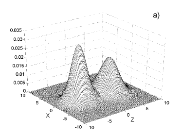
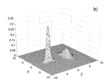
Figure 1: Probability distribution for an unpolarised wave packet after going through an inhomogeneous a magnetic field. Note the focusing effect of the lower component, which corresponds predominantly to $m=-1/2$. The upper figure correspond to A=0.5, S=4. The lower figure is for A=0.1, S=20, which is closer to the classical limit

In figure 1 we represent the probability distribution of a wave packet, corresponding initially to an unpolarised beam. This is given by

$$P_{0}(x,z)={1\over 2}\sum_{mm_{0}}|\langle x,z;m|\Phi(t);m_{0}\rangle|^{2}$$ (17)

The focusing effect can be clearly seen, by comparing the shape of the distributions for the upper and lower components, which correspond predominantly to $m=1/2$ and $m=-1/2$ respectively. The effect of the focusing is increased as $A$ decreases and $S$ increases. So, we have confirmed that the focusing effect that was predicted in the semi-classical calculation in sara is a genuine result, that appears in the quantum mechanical calculation, although it is diffused if the adiabaticity parameter $A$ has a sizeable value. It should be noticed that this focusing effect was also found in the calculations presented in garraway .

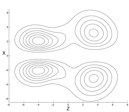
Figure 2: Contour plot of the probability distribution of the spin flip component (spin up to spin down) of the wave-function. The maximum is $3.3\cdot 10^{-4}$

In contrast to the text book description, even if the initial beam has a definite spin projection along the z-axis, after the scattering process this spin projection can change. We have evaluated the probability that the particles change their spin projection along the z-axis. It should be noticed that the probability of going from spin up to spin down is not exactly the same of that of going from spin down to spin up. For the reference case ($A=0.5,S=4,z_{0}=4$), we obtain that $p(1/2,-1/2)=0.0166$, $p(-1/2,1/2)=0.0198$.

The spin-flip phenomenon also appears in the semi-classical description, because not all the particles that compose the beam see the magnetic field along the z-axis. The semi-classical spin-flip probability is $p(1/2,-1/2)=p(-1/2,1/2)=0.0156$, which depends only on the value of $z_{0}$. This is in good qualitative agreement with the quantum calculations. In Fig 2 we represent the spatial distribution of the spin flip probability. Note that the spin flip probability vanishes for particles coming out along the z-axis. The spatial distribution of the spin-flip probability is in qualitative agreement with the semi-classical calculation, which becomes more accurate as one makes the limit $A\to 0$, $S\to\infty$, with $AS$ constant.

The results of our calculations can be summarised as follows: When a beam of particles, described by a Gaussian wave-function, and with a given spin projection along the z-axis goes through an inhomogeneous magnetic field, most of the particles scatter as expected in the text-book description. However, a sizeable fraction of them, which depends on $z_{0}$ (about 2% for $z_{0}=4$), suffer a change of the spin projection (spin flip). From these particles that suffer spin flip, about half scatter in the same direction as the majority of the particles, and the other half scatter in the opposite direction. We can conclude that the spin flip effect described in the semi-classical description, which was not present in the text book description of Stern-Gerlach experiments, is supported by the full quantum mechanical calculations. Also, we confirm that the Stern-Gerlach experiment, when considered as a measurement apparatus of the spin projection, is not an ideal measurement (because there is spin-flip) and it is not fully reliable (because there is not an exact correlation between the initial spin projection and the final position of the particle).

However, there are qualitative features of the full quantum mechanical result, such as the difference between up-down and down-up spin flip probabilities, that are not present in the semi-classical description and require further investigation.

IV Approximate treatments

Having solved numerically the problem, we will consider several approximate treatments to improve our understanding of the phenomena under consideration. The starting point is the exact evolution operator and the free evolution operator:

$$U(t)=\exp(-i(h_{0}+v)t)\quad;\quad U_{0}(t)=\exp(-ih_{0}t)\quad.$$ (18)

It should be noticed that $h_{0}$ and $v$ do not commute. We can use the following coordinates

$$\rho=\sqrt{(z+z_{0})^{2}+x^{2}}\quad,\quad\beta=\arctan{x\over(z+z_{0})}\quad,$$ (19)

and refer the spin components to the direction of the magnetic field at each position

$$I_{B}=I_{z}\cos(\beta)-I_{x}\sin(\beta)\quad;\quad I_{T}=I_{z}\sin(\beta)+I_{x}\cos(\beta)\quad.$$ (20)

In terms of these variables, the initial state can be expressed as

$$\langle\rho\beta;m|\Phi(t=0);m_{0}\rangle=N\exp(-{\rho^{2}-2\rho z_{0}\cos{\beta}+z_{0}^{2}\over 2})\delta(m,m_{0})$$ (21)

and $h_{0}$ and $v$ take the expressions

$$h_{0}={A\over 2}(p_{\rho}^{2}+\rho^{-2}p_{\beta}^{2}),\quad v=-S\rho I_{B}$$ (22)

where $p_{\rho}$ and $p_{\beta}$ are the momenta associated to $\rho$ and $\beta$. The relevant commutators are the following:

$$\quad[h_{0},v] = iAS(p_{\rho}I_{B}-\{p_{\beta},I_{T}\}/2\rho)$$

$$\quad[[h_{0},v],v] = -AS^{2}(I_{B}^{2}+I_{T}^{2}-\{p_{\beta},I_{y}\}/2$$ (23)

Note that $[[h_{0},v],h_{0}]=0$ and $[[[h_{0},v],v],h_{0}]=0$. For spin-1/2 particles, $I=1/2$, $I_{B}^{2}=I_{T}^{2}=1/4$.

IV.1 Adiabatic Approximation

The simplest approximation for the evolution operator consists in neglecting completely the effect of $h_{0}$. This leads to the adiabatic approximation, given by

$$U(t)\simeq\exp(-itv)=\exp(itS\rho I_{B})$$ (25)

Note that this expression conserves the projection of the spin along the direction of the magnetic field. Thus, it is convenient to expand the initial spin state into states $|n\rangle$ which fulfil $I_{B}|n\rangle=n|n\rangle$. This can be done considering the rotation of an angle $\beta$ around the y-axis which takes the $z-axis$ to the direction of the magnetic field. Thus, the adiabatic expression for the wave-function after the interaction becomes

$$\langle\rho\beta;m|\Phi(t);m_{0}\rangle=N\exp(-{\rho^{2}-2\rho z_{0}\cos{\beta}+z_{0}^{2}\over 2})\sum_{n}d_{nm}^{1/2}(\beta)\exp(in\rho St)d_{nm_{0}}^{1/2}(\beta)$$ (26)

Note that this expression is equivalent to eq. (3.3) in franca , where they expanded the wave-function in components that had definite spin projections along the local magnetic field. This expression contains the qualitative features described in the numerical calculation. There is a spin-flip probability, as $m\neq m_{0}$. The focusing effect appears when this adiabatic wave-function undergoes a free evolution during a time $t_{d}$ after the interaction. However, during the interaction time, the probability distribution is frozen.

IV.2 Pseudo-adiabatic Approximation

The next approximation consists in neglecting the commutator $[h_{0},v]$. This leads to the pseudo-adiabatic approximation, given by

$$U(t)\simeq\exp(-itv)\exp(-ith_{0})=\exp(itS\rho I_{B})U_{0}(t)$$ (27)

This expression also conserves the projection of the spin along the direction of the magnetic field, but starting from a wave-function that has evolved freely during the interaction time t. The wave-function has an analytic expression given by

$$\langle\rho\beta;m|\Phi(t);m_{0}\rangle=N\exp(-{\rho^{2}-2\rho z_{0}\cos{\beta}+z_{0}^{2}\over 2(1+iAt)})\sum_{n}d_{nm}^{1/2}(\beta)\exp(in\rho St)d_{nm_{0}}^{1/2}(\beta)$$ (28)

The difference of this expression with the adiabatic one lies in the fact that the Gaussian wave-packet gets wider during the interaction time, by a factor $\sqrt{1+A^{2}}$, which is the widening of the free wave packet during the interaction time.

IV.3 Coherent State Approximation

We consider the expansion of the evolution operator up to the third order commutator. The following relations can be derived:

$$U(t)\simeq\exp({(-it)^{3}\over 6}[[h_{0},v],v]])\exp(-itv)\exp({(-it)^{2}\over 2}[h_{0},v])U_{0}(t)$$ (29)

This expression is the basis for an analytic treatment of the wave-function. For that purpose, we note that the dominant terms in the evolution operator are those which conserve the spin projection along the direction of the magnetic field. The strongly oscillating factor $\exp(-itv)$ tends to cancel the terms that do not conserve $I_{B}$. Then, we retain in the expansion only those terms which commute with $I_{B}$. This leads to the expression:

$$U(t)\simeq\exp(-it^{3}AS^{2}/12)\exp(itS\rho I_{B})\exp(-it^{2}ASp_{\rho}I_{B})U_{0}(t)$$ (30)

The operator $\exp(-it^{2}ASp_{\rho}I_{B})$, when acting on eigenstates of $I_{B}$, generates a displacement in $\rho$, which is given by $\rho_{f}=\rho_{i}+t^{2}ASI_{B}$. This leads to an analytic expression for the wave-function, given by

$$\langle\rho\beta;m|\Phi(t),m_{0}\rangle=\exp(iAS^{2}t^{3}/12)N\sum_{n}d_{nm}^{1/2}(\beta)\exp(in\rho St)\sqrt{\rho_{n}\over\rho}\exp(-{\rho_{n}^{2}-2\rho_{n}z_{0}\cos{\beta}-z_{0}^{2}\over 2(1+iAt)})d_{nm_{0}}^{1/2}(\beta)$$ (31)

where $\rho_{n}=\rho-nASt^{2}/2$. This wave-function conserves the spin projection along the direction of the magnetic field. Thus, the states with a definite spin projection along the magnetic field in each position correspond to the coherent internal states introduced in ref. prasara . So, we call this approximation the Coherent State approximation. Note that in this approximation the wave-function not only gets wider during the interacting region, but the components with different values of $I_{B}$ separate.

IV.4 Symmetrized approximation

We can approximate the evolution operator by the following expression, which is correct up to commutators of fourth order:

$$U(t)\simeq U_{0}(t/2)\exp(-itv-(-it)^{3}[[h_{0},v],v]/12)U_{0}(t/2)$$ (32)

Neglecting the terms that do not commute with $I_{B}$, we have

$$U(t)\simeq\exp(it^{3}AS^{2}/24)U_{0}(t/2)\exp(itS\rho I_{B})U_{0}(t/2)$$ (33)

The wave-function can be written as

$$|\Phi(t);m_{0}\rangle=\exp(iAS^{2}t^{3}/24)U_{0}(t/2)|\Phi^{\prime}(t);m_{0}\rangle$$ (34)

where

$$\langle\rho\beta;n|\Phi^{\prime}(t);m_{0}\rangle=N\exp(-{\rho^{2}-2\rho z_{0}\cos{\beta}+z_{0}^{2}\over 2(1+iAt/2)})\sum_{n}d_{nm}^{1/2}(\beta)\exp(-in\rho St)d_{nm_{0}}^{1/2}(\beta)$$ (35)

that, although it is not completely analytic, it can be applied to evaluate the expansion of the wave-function in a harmonic oscillator basis. This approximation corresponds to split the effect of $U_{0}(t)$ during the interaction symmetrically, taking half of it before and half of it after the interaction. Note that here also the evolution associated to the interaction conserves the spin projection along the magnetic field. We call this the symmetrized approximation.

IV.5 Comparison with the exact calculation

We have performed calculations with all the approximations. We find that the qualitative characteristics of the exact calculations discussed above, which are the focusing effect in the component which goes to negative z-values, and the presence of spin-flip components, appear in all the calculations. The quantitative differences between the different approaches arise in the momentum distribution of the spin flip component. This comes out symmetric in the adiabatic and pseudo-adiabatic approximations (same probability distribution for positive and negative momenta), and not fully symmetric in the coherent state or symmetrized approximations, in closer agreement with the exact calculations.

To evaluate the quality of these approximations, we have calculated the average of the overlap between the exact and the approximate calculations. This overlap is defined as

$$O={1\over 2}\left|\sum_{m_{0}}\langle\Phi_{\mbox{ex}}(t=1);m_{0}|\Phi_{\mbox{ap}}(t=1);m_{0}\rangle\right|$$ (36)

They are displayed in figure 3, as a function of the adiabaticity parameter $A$, for a fixed value of the product $AS=2$, which determines the deviation of the center of the wave packet in the magnetic field, as shown in Eq. 9. The quantity $1-O$ is about 10% for a wide range of values of $A$. In particular, for $A=0.5,S=4$, $1-0=0.088$ for the adiabatic calculation and $1-O=0.064$ for the pseudo-adiabatic calculation. On the contrary, the symmetrized and coherent state approximations are much better, so that $1-O$ is about 0.1%. In particular, for $A=0.5,S=4$, $1-0=0.0015$ for the coherent state and $1-0=0.0006$ for the symmetrized calculation. The reason for this better agreement arises from the fact that the coherent state and symmetrized calculation allow for the distortion in the wave-function produced by the magnetic field gradient, while for the adiabatic and pseudo-adiabatic calculation the effect of the field contributes only to a phase.

In all the calculations that we have performed, the quality of the approximated calculations improves as one goes from the adiabatic, to the pseudo-adiabatic, to the coherent state and finally to the symmetrized approximations. Globally considered, the approximations deteriorate as the product $SA$ gets larger, because then there is more distortion introduced in the wave-function due to the combined effect of the interaction and the free Hamiltonian.

A very interesting case is the limit $A\to 0$, $S\to\infty$, for fixed values of $AS$. Naively, one would expect that the adiabatic approximation would be adequate here, as the free Hamiltonian $h_{0}$ is negligible compared to $v$. However, this is not the case. As shown in figure 3, the adiabatic and pseudo-adiabatic approximations are rather poor, giving values of $1-O$ about a few percent. The coherent state and symmetrized approximations are very good for $A=0.015$, but then they become worse for smaller values of $A$. Numerical calculations are very difficult when $S$ is large, because a large oscillator basis is needed. An analytic solution of this limiting case would be desirable.

The interest of this limit case ($A\to 0$, $AS$ constant) is not only formal. In nuclear physics there are cases in which weakly bound nuclei interact strongly with targets during a very short time, so that the quantum state is significantly distorted. The validity of the adiabatic approximation in these situations is open to debate ron .

Note that in the definition of the overlap we allow for an overall phase difference between the exact and approximate wave-functions. This overall phase difference does not affect any observable. We find that the best approximate calculations (coherent state and symmetrized) only reproduce accurately the phase of the exact wave-function when both $A$ and $S$ are small. This is apparently related to the effect of higher order terms in the commutator series of the evolution operator, which seem to affect only a global phase in the wave-function.

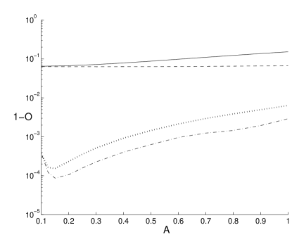
Figure 3: Overlaps of the approximate wave-functions with the exact one, as a function of the adiabaticity parameter, for $SA=2$. The value $1-O=0$ correspond to perfect agreement. The full line is the adiabatic approximation, the dashed line is the pseudo-adiabatic approximation, the dotted line is the coherent state approximation and the dot-dashed line is the symmetrized approximation

So, we see from these approximations that a crucial feature of them is the fact that the most relevant terms in the evolution operator conserve the spin projection along the local direction of the magnetic field. This is the basis of the semi-classical calculation performed in prasara , in which the states with definite spin projections along the local magnetic field were taken as coherent internal states, and hence their motion could be described in terms of trajectories.

Despite the fact that the approximations discussed here, specially the coherent state and symmetrized approximations, are very accurate, they do not describe an important effect of the exact evolution operator. In all the approaches described here, the scattering amplitudes for given spin projections along the y-axis (the beam axis), are equal, up to a phase factors, to the amplitudes in which the spin projections are reversed. This is a result of the fact that only terms which commute with $I_{B}$ are allowed in the expansion of the evolution operator.

V Revisiting Stern-Gerlach experiments

In the text book description of the Stern-Gerlach experiment, the deflection of the beam gives information of the spin projection along the $z-$axis, which is the one that points along the magnetic field at the centre of the beam. The deflection of the beam is not sensitive to the spin components along other directions. If, for a spin-1/2 particle, the initial spin points along the $x-$axis, $m_{x}=+1/2$, the text book description would indicate that the pattern of scattered particles would be completely equivalent to that one produced by a mixture of 50% $m_{z}=+1/2$ and 50% $m_{z}=-1/2$ particles. The same would be true for $m_{x}=-1/2$. So, a Stern-Gerlach experiment is not expected to give any asymmetry between different spin projections perpendicular to the z-axis.

To investigate this question, we define the asymmetry for a given axis as the difference in the probabilities of finding the scattered particles in a given position in the $(z,x)$ plane, for the two spin projections. Thus, we have

$$A_{z}(x,z) = \sum_{mm_{0}m_{0}^{\prime}}\langle x,z;m|\Phi(t);m_{0}\rangle\langle x,z;m|\Phi(t);m_{0}^{\prime}\rangle^{*}\langle m_{0}|\sigma_{z}|m_{0}^{\prime}\rangle$$ (37)

$$A_{x}(x,z) = \sum_{mm_{0}m_{0}^{\prime}}\langle x,z;m|\Phi(t);m_{0}\rangle\langle x,z;m|\Phi(t);m_{0}^{\prime}\rangle^{*}\langle m_{0}|\sigma_{x}|m_{0}^{\prime}\rangle$$ (38)

$$A_{y}(x,z) = \sum_{mm_{0}m_{0}^{\prime}}\langle x,z;m|\Phi(t);m_{0}\rangle\langle x,z;m|\Phi(t);m_{0}^{\prime}\rangle^{*}\langle m_{0}|\sigma_{y}|m_{0}^{\prime}\rangle$$ (39)

Note that, in the standard description of the Stern Gerlach experiment, the spin projection along the $z$ axis is conserved, and thus the asymmetries $A_{x}$ and $A_{y}$ should vanish at all points. This is not the case. As shown in figure 4b, there is a difference in the pattern of particles scattered depending on the spin projection along the $x$-axis. This effect is found to depend on the inhomogeneity of the magnetic field, which is determined by $z_{0}=B_{0}/B_{1}\sigma$. If $z_{0}$ is large, the inhomogeneity of the magnetic field explored by the beam is small, and so is $A_{x}$. This asymmetry can be calculated, with various degrees of accuracy, making use of the approximate treatments discussed here. It can also be calculated with the semi-classical treatment of prasara . The origin of this asymmetry can be understood by arguing that, the motion in an inhomogeneous magnetic field conserves the spin projection along the local magnetic field, which has a different direction for the different parts of the wave-function. This links with the concept of coherent internal states, which were introduced in sara .

The calculations in figure 4a show also that there is an asymmetry $A_{y}$ which means that there is a dependence of the spin projection along the y-axis. This is a dynamical effect, which does not appear in the semi-classical description. In fact, the analytic approximations presented here, the value of $A_{y}$ vanishes after the interaction. Only after allowing for some time of free evolution, non-vanishing values of $A_{y}$ develop. The origin of this asymmetry arises from the term $AS^{2}p_{\beta}I_{y}$ which appears in the double commutator $[[h_{0},v],v]$. The effect of this term can be understood because $p_{\beta}$ is the generator of rotations in the $(x,z)$ plane, around the point $x=0,z=-z_{0}$ where the field vanishes. The effect of this term in the expansion of the evolution operator, would generate a rotation in the wave-function, around the point where the field vanishes, which will be opposite for the different spin projections along the z-axis. Indeed, this effect competes with the interaction $v=S\rho I_{B}$, which tends to preserve the spin projection along the direction of the field. The result of this competition is that the magnitude of the asymmetry depends on the ratio $AS/z_{0}$.

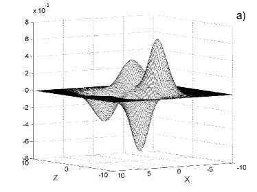
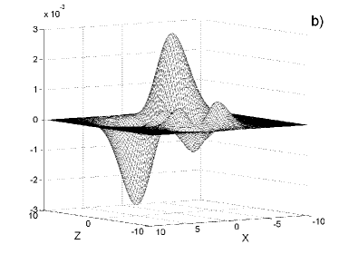
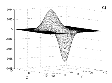
Figure 4: Asymmetries for particles polarised along the $y$ (a), $x$ (b), and $z$ (c) directions. Note that the maximum asymmetry occurs for particles polarised along the z-axis, but that there are important asymmetries for particles polarised along the x-axis and the y-axis.

The fact that all the asymmetries are non-vanishing, and also that they have different behaviour as a function of $(x,z)$, leads to an exciting possibility. Consider that we have a beam of particles, so that we do not know their polarisation state. We can make the beam go through an inhomogeneous field, as described here, and detect the pattern of scattered particles. Let the polarisation state be described initially as a density matrix $\rho=1/2(I+p_{x}\sigma_{x}+p_{y}\sigma_{y}+p_{z}\sigma_{z})$, where $\vec{p}$ is a vector which measures the degree and direction of the beam polarisation. Then, the density of particles detected in the $(x,z)$ plane will be proportional to

$$P(x,z)=P_{0}(x,z)+{1\over 2}(p_{x}A_{x}(x,z)+p_{y}A_{y}(x,z)+p_{z}A_{z}(x,z))$$ (40)

This allows to obtain all the components of the polarisation vector from the pattern of scattered particles, when a sufficient number of particles are detected. Note that, in contrast to expression 40, the text-book description of The Stern-Gerlach experiment would be consistent with a probability density given by

$$P(x,z) = P_{0}(x,z)+{1\over 2}p_{z}A_{z}(x,z)$$ (41)

$$A_{z}(x,z) = 2P_{0}(x,z)\quad z>0$$

$$A_{z}(x,z) = -2P_{0}(x,z)\quad z<0$$

This expression, when applicable, would allow to obtain information only on the value of $p_{z}$.

VI Summary and conclusions

We have investigated the motion of a particle with spin in an inhomogeneous magnetic field using a quantum mechanical framework. Our aim is to investigate in detail the limitations of the usual textbook approach to Stern-Gerlach experiments, that assumes that the spin projection along the direction of the magnetic field is conserved, while different spin components acquire a momentum which depends on the gradient of the field.

We find that, consistently with a previous semi-classical analysis, there is a sizeable probability of spin flip, which depends on the inhomogeneity of the field. Besides, there is a focusing effect in the component that deviates towards in the direction in which the modulus of the field decreases. These characteristics are very robust, and occur in dynamical situations which are far from the semi-classical limit.

Thus, we can conclude that the Stern-Gerlach experiment is not, even in principle, and ideal experiment, which would “project” the internal state into the eigenvalues of the measurement operator. Moreover, the experiment is not fully reliable, as the position or momenta of the particles do not give unequivocal information on the spin projection. The magnitude that determines how close is a Stern-Gerlach experiment to an ideal reliable measurement is $z_{0}=\sigma B_{0}/B_{1}$. Only when the magnetic field $B_{0}$ is very large compared to its gradient, or when the size of the beam $\sigma$ is very small, the Stern-Gerlach experiment would approximate to an ideal reliable measurement.

We have investigated different approximate treatments of the exact quantum-mechanical problem. We find that, to a good approximation, the interaction occurs as if the spin projection along the magnetic field at each position was conserved. This indicates that, for each position in the inhomogeneous field, the states with given spin projection along the magnetic field are coherent internal states. Then, provided that the quantum size of the wave-function is small compared to the inhomogeneity of the magnetic field, it is meaningful to approximate the motion of these states in terms of classical trajectories. This justifies the treatment performed in prasara .

It is interesting to note that the adiabatic approximation it is not accurate, even in the limit of small $A$ (large mass, or short interaction time), if, at the same time, the interaction is large so that it generates a fixed deflection angle. This observation can be relevant to cases, such as in nuclear physics ron , in which although the collision times are short to guarantee the validity of the adiabatic approximation, the forces are so strong to produce a finite deflection.

Our calculations indicate that the Stern-Gerlach experiment is not an ideal measuring apparatus, in the sense of neumann . However, this does not mean that one cannot acquire an accurate knowledge from the spin state of the projectile by observing the statistical results of the experiment. On the contrary: while an idealised Stern-Gerlach experiment will not give any information of the spin projection along the $x$ or $y$ axis, the analysis of a realistic Stern-Gerlach experiment, such as modelled in our calculations, can give the value of all the components of the density matrix that describes the polarisation of the beam.

Our analysis supports the idea that the interpretation of realistic experiments does not require the use of the reduction principle, as discussed by several authors in reduc . Thus, the interaction between the spin and the magnetic field, which is described in a purely quantum mechanical framework, generates a correlation between the spin polarisation of the beam and the final position of the particles of the beam. A measurement of a sufficiently large number of these positions, allows to determine the components of the density matrix of the beam with sufficient statistical accuracy. The reduction principle is not required in this argument.

- (1) R. Eisberg and R. Resnick, Quantum Physics, Wiley, 1974.
- (2) J.M. Levy-Leblond and F. Balibar, Quantics, North Holland, 1990.
- (3) E. Merzbacher, Quantum Mechanics, Wiley, 1998.
- (4) A. Messiah, Mechanique Quantique, Dunod, 1965.
- (5) J. von Neumann, Mathematical Foundations of Quantum Mechanics, Princeton University Press (1955).
- (6) A. Bassi and G. Ghirardi, Physics Letters A 275 (2000) 373-381.
- (7) S. Cruz-Barrios and J. Gómez-Camacho, Phys. Rev. A63 (2000) 012101
- (8) S. Cruz-Barrios and J. Gómez-Camacho, Nucl. Phys. A636 (1998) 70-84
- (9) B. M. Garraway and S. Stenholm, Phys. Rev. A60 (1999) 63-79
- (10) H. M. Fran a, T. W. Marshall, E. Santos and E.J. Watson, Phys. Rev. A46 (1992) 2265-2270.
- (11) M. Cini and J-M. L vy-Leblond (Editors). “Quantum Theory Without Reduction.” Adam Hilguer, Bristol, 1990.
- (12) R.C. Johnson, “Scattering and reactions of halo nuclei”, in “An advanced course in modern nuclear physics”, Eds. JM Arias and M Lozano, Springer-Verlag, 2001, pp259-291.