Abstract

It is shown that the Kapitza-Dirac effect with atoms, which has been considered to be evidence for their wavelike character, can be interpreted as a scattering of pointlike objects by the periodic laser field.

1 Introduction

The currently accepted answer to the question posed in my title is, of course, ”Both”. But I submit that we should not abandon the heritage passed down to us by the Atomists, from Democritus to Boltzmann. It was a long struggle, at times involving scientific isolation and consequent personal suffering[1], to establish the atomicity of matter (from which I exclude radiation for present purposes).

In recent times some  experimental evidence has been found to support a wavelike description of atoms, and even of quite large molecules such as fullerene. I shall concentrate here on the first category, in which something analogous to the diffraction of light has been observed with a ”monochromatic” beam of atoms, the grating being supplied by a stationary laser wave which is tuned to a frequency close to an atomic resonance[2]. Actually it is not so much the monochrome property which is important – the velocity of the beam was controlled only to within about 5% of its mean value – but rather a very high degree of collimation – the component of momentum perpendicular to the laser must be an order of magnitude less than $h/\lambda$, where $h$ is Planck’s constant and $\lambda$ is the laser wave length. For sodium atoms with a mean velocity of 10³ms^-1, and with the laser tuned to the D-line at 589nm, this demands an initial angular spread less than 3.10^-5radians. What we observe in the outgoing beam is a set of well separated peaks at integral multiples of 6.10^-5rad. There is a well worked out theory of the broadening of these lines[3][4], but the spacing of $2h/\lambda Mv$, as well as the intensities, may be explained with a very simple quantum mechanical (QM) model to be outlined in the next section. This model was discussed by Gould[2], who offered two interpretations of the analysis; we must accept either that each atom is spread out over a wave front of the order of several microns or that the atom trades in quanta of momentum. The first alternative is the description given long ago by Kapitza and Dirac[5] of a diffraction process in which an atomic wave whose wavelength is $h/Mv$ is diffracted by a grating whose spacing is $\lambda/2$, while the second views the process as one of scattering in which the atom absorbs and emits, stochastically, radiation from and to the laser field in quanta of $hc/\lambda$; such radiation is in one of the two (up or down) directions of the laser beam, and so its Poynting vector carries a transverse momentum of $\pm h/\lambda$, and this must be compared with a longitudinal momentum of $Mv.$ But, curiously, the latter analysis indicates that events of emission and absorption occur in pairs, so that very few atoms emerge from the laser having a transverse momentum which is an odd multiple of $h/\lambda$.

Gould did not choose to emphasize the contradictory nature of these two interpretations; he instead pointed out that either of them were ”equally unpalatable to the prequantum physicist”. Staying within the Atomist tradition I propose to reject the first interpretation and accept the second. Nevertheless, I enter the reservation that I can do so staying largely within a classical (or prequantum) world view. There is a fair amount of evidence[6] that Max Planck, who discovered the quantum discontinuity in absorption and emission of light, never accepted that the light field itself had to be quantized. A quotation from a letter to Einstein in 1907 illustrates Planck’s view of the light field.

I am not seeking the meaning of the quantum of action (light quantum) in the vacuum but rather in places where emission and absorption occur, and I assume that what happens in the vacuum is rigorously described by Maxwell’s equations.

In summary, I propose, from Section 3 onwards, to investigate whether the distribution pattern of the scattered atoms may be explained on the basis of a model in which quanta $h/\lambda$ of momentum are exchanged, stochastically, with the laser field. Before that I shall summarize, in Section 2, the results of the simplified QM theory, which will provide us with a standard for comparison.

2 The QM model

The hamiltonian is

$$H\left(t\right)=\frac{1}{2}\hbar\left(\omega-\Delta\right)\sigma_{3}+\hbar\Omega_{R}\cos\zeta\left(\sigma_{1}\cos\omega t+\sigma_{2}\sin\omega t\right)\text{ },\text{ }0<t<t_{0}\text{ ,}$$ (1)

where $\omega$ is the laser frequency, detuned by $\Delta$ from the D-line resonance $\omega_{0}$, $\Omega_{R}$ is the resonant Rabi frequency of the interaction, and $\sigma_{1},\sigma_{2},\sigma_{3}$ are the Pauli spin matrices interpreted, in the standard manner, as atomic raising and lowering operators. The kinetic energy $\left(h^{2}/2M\lambda^{2}\right)\left(\partial^{2}/\partial\zeta^{2}\right)$ has been discarded on account of the large atomic mass $M,$ and the variable $\zeta,$ which takes values in the range $\left(-\pi/2,\pi/2\right)$ (see Fig.1),

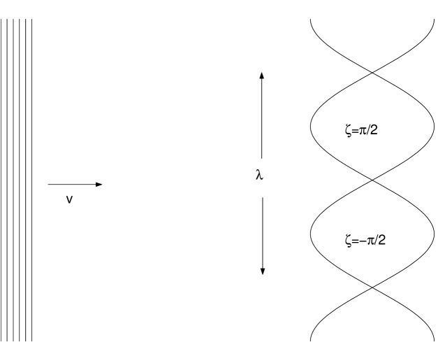
Figure 1: The Kapitza-Dirac effect according to the QM model, which is the original description of Dirac and Kapitza. A de Broglie wave, whose wavelength is small, and whose coherence width is large, compared with $\lambda$, is incident on a stationary laser of wavelength $\lambda$. The de Broglie wave experiences the laser as a sinusoidally varying refractive index with spacing $\lambda/2$, and emerges as a diffraction pattern whose maxima are separated by angular intervals of $2h/\lambda Mv$ radians.

gives the phase of the atom in the laser wave at the point of entry. On account of the assumption of infinite mass, this is also the phase at the point of exit. Starting from an initial state having zero transverse momentum and in the lower state of the D-line couplet, that is

$$\psi\left(0;\zeta\right)=\left(\begin{array}[]{c}0\\ 1\end{array}\right)\text{ ,}$$ (2)

the state at time $t_{0}$ is

$$\left(\begin{array}[]{c}\psi_{u}\left(t_{0};\zeta\right)e^{i\omega t_{0}/2}\\ \psi_{l}\left(t_{0};\zeta\right)e^{-i\omega t_{0}/2}\end{array}\right)=\left(\begin{array}[]{c}\left[-i(\Omega_{R}/\Omega)\cos\zeta\sin\Omega t_{0}\right]e^{i\omega t_{0}/2}\\ \left[\cos\Omega t_{0}+i\left(\Delta/2\Omega\right)\sin\Omega t_{0}\right]e^{-i\omega t_{0}/2}\end{array}\right)\text{ ,}$$ (3)

where $\Omega=\sqrt{\left(\Delta^{2}/4\right)+\Omega_{R}^{2}\cos^{2}\zeta}$. The amplitudes $\psi_{u}$ and $\psi_{l}$ are the parts of the wave function representing an atom in its upper and lower state respectively. In order to observe the discrete momentum spectrum it was found necessary to make $\Delta$ substantially larger than $\Omega_{R};$ typically $\Delta\approx 5\Omega_{R}$. We therefore expand the wave function in powers of $\gamma=\Omega_{R}/\Delta$ giving, to order $\gamma^{2}$,

$$\psi_{u}\left(t_{0};\zeta\right) = -2i\gamma\cos\zeta\sin\Omega^{\prime}\tau\text{ ,}$$

$$\psi_{l}\left(t_{0};\zeta\right) = e^{i\Omega^{\prime}\tau}-2i\gamma^{2}\cos^{2}\zeta\sin\Omega^{\prime}\tau\text{ ,}$$ (4)

where

$$\tau=t_{0}\gamma^{2}\Delta/2\qquad,\qquad\Omega^{\prime}=\gamma^{-2}+1+\cos 2\zeta\text{ .}$$ (5)

The Fourier series for the transition amplitude is then

$$\psi_{u}\left(\tau;\zeta\right)=-i\gamma\sum_{n=-\infty}^{\infty}\left[J_{n}\left(\tau\right)\sin\tau_{n}+J_{n+1}\left(\tau\right)\cos\tau_{n}\right]e^{\left(2n+1\right)i\zeta}\text{ ,}$$ (6)

where

$$\tau_{n}=\frac{\left(1+\gamma^{2}\right)\tau}{\gamma^{2}}+\frac{n\pi}{2}\text{ ,}$$ (7)

and for the no-transition amplitude it is

$$\psi_{l}\left(\tau;\zeta\right)=\sum_{-\infty}^{\infty}e^{2in\zeta}\left[e^{i\tau_{n}}J_{n}\left(\tau\right)-i\gamma^{2}\{J_{n}\left(\tau\right)\sin\tau_{n}-J_{n}^{\prime}\left(\tau\right)\cos\tau_{n}\}\right]\text{ .}$$ (8)

The lower component gives the intensities of the even lines of the spectrum, namely

$$\rho_{n}^{\text{Q}}\left(\tau\right)=J_{n}^{2}\left(\tau\right)\left(1-2\gamma^{2}\sin^{2}\tau_{n}\right)+\gamma^{2}J_{n}\left(\tau\right)J_{n}^{\prime}\left(\tau\right)\sin 2\tau_{n}\text{ ,}$$ (9)

while the upper component gives the odd lines, namely

$$\rho_{n+1/2}^{\text{Q}}\left(\tau\right)=\gamma^{2}\left[J_{n}\left(\tau\right)\sin\tau_{n}+J_{n+1}\left(\tau\right)\cos\tau_{n}\right]^{2}\text{ .}$$ (10)

The wave interpretation of Kapitza and Dirac is made by considering the limit $\gamma\rightarrow 0$, so that the outgoing wave function is effectively the scalar

$$\psi\left(t_{0};\zeta\right)=\exp\left[i\left(-\frac{1}{2}\omega_{0}t_{0}+2\tau\cos^{2}\zeta\right)\right]\text{ .}$$ (11)

The dependence of $\psi$ on $\zeta$ is an indication (see Fig.1) that the de Broglie wave of the atom experiences a spatially varying refractive index as it goes through the laser, and its Fourier expansion, that is

$$\exp\left(2i\tau\cos^{2}\zeta\right)=\sum_{n=-\infty}^{\infty}i^{n}e^{i\tau}J_{n}\left(\tau\right)e^{2in\zeta}\text{ ,}$$ (12)

indicates that the atom acquires a transverse momentum of either $2nh/\lambda$ or $-2nh/\lambda$ with probability

$$\rho_{n}^{\text{Q}0}\left(\tau\right)=J_{n}^{2}\left(\tau\right)\text{ ,}$$ (13)

for which the characteristic function is

$$F_{\text{Q}0}\left(\theta;\tau\right)=\left\langle e^{in\theta}\right\rangle=\sum_{n=-\infty}^{\infty}J_{n}^{2}\left(\tau\right)e^{in\theta}=J_{0}\left(2\tau\sin\frac{\theta}{2}\right)\text{ .}$$ (14)

The moments of the distribution are obtained from the derivatives of $F$. In particular the variance is

$$\left\langle n^{2}\right\rangle_{\text{Q}0}=\sum_{n=-\infty}^{\infty}n^{2}J_{n}^{2}\left(\tau\right)=-F_{\text{Q}0}^{\prime\prime}\left(0;\tau\right)=\frac{1}{2}\tau^{2}\text{ .}$$ (15)

This has the form, for small $\tau,$

$$\left\langle n^{2}\right\rangle_{\text{Q}0}=2\rho_{1}^{\text{Q}0}\left(\tau\right)+O\left(\tau^{4}\right)\text{ ,}$$ (16)

which establishes that changes in $n$ occur in single steps of $\pm 1$.

We shall need to consider the asymptotic behaviour as $\tau\rightarrow\infty$ of this spectrum, namely[8]

$$\rho_{n}^{\text{Q}0}\left(\tau\right)\sim\left\{\begin{array}[]{c}2\pi^{-1}\left(\tau^{2}-n^{2}\right)^{-1/2}\cos^{2}\left[\sqrt{\tau^{2}-n^{2}}-\beta|n|-\pi/4\right]\quad\left(|n|<\tau\right)\text{ ,}\\ 0\qquad\qquad\qquad\qquad\qquad\qquad\left(|n|>\tau\right)\text{ ,}\end{array}\right.$$ (17)

where

$$\beta=\cos^{-1}\left(|n|/\tau\right)\text{ .}$$ (18)

These intensities oscillate, with angular frequency $1/2$ for small $n$, but decreasing as $n$ approaches $\tau$.

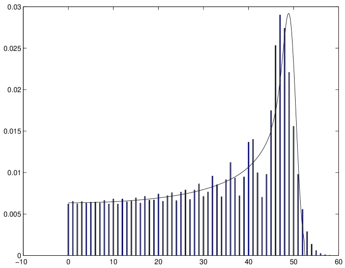
Figure 2: The momentum spectrum, averaged over the velocity profile, of the Kapitza-Dirac effect according to the QM model, with the time parameter $\tau=50$. The bar chart represents the intensity of the $n$th line and the continuous curve depicts a deterministic classical model. Since the observed datum is actually the angular deflection, the experimental method used cannot distinguish the two spectra at this value of $\tau$.

However, the oscillations disappear once we take account of the beam’s velocity profile, described by a gaussian function $H(\tau)$, with standard deviation $\sigma=$0.025$\tau$, so that 95% of the atoms have transit times within 5% of the mean. The averaged intensities are

$$\overline{\rho_{n}^{\text{Q}0}}\left(\tau\right)=\int_{0}^{\infty}J_{n}^{2}\left(\tau^{\prime}\right)H\left(\tau,\tau^{\prime}\right)d\tau^{\prime}\sim\frac{1}{\pi\sigma\sqrt{2\pi}}\int_{n}^{\infty}\exp\left[-\frac{\left(\tau-\tau^{\prime}\right)^{2}}{2\sigma^{2}}\right]\frac{d\tau^{\prime}}{\sqrt{\tau^{\prime 2}-n^{2}}}\text{ ,}$$ (19)

I have plotted, in Fig.2, the values of $\overline{\rho_{n}^{\text{Q}0}}$ and its asymptotic limit at $\tau=50$. The latter curve actually coincides with a completely classical model of the process, in which an atom going through the laser at phase $\zeta$ acquires a momentum of $\tau\sin 2\zeta,$ and $\zeta$ has uniform density between $-\pi/2$ and $\pi/2$. For such large $\tau$ it is this classical curve which would be observed, because the experimental datum is the angular deflection, rather than the transverse momentum, of the atom; the individual lines of the spectrum are broadened, so that they merge with one another.

The exact spectrum, given by (9) and (10), displays rapid oscillations because of the sinusoidal terms in $\tau_{n}$, in addition to the slower oscillations we have just been considering. But, except in a short initial period, the rapid oscillations disappear for all $n$ after smoothing with $H$.

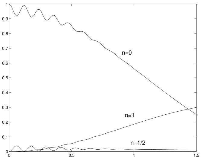
Figure 3: The intensities of the first few lines, averaged over the velocity profile, in the QM model for small values of the transit time $\tau$. The parameter $\gamma$ has been set at 0.2.

I have plotted the smoothed spectrum for the first few values of $n$ in Fig.3; with $\gamma=0.2$ the rapid oscillations are effectively damped out for $\tau>1$. For the actual experimental range of $2<\tau<6,$ we may smooth by putting simply $\left\langle 2\sin^{2}\tau_{n}\right\rangle=\left\langle 2\cos^{2}\tau_{n}\right\rangle=1$ and $\left\langle\sin 2\tau_{n}\right\rangle=0$, leading to

$$\overline{\rho_{n}^{\text{Q}}}\left(\tau\right)=J_{n}^{2}\left(\tau\right)\left(1-\gamma^{2}\right)\text{ , }\overline{\rho_{n+1/2}^{\text{Q}}}\left(\tau\right)=\frac{\gamma^{2}}{2}\left[J_{n}^{2}\left(\tau\right)+J_{n+1}^{2}\left(\tau\right)\right]\text{ ,}$$ (20)

and this corresponds to the characteristic function

$$F_{\text{Q}}\left(\theta;\tau\right)=F_{\text{Q}0}\left(\theta;\tau\right)\left[1+\gamma^{2}\left(\cos\frac{\theta}{2}-1\right)\right]\text{ .}$$ (21)

3 A stochastic model

In his article, Gould[2] states that ”…if we attempt to assign specific points in the diffraction pattern to specific locations in the standing wave, we will fail miserably”. While not dissenting from this judgement, I stress that many areas of classical physics produce situations of the same character; if we were to try to predict the position of a Brownian particle given its initial position and momentum, then we would fail equally miserably. What probably motivated the statement is the Heisenberg Inequality as applied to an atom of the beam. Since its transverse momentum is defined by the collimation process to be a small fraction of $h/\lambda$, its position ”uncertainty” is a large multiple of $\lambda$; this is reflected in our choice of initial wave function $\psi\left(0;\zeta\right)=1$ in the previous section, giving uniform probability for all $\zeta$. However, the maximum deflection, in a typical case where four even lines are visible either side of the central line and the transverse momentum at entrance to the beam is zero, is 2.4.10^-4rad, so, for a laser of width 0.1mm, the maximum change in the value of $\zeta$ at exit is 24nm or 0.04$\lambda$. Although the observed variable is the momentum, which means that $\zeta$, in QM parlance, is a ”hidden” variable, I assert that it is not unreasonable to maintain that, to within the atomic diameter, somewhat less than 1nm, each atom in the beam has a well defined $\zeta$, which varies only slightly as the atom crosses the laser. For the moment I shall confine the model to the case $\gamma\rightarrow 0,$ which means we are assuming the upper internal state of the atom is infinitely short lived and only even lines of the momentum spectrum are seen.

The model I propose is that of a Markov process on the set of integers $n\left(\tau;\zeta\right)$, the transition matrix being $\lambda_{mn}\left(\zeta\right)$, that is the probability of a transition from $n$ to $m$ in an interval $\delta\tau$ is $\lambda_{mn}\left(\zeta\right)\delta\tau+o\left(\delta\tau\right)$. The Markov property means we assume that transitions in successive intervals occur independently. I shall make two further assumptions: (i) the process is single-step, so $\lambda_{mn}=0$ unless $m=n\pm 1;$ this is suggested by the property (16) of the QM process (ii) the process is homogeneous, and therefore[7] additive, so $\lambda_{m+r,n+r}=\lambda_{mn}$. With these assumptions, the transition matrix has only two independent components, denoted $\lambda_{n+1,n}=\alpha\left(\zeta\right)$ and $\lambda_{n-1,n}=\beta\left(\zeta\right)$.

To summarize, the stochastic model of the process associates, with a specific location $\zeta$ in the standing wave, a specific Markov process with the parameters $\alpha\left(\zeta\right),\beta\left(\zeta\right)$.

The characteristic function for $n\left(\tau;\zeta\right)$ is

$$f_{\text{S}}\left(\theta;\tau;\zeta\right)=\left\langle e^{in\theta}\right\rangle=\exp\left[\tau\alpha\left(\zeta\right)\left(e^{i\theta}-1\right)+\tau\beta\left(\zeta\right)\left(e^{-i\theta}-1\right)\right]\text{ ,}$$ (22)

and its occupation probabilities are

$$P_{n}\left(\tau;\zeta\right)=\left(\frac{\alpha}{\beta}\right)^{n/2}\exp\left[-\alpha\tau-\beta\tau\right]I_{n}\left(2\tau\sqrt{\alpha\beta}\right)\text{ .}$$ (23)

The predicted line intensities are obtained by integrating over the ”hidden” variable $\zeta$, that is

$$\rho_{n}^{\text{S}}\left(\tau\right)=\frac{1}{\pi}\int_{-\pi/2}^{\pi/2}P_{n}\left(\tau;\zeta\right)d\zeta\text{ ,}$$ (24)

where $P_{n}\left(\tau;\zeta\right)=P_{n}\left(\tau;\zeta+\pi\right).$ I shall assume further that $\alpha\left(\zeta+\pi/2\right)=\beta\left(\zeta\right)$, which results in

$$P_{n}\left(\tau;\zeta\right)=P_{-n}\left(\tau;\zeta+\pi/2\right)\text{ ,}$$ (25)

and hence

$$\rho_{n}^{\text{S}}\left(\tau\right)=\rho_{-n}^{\text{S}}\left(\tau\right)=\frac{2}{\pi}\int_{0}^{\pi/2}P_{n}\left(\tau;\zeta\right)d\zeta\text{ .}$$ (26)

A concrete example of such a model is

$$\alpha\left(\zeta\right)=\frac{1+\sin 2\zeta}{2}\quad,\quad\beta\left(\zeta\right)=\frac{1-\sin 2\zeta}{2}\text{ .}$$ (27)

This model is depicted in Fig.4,

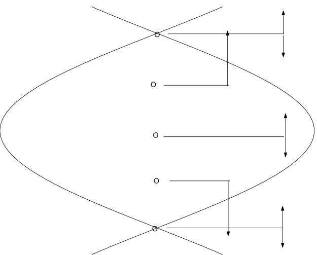
Figure 4: The Kapitza-Dirac effect according to the stochastic model. For a given location of the atom in the stationary wave, there is a pair of transition probabilities, for transverse impulses of $\pm 2h/\lambda$ respectively. The sum of these probabilities is the same for all locations. For example, the two probabilities are equal at a node or an antinode, while one of them is zero at a point midway between a node and an antinode; the atom moves preferentially towards the nearest node.

where the directions and magnitudes of the transition rates $\alpha\left(\zeta\right),\beta\left(\zeta\right)$ are indicated for a few different locations of the atom within the standing wave. Putting $\xi=\zeta-\pi/4$, the intensities become

$$\rho_{n}^{\text{S}}\left(\tau\right) = \frac{2e^{-\tau}}{\pi}\int_{0}^{\pi/2}\tan^{n}\xi\text{ }I_{n}\left(\tau\sin 2\xi\right)d\xi$$ (28)

$$= \frac{e^{-\tau}}{\pi}\sum_{r=0}^{\infty}\frac{\Gamma\left(r+1/2\right)\Gamma\left(n+r+1/2\right)}{r!\left(n+r\right)!\left(n+2r\right)!}\text{ }\tau^{n+2r}\text{ ,}$$

and the characteristic function is (compare eqn(7))

$$F_{\text{S}}\left(\theta;\tau\right)=\sum_{n=-\infty}^{\infty}\rho_{n}^{\text{S}}\left(\tau\right)e^{in\theta}=\exp\left[-\tau\left(1-\cos\theta\right)\right]J_{0}\left(\tau\sin\theta\right)\text{ .}$$ (29)

4 Comparison of the models

The latter model has a variance

$$\left\langle n^{2}\right\rangle_{\text{S}}=\frac{1}{2}\tau^{2}+\tau\text{ ,}$$ (30)

as compared with the QM variance of $\tau^{2}/2$. Whilst the variances become indistinguishable for large $\tau$, for small $\tau$ there is an essential difference; the initial variance is of order $\tau^{2}$ in the QM model, and of order $\tau$ in the stochastic model. I postpone discussion of this disagreement to the Discussion section.

In making a more detailed examination of the spectrum we begin by comparing the asymptotics of the QM and stochastic models in the limit $\tau\rightarrow+\infty.$ The QM intensities were obtained in Section 2, and we now compare them with the asymptotics of the stochastic model, which are obtained from its characteristic function

$$G_{\text{S}}\left(\tau;z\right)=\frac{1}{\pi}\int_{-\pi/2}^{\pi/2}\exp\left[\frac{1}{2}z\left(1+\sin 2\zeta\right)+\frac{1}{2}z^{-1}\left(1-\sin 2\zeta\right)-1\right]d\zeta\text{ ,}$$ (31)

namely

$$\rho_{n}^{\text{S}}\left(\tau\right)=\frac{1}{2\pi i}\int_{C}G_{\text{S}}\left(\tau;z\right)z^{-n-1}dz\text{ ,}$$ (32)

where $C$ is a closed contour enclosing the origin. This set of functions has the surprisingly simple asymptotic behaviour (obtained by selecting a steepest-descent contour for $C$)

$$\rho_{n}^{\text{S}}\left(\tau\right)\sim\frac{1}{\pi\sqrt{\tau^{2}-n^{2}}}\qquad\left(|n|<\tau\right)\text{ ,}$$ (33)

which, on averaging over the velocities of the atomic beam, gives exactly the same asymptotics as the QM model, that is (see Fig.2)

$$\overline{\rho_{n}^{\text{S}}}\left(\tau\right)=\int_{0}^{\infty}\rho_{n}^{\text{S}}\left(\tau^{\prime}\right)H\left(\tau,\tau^{\prime}\right)d\tau^{\prime}\sim\overline{\rho_{n}^{\text{Q}0}}\left(\tau\right)\text{ .}$$ (34)

Now, turning to small values of $\tau$, I  plot, in Fig.5,

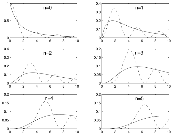
Figure 5: The momentum spectrum of the Kapitza-Dirac effect according to the stochastic model. The continuous lines represent the intensity of the $n$th line as a function of the time $\tau$ spent in the laser, and the dashed line represents the equivalent intensity in the QM model. At $\tau=3$ only the lines $n\leq 4$ are visible.

the unsmoothed intensities, that is $\rho_{n}^{\text{Q}0}$ and $\rho_{n}^{\text{S}},$ of the first six lines as functions of $\tau$. Note that the QM and the stochastic models agree as to their orders of magnitude; in particular the latter model gives just four visible lines on either side of the centre line for the case $\tau=3$. However, these curves show the disagreement of variances noted above; it shows up as a zero slope at the origin for all $\rho_{n}^{\text{Q}0}$, compared with a negative slope for $\rho_{0}^{\text{S}}$ and a positive slope for $\rho_{1}^{\text{S}}$; the zero slope for higher $\rho_{n}^{\text{S}}$ is a consequence of the single-step assumption which we made in constructing the stochastic model.

A more serious disagreement is the oscillatory dependence of $\rho_{n}$ on $\tau$ in the QM model. Indeed that model predicts zero intensity for $\rho_{n}\left(\tau\right)$ whenever $J_{n}\left(\tau\right)$ has a zero. An averaging over $\tau,$ as above, will give a smoothed intensity which never completely vanishes, but nevertheless, for small $\tau$, the oscillations persist even with such smoothing. On the other hand, in our concrete stochastic model $\rho_{0}$ decreases monotonically, while the other $\rho_{n}$ rise to a single maximum and then decrease monotonically, that is there are no zeros. This behaviour is common to the whole family of Markov models, as may be seen by considering the derivative

$$\frac{\partial}{\partial\tau}\left[\tau^{-n}e^{-\alpha\tau-\beta\tau}I_{n}\left(2\tau\sqrt{\alpha\beta}\right)\right]=-\tau^{-n}e^{-\alpha\tau-\beta\tau}\left[\left(\alpha+\beta\right)I_{n}-2\sqrt{\alpha\beta}I_{n+1}\right]\text{ .}$$ (35)

The right hand side is negative for all positive $\alpha,\beta,\tau$ and all nonnegative $n$, and therefore, substituting in (24),

$$\frac{d}{d\tau}\left[\tau^{-n}\rho_{n}^{\text{S}}\left(\tau\right)\right]<0\qquad\qquad\left(n\geq 0,\tau>0\right)\text{ .}$$ (36a)

Thus $$\rho_{0}^{\text{S}}\left(\tau\right) \overline{\rho_{0}^{\text{S}}}\left(\tau\right) \rho_{0}^{\text{Q}}\left(\tau\right) \overline{\rho_{0}^{\text{Q}}}\left(\tau\right) n>0 \rho_{n}^{\text{Q}}\left(\tau\right)$$ certainly decreases monotonically, as does also but not or . For the implication of the inequality is somewhat more complicated, but it is certainly not satisfied by .

5 Inclusion of odd-momentum states

I shall now improve the model by including the odd states, so that $n$ takes half-integral as well as integral values. A jump of $\pm 1/2$ from an even (that is integral $n$) state occurs with probability $\delta\tau$, that is either direction is equally probable, and a jump of $+1/2$ from an odd state occurs with probability $\delta\tau\left(1+\sin 2\zeta\right)/\gamma^{2}$, while a jump of $-1/2$ from an odd state occurs with probability $\delta\tau\left(1-\sin 2\zeta\right)/\gamma^{2}$. Adopting the standard classification of stochastic processes, the new model may be described as a pair of coupled additive processes, an additive process[7] being one which is homogeneous and Markov. Because of the factors of $\gamma^{-2}$, this model gives a correction to $F_{\text{S}0}$ even to zero order, but we shall see that such corrections are substantial only for $\tau$ of order $\gamma^{2}$. Outside of this range, the corrections to $F_{\text{S}0}$ are of order $\gamma^{2}$ only, so they do not significantly reduce the disagreements we have just found between $\rho_{n}^{\text{S}}$ and $\rho_{n}^{\text{Q}}$.

The characteristic function for the new model is

$$F_{\text{S}}\left(\theta;\tau\right)=\frac{1}{\pi}\int_{-\pi/2}^{\pi/2}f_{\text{S}}\left(\theta;\tau;\zeta\right)d\zeta\text{ ,}$$ (37)

where the function $f_{\text{S}}\left(\theta;\tau;\zeta\right)$ may be decomposed into parts coming from even and odd states, that is

$$f_{\text{S}}=f_{1}+f_{2}\text{ , }f_{1}=\sum_{-\infty}^{\infty}P_{n}\left(\tau;\zeta\right)e^{in\theta}\text{ , }f_{2}=\sum_{-\infty}^{\infty}P_{n+1/2}\left(\tau;\zeta\right)e^{i\left(n+1/2\right)\theta}\text{ ,}$$ (38)

the $P_{n}$and $P_{n+1/2}$ being the occupation probabilities of the even and odd states. Then $f_{1},f_{2}$ have the time derivatives

$$\dot{f}_{1} = 2\gamma^{-2}\left[\cos\left(\theta/2\right)+i\sin\left(\theta/2\right)\sin 2\zeta\right]f_{2}-2f_{1}\text{ ,}$$

$$\dot{f}_{2} = 2\cos\left(\theta/2\right)f_{1}-2\gamma^{-2}f_{2}$$ (39)

with the initial values $f_{1}\left(\theta;0;\zeta\right)=1,f_{2}\left(\theta;0;\zeta\right)=0$. The solution is

$$f_{1} = \frac{\left(\gamma_{1}-2\right)e^{-\gamma_{2}\tau}-\left(\gamma_{2}-2\right)e^{-\gamma_{1}\tau}}{\gamma_{1}-\gamma_{2}}\text{ ,}$$

$$f_{2} = 2\cos\left(\frac{\theta}{2}\right)\frac{e^{-\gamma_{2}\tau}-e^{-\gamma_{1}\tau}}{\gamma_{1}-\gamma_{2}}\text{ ,}$$ (40)

where

$$\gamma_{1,2}=\frac{1+\gamma^{2}\pm\sqrt{1+2\gamma^{2}\left(\cos\theta+i\sin\theta\sin 2\zeta\right)+\gamma^{4}}}{\gamma^{2}}\text{ .}$$ (41)

To order $\gamma^{2}$, and for $\gamma^{2}\ll\tau\ll\gamma^{-2}$, we may discard the terms in $e^{-\gamma_{1}\tau}$ to obtain

$$f_{\text{S}}=f_{1}+f_{2}=e^{-\gamma_{20}\tau}\left[1+\frac{\gamma^{2}}{2}\left(2\cos\frac{\theta}{2}-2+\left(2\tau+1\right)\gamma_{20}-\tau\gamma_{20}^{2}\right)\right]$$ (42)

where

$$\gamma_{20}=1-\cos\theta-i\sin\theta\sin 2\zeta\text{ .}$$ (43)

Averaged over $\zeta$ this gives

$$F_{\text{S}}\left(\theta;\tau\right)=F_{\text{S}0}\left(\theta;\tau\right)\left[1+\gamma^{2}\left(\cos\frac{\theta}{2}-1\right)\right]-\frac{\gamma^{2}\left(2\tau+1\right)}{2}\dot{F}_{\text{S}0}\left(\theta;\tau\right)-\frac{\gamma^{2}\tau}{2}\ddot{F}_{\text{S}0}\left(\theta;\tau\right)$$ (44)

The spectrum, for $\gamma^{2}\ll\tau\ll\gamma^{-2}$, is then

$$\rho_{n}=\rho_{n}^{0}\left(1-\gamma^{2}\right)-\frac{\gamma^{2}\left(2\tau+1\right)}{2}\dot{\rho}_{n}^{0}-\frac{\gamma^{2}\tau}{2}\ddot{\rho}_{n}^{0}\text{ , }\rho_{n+1/2}=\frac{\gamma^{2}}{2}\left(\rho_{n}+\rho_{n+1}\right)\text{ ,}$$ (45)

and it may be extended to the range $\tau\ll\gamma^{-2}$ by adding the effect of the terms in $e^{-\gamma_{1}\tau},$ that is

$$\Delta\rho_{0}=\frac{\gamma^{2}}{2}\text{ }e^{-2\tau_{0}}\text{ },\text{ }\Delta\rho_{1/2}=-\frac{\gamma^{2}}{2}\text{ }e^{-2\tau_{0}}\text{ },\text{ }\Delta\rho_{1}=\frac{\gamma^{2}}{4}\text{ }e^{-2\tau_{0}}\text{ , }\Delta\rho_{n}=0\text{ \ }\left(n>1\right)\text{ ,}$$ (46)

the quantity $\tau_{0}$ having been defined in (7). In Fig.6

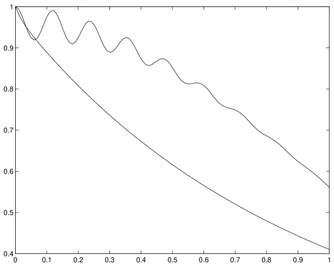
Figure 6: The intensity of the centre line as a function of the transit time in the interval $0<\tau<1$. The upper curve depicts the QM model, and the lower curve the stochastic model. The parameter $\gamma$ has been taken as 0.2.

I have plotted $\rho_{0}^{\text{S}}\left(\tau\right)$ in the range $0<\tau<1,$ including a plot of $\overline{\rho_{0}^{\text{Q}}}\left(\tau\right)$ for comparison.

The new stochastic model indicates the role of the states of odd momentum. They have an intensity of order $\gamma^{2}$, because the transition time from an upper to a lower atomic state is smaller than that of the reverse transition by a factor of order $\gamma^{2}$. This indicates a crucial role for the zeropoint electromagnetic field (ZPEF) which has also played an important role in the program, developed by Emilio Santos and myself[9][10], and designed to achieve a local realist understanding of the optical Bell experiments. When the detuning frequency exceeds the resonant Rabi frequency, ”spontaneous” transitions, that is transitions induced by the ZPEF, are more frequent than laser-induced ones. Note that the new stochastic model differs radically from the QM model for the case that the incoming atom is in its upper state, because in that case the fast transition, with probability proportional to $\gamma^{-2}$, occurs first. This gives a spectrum with strong lines at $n=\pm 1/2,\pm 3/2\ldots,$ and weak lines at $n=0,\pm 1,\pm 2\ldots,$ that is a reversal of the pattern shown for an incoming atom in its lower state. The QM model predicts no difference between these two spectra, so the discrepancy may provide an experimental method for determining which is the more correct out of the two models.

6 Discussion

Before discussing the disagreements between the QM and stochastic models, I emphasize the agreement we obtained in the asymptotic limit $\tau\rightarrow\infty.$ It is easily shown that the choice of $\alpha\left(\zeta\right)$ and $\beta\left(\zeta\right)$ made in (27) is, up to a phase shift in $\zeta$, the only one which gives asymptotic agreement with the QM model. There is a simple explanation for this, namely that, in the stochastic model, the drift in an interval $\tau$ is $\tau\left[\alpha\left(\zeta\right)-\beta\left(\zeta\right)\right]$, which, with the choice we have made, becomes $\tau\sin 2\zeta$. This, without diffusion, is precisely the deterministic model occurring in Section 2 as the classical limit of the QM model (see Fig.2). Hence the deterministic parts of both the QM and stochastic models give the same results.

The disagreement between the models, which we found for very small $\tau$, may well be irrelevant, since the QM model has very rapid oscillations (see Fig.3), and we have just seen that the modified Markov model also produces a radical change in the intensities for very small $\tau$. The quantum mechanical behaviour, whereby the initial probability of transition from a pure state changes from 1 by a quantity proportional to $\tau^{2},$ is a general characteristic, called the Quantum Zeno Paradox, according to which a continuously observed system cannot undergo a transition. This paradox has never received a satisfactory resolution. On the other hand $\left\langle n^{2}\right\rangle$ is proportional initially to $\tau$ for any Markov process. Note, however, that, although Fig.6, like the first diagram in Fig.5, does indeed show an initial decrease in $\rho_{0}^{\text{S}}$ proportional to $\tau$, compared with $\tau^{2}$ for both $\rho_{0}^{\text{Q}0}$ and $\overline{\rho_{0}^{\text{Q}}},$ the initial curvature of the latter is very large compared with that of the former, which means that direct observation of the Zeno phenomenon would be extremely difficult.

I turn finally to the disagreement shown in Fig.5, in particular the oscillatory behaviour of $\rho_{n}^{\text{Q}0}\left(\tau\right)$. We need to know the extent to which this behaviour of the line intensity is actually supported by experiment, in particular whether the observed spectrum is consistent with (36a). If the existence of zero-intensity lines for certain $\tau$ is confirmed by experimental evidence, then the class of stochastic processes may have to be extended to allow for the possibility that the atom has a memory of a recent transition having occurred.

The comparison I have made between the QM and stochastic models, or between the wavelike ”atom” of Fig.1 and the more recognizably atomic object of Fig.4, indicates to me that the atom of Democritus, or of Boltzmann, is by no means dead. Inequality (36a) provides us with a means to determine which of these simple models gives the better agreement with experiment. It would also be interesting to try repeating the experiment with an incoming beam of atoms in the upper state, to see whether the pattern of strong and weak lines is actually inverted, as predicted in the stochastic model.

References

[1] S. G. Brush, The Kind of Motion We Call
Heat, North-Holland, Amsterdam (2 vols.) (1976)
[2] P. L. Gould, Am. J. Phys., 62, 1046-1050
(1994)
[3] P. L. Gould P. J. Martin, B. G. Oldaker, A. H. Miklich and
D. E. Pritchard, Phys. Rev. A, 36, 2495 (1987)
[4] P. L. Gould, P. J. Martin, G. A. Ruff, E. Stoner, J-L. Picqué and D. E. Pritchard Phys. Rev. A, 43, 585
(1991)
[5] P. L. Kapitza and P. A. M. Dirac, Proc. Camb. Phil.
Soc., 29, 293 (1933)
[6] T. G. Kuhn, Black Body Radiation and the Quantum
Discontinuity 1894-1912, Clarendon, Oxford (1978)
[7] M. S. Bartlett, Stochastic Processes
University Press, Cambridge (1960)
[8] I. S. Gradshteyn and I. M. Ryzhik, Table of Integrals,
Series and Products, Academic, New York, formulae 8.453 and 8.454
(1979)
[9] T. W. Marshall and E. Santos, Phys. Rev. A39 6271-6283 (1989)
[10] T. W. Marshall and E. Santos, Recent Res. Devel. Optics2 693-717 (2002).
See also the Internet pages
homepages.tesco.net/~trevor.marshall and
arXiv.org/quantph/abs/0203042