Effective boson-spin model for nuclei ensemble based universal quantum memory

Abstract

We study the collective excitation of a macroscopic ensemble of polarized nuclei fixed in a quantum dot. Under the approximately homogeneous condition that we explicitly present in this paper, this many-particle system behaves as a single mode boson interacting with the spin of a single conduction band electron confined in this quantum dot. Within this effective spin-boson system, the quantum information carried by the electronic spin can be coherently transferred into the collective bosonic mode of excitation in the ensemble of nuclei. In this sense, the collective bosonic excitation can serve as a stable quantum memory to store the quantum spin information of electron.

I Introduction

In the current development of quantum information science and technologies, people have devoted much effort searching for the optimal system serving as a long-lived quantum memory to store the quantum information carried by a quantum system with short decoherence time q-infor . A universal quantum information storage can be understood as a physical process to encode the states of each qubit (rather than the general quantum state) into the states of the quantum memory with much longer decoherence time than the life time of qubit za-store ; or transform the quantum information carried by a quantum system (such as photons) which is difficult to manipulate to an easily controllable system (such as the localized atomic ensemble) sun-prl . Such quantum information storages are absolutely necessary in both measurement based quantum computation schemes Knill ; zhou and two-qubit gate-based computation schemes U-gate .

In the past years the collective excitation of the ensemble of atoms have been proposed to serve as quantum memory for photon information Lukin-RMP . Several experiments lui ; lukin-exp ; kimble have already demonstrated the central principle of this scheme. These schemes work to record the Fock states of photon or their coherent superpositions. In this paper we will pay attention to the universal quantum storage (called qubit storage) that stores the basic two-level state, the state of qubit rather than a general quantum state za-store . The universality of the qubit storage lies on the fact that a general quantum state can be encoded as the state of multi-qubits and the corresponding quantum logic operations can be decomposed into the ”quantum networks” which are the product of the fundamental operations defined with respect to the qubits U-gate .

In usual, the foundation of a universal scheme of quantum information storage depends on whether one can discover a new quantum system with much long decoherence time as the universal quantum memory. Recently a novel protocol for universal quantum information storage was presented based on the nanomechanical resonator interacting with charge qubits. As the universal quantum memory, the nanomechanical resonator behaves as a single mode harmonic oscillator and its coupling to charge qubit is just described by the Jaynes-Cummings (JC) model cleland . Such spin-boson interaction forms the basis for ion-trap based computation schemes as well ion . These idealized schemes motivate us to seek another more practical protocol based on collective bosonic excitation in various physical systems. We notice that a mesoscopic system that consists of finite nuclear spins attached in a quantum dot has been proposed to realize a long-lived quantum memory in this universal way uqm-lukin ; uqm-zoller ; uqm-exp . The present article will start from this basic idea and then work on the macroscopic limit that the number of polarized nuclei is very large so as to be treated approximately as infinite.

We will show that, under two independent sufficiently approximately homogeneous conditions, the collective excitation of a macroscopic ensemble of polarized nuclei fixed in a quantum dot can behave as a single bosonic mode. In this sense, confined in this quantum dot, the spin of a single conduction band electron interacts with this collective excitation and then forms an effective spin-boson system. It demonstrates a dynamic process to coherently store the quantum information carried by the electronic spin in the collective bosonic mode of the nuclei ensemble. Then the collective excitation of the nuclei ensemble can serve as a universal quantum memory to store the quantum information of spin state of electron.

II Boson Realization of Collective Excitation in the Ensemble of Polarized Nuclei

We can consider the ensembles of $N\sim 10^{3-5}$ polarized nuclei with spin $I_{0}$, which are fixed in a charged quantum dot and interact with a single conduction band electron confined in this dot (Fig. 1). There exists a hyperfine contact interaction between the s-state conduction electron and the fixed nuclei. When a static magnetic field is applied to the dot, the effective Hamiltonian for the total system reads

$$H = \Omega_{z}\sigma_{z}+\omega_{z}\sum_{j=1}^{N}I_{z}^{(j)}$$ (1)

$$+\sigma_{z}\sum_{j=1}^{N}g_{j}I_{z}^{(j)}+\sigma_{+}\sum_{j=1}^{N}\frac{g_{j}}{2}I_{-}^{(j)}+h.c,$$

where the operators

$$\mathbf{I}^{(i)}=(I_{x}^{(i)},I_{y}^{(i)},I_{z}^{(i)})$$ (2)

and

$$\mathbf{\sigma}=(\sigma_{x},\sigma_{y},\sigma_{z})$$ (3)

describe the spins of the nucleus at $i$th site and the conduction electron respectively. The coefficients $\Omega_{z}$ and $\omega_{z}$ are the Larmor precession frequencies of nucleus and electron which are linearly determined by the applied external magnetic field. The strength $g_{i}$ of the hyperfine interaction depends on the local value of the norm $\left|\psi(x_{i})\right|^{2}$ at the position $x_{i}$ of $i$th nucleus, while $\psi(x_{i})$ is the wave packet of a single electron inside the dot. In this article, we take the average of couplings as $\overline{g}=\sum_{i}g_{i}/N=A/N$ . Here, we have also used the spin-flip operators

$$\sigma_{\pm}=\left(\sigma_{x}\pm i\sigma_{y}\right)/2$$ (4)

and

$$I_{\pm}^{\left(j\right)}=\left(I_{x}^{\left(j\right)}\pm iI_{y}^{\left(j\right)}\right)/2.$$ (5)

In the following discussion, the eigenstates of $\sigma_{z}$ and $I_{z}^{\left(j\right)}$ are denoted as $\left|\uparrow\right\rangle_{e}$, $\left|\downarrow\right\rangle_{e}$ and $\left|m\right\rangle_{j}$ which satisfy

$$\sigma_{z}\left|\uparrow\right\rangle_{e}=\left|\uparrow\right\rangle_{e},\sigma_{z}\left|\downarrow\right\rangle_{e}=-\left|\downarrow\right\rangle_{e}$$ (6)

and

$$I_{z}^{\left(j\right)}\left|m\right\rangle_{j}=m\left|m\right\rangle_{j},m=I_{0},I_{0}-1,...,-I_{0}.$$ (7)

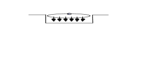
Figure 1: The polarized nuclei interacting with an electron in a quantum dot. Because of the overlap between the electronic wave function and the nuclear wave functions, an effective spin-spin coupling between the electron and the nuclei is induced.

An obvious observation seen from the above expression of the Hamiltonian (1) is that all nuclei wholly couple to a single electron spin. Then we can introduce a pair of collective operators

$$B=\frac{\sum_{i=1}^{N}g_{i}I_{-}^{(i)}}{\sqrt{2I_{0}\sum_{j}g_{j}^{2}}}$$ (8)

and its conjugate $B^{+}$ to depict the collective excitations in the ensemble of nuclei with spin $I_{0}$ from its polarized initial state

$$\left|G\right\rangle=\left|M=-NI_{0}\right\rangle=\prod\limits_{i=1}^{N}\left|-I_{0}\right\rangle_{i},$$ (9)

where $M$ is the eigen value of the $z$-component of total nuclei spin $I_{z}=\sum_{i=1}^{N}I_{z}^{(j)}$, which denotes the saturated ferromagnetic state of nuclei ensemble.

Now we can show that the collective excitations depicted by $B$ and $B^{+}$ can behave as bosons under the ”quasi-homogeneity” conditions in the low excitation limit (we will explicitly present this as follows). In fact, in the previous investigations sun-prl ; sun-pra ; sun-prb , we have proved that, if the coupling is homogeneous or in a periodic way, the collective operators $B$ and $B^{\dagger}$ can indeed be considered as boson operators in the low excitation and macroscopic limit $n/N\rightarrow 0$, where $n$ is the number of excitation from ground state $\left|G\right\rangle$. The number $n$ characterizes the number of collective excitations of the nuclei ensemble, which is defined through the eigenvalue $m_{n}=-NI_{0}+1/2+n$ of the $z$-component of total spin

$$J_{z}=\sigma_{z}+I_{z},$$ (10)

where $n=0,1,2,\cdots,2NI_{0}-1.$ It is obvious that $J_{z}$ is a ”good quantum number” for the Hamiltonian (1) since $\left[J_{z},H\right]=0$. Here, we do not include the saturated ferromagnetic states with $J_{z}=\pm(NI_{0}+1/2)$. It is noticed that $n$ is actually the number of excitations in the system, regardless of mode $B$ or others. There is an intuitive argument that if the $g_{i}$s have different values, but the distribution is ”quasi-homogeneous”, $B$ and $B^{\dagger}$ can also be considered as boson operators satisfying

$$[B,B^{+}]\rightarrow 1$$ (11)

approximately. In the following discussion, we will provide two descriptions  for the ”quasi-homogeneity” condition, under which Eq. (11) holds in the limit $n/N\rightarrow 0$.

To this end we re-write the commutator of $B$ and $B^{\dagger}$ as

$$[B,B^{+}]=-\frac{\sum_{j}g_{j}^{2}I_{z}^{\left(j\right)}}{I_{0}\sum_{j}g_{j}^{2}}\equiv 1-F(N,n),$$ (12)

where

$$F(N,n)=\frac{\sum_{j}g_{j}^{2}\left[I_{z}^{\left(j\right)}+I_{0}\right]}{I_{0}\sum_{j}g_{j}^{2}}.$$ (13)

Since $g_{j}^{2}\leq g_{\max}^{2}$, $F=F(N,n)$ can be estimated as

$$F\leq\frac{g_{\max}^{2}\left(I_{z}+NI_{0}\right)}{\overline{g^{2}}I_{0}N}\leq\frac{g_{\max}^{2}n}{\overline{g^{2}}I_{0}N},$$ (14)

where $\overline{g^{2}}=\sum_{j}g_{j}^{2}/N$ is the average over set $\{g_{j}^{2}\}$. Here we have used the definition of $n$: $I_{z}+I_{0}N=n$ or $n+1$ with respect to the electronic spin up or spin down and the condition $NI_{0}>>1$. Therefore, it is easy to see that when $g_{\max}^{2}/\overline{g^{2}}\sim 1$ in the limit $n/N\rightarrow 0,$ we have $F(N,n)\rightarrow 0$ and then $[B,B^{+}]\simeq 1$. Based on the above argument, the first ”quasi-homogeneity” condition can be obtained as

$$\frac{g_{\max}^{2}}{\overline{g^{2}}}\quad\sim 1.$$ (15)

We would like to point out that the above condition corresponds to the physically relevant case of a quantum dot since $g_{i}$ is proportional to the norm $\left|\psi(x_{i})\right|^{2}$ at the position of nuclei  for the wave packet $\psi(x_{i})$ of a quasi-free electron moving inside the dot.

However, the above ”quasi-homogeneity” condition is not necessary and we can find another independent one as follows. By a straightforward calculation we can also re-express $F(N,n)$ as

$$F=1-\frac{\left(I_{z}+I_{0}N\right)}{I_{0}N}-\frac{\sum_{j}I_{z}^{\left(j\right)}\left[g_{j}^{2}-\overline{g^{2}}\right]}{I_{0}N\overline{g^{2}}}.$$ (16)

Since the term $\left(I_{z}+I_{0}N\right)/\left(I_{0}N\right)\sim n/\left(I_{0}N\right)$ for $N>>1$ and $\left|\left\langle I_{z}^{\left(j\right)}\right\rangle\right|\leq I_{0}$, the upper limit of the second term in the right side of Eq. (16) can be estimated as

$$\left|\frac{\sum_{j}I_{z}^{\left(j\right)}(g_{j}^{2}-\overline{g^{2}})}{I_{0}N\overline{g^{2}}}\right|\leq\left(\overline{\delta g^{2}}\right)/\overline{g^{2}}$$ (17)

in terms of the absolute value deviation

$$\overline{\delta g^{2}}=\frac{1}{N}\sum_{j}\left|g_{j}^{2}-\overline{g^{2}}\right|$$ (18)

of $g_{j}^{2}$. Therefore it is obvious that $[B,B^{+}]\rightarrow 1$ in the low excitation limit $n/N\rightarrow 0$ when another ”quasi-homogeneity” condition

$$\frac{\overline{\delta g^{2}}}{\overline{g^{2}}}\rightarrow 0$$ (19)

holds.

It is pointed out that, both of the two ”quasi-homogeneity” conditions (15) and (19) are sufficient conditions for the boson commutation relation $[B,B^{+}]=1$ , but they are independent with each other and we can obtain neither of them from another. There are some cases in which one of the two conditions is satisfied, but another is violated. For instance, in the case with $N\sim 10^{4}$, if $g_{1}=g_{2}=...=g_{N-1}=g$ and $g_{N}=10g$ then we have $\overline{g^{2}}=1.01g^{2}$, $g_{\max}^{2}=100g^{2}$ and $\overline{\delta g^{2}}\approx 0.02g^{2}$. It is apparent that the condition (15) is violated, but the condition (19) is satisfied since $g_{\max}^{2}/\overline{g^{2}}\approx$ $100$ and $\overline{\delta g^{2}}/\overline{g^{2}}\approx 0.02$. In another example , we take $g_{1}=g_{2}=...=g_{N/2}=g$ and $g_{N/2+1}=g_{N/2+2}=...=g_{N}=3g$, then we have $\overline{g^{2}}=5g^{2}$, $g_{\max}^{2}=9g^{2}$ and $\overline{\delta g^{2}}\approx 4g^{2}$. This is a physically relevant case when the size of electron wave function fixed and the nuclear spin density is increased. It indicates that the condition (19) is violated, but the condition (15) is satisfied in this case.

III Effective Hamiltonian Decorated by External Magnetic Field

As mentioned above the $z$-component of total spin $J_{z}=\sigma_{z}+I_{z}$ is conserved and thus we can classify the total Hilbert space for the ensemble of polarized nuclei according to the excitation number $n.$ In the following we denote the eigenspace of $J_{z}$ with eigenvalue $m_{n}$ by $V_{n}$. Then $V_{n}$ can be decomposed into a direct sum of two eigen-spaces

$$V_{n+}=Span\{\left|g_{k}^{\left(n\right)}\right\rangle|k=1,2..,\}$$ (20)

where the basis vectors

$$\left|g_{k}^{\left(n\right)}\right\rangle\in\{\left|\uparrow\right\rangle\otimes\left|l_{1}l_{2}...l_{N}\right\rangle|\sum_{j}l_{j}=-NI_{0}+n\}$$ (21)

and

$$V_{n-}=Span\{\left|f_{k}^{\left(n\right)}\right\rangle|k=1,2..,\}$$ (22)

where the basis vectors

$$\left|f_{k}^{\left(n\right)}\right\rangle\in\{\left|\downarrow\right\rangle\otimes\left|l_{1}l_{2}...l_{N}\right\rangle|\sum_{j}l_{j}=-NI_{0}+n+1\}$$ (23)

of $I_{z}$, i.e., $V_{n}=V_{n+}\oplus V_{n-}$. Then the Hamiltonian (1) can be decomposed into three parts in the invariant subspace $V_{n},$ namely,

$$H=H_{R}+H_{S}+H_{p}.$$ (24)

Each part $H_{R},H_{S}$ and $H_{p}$ can be described as follows: The first part

$$H_{R}=\Omega\left(\sigma_{+}B+\sigma_{-}B^{+}\right)$$ (25)

is a resonate JC Hamiltonian with the collective Rabi frequency

$$\Omega=\sqrt{I_{0}\sum_{j}\frac{g_{j}^{2}}{2}}$$ (26)

coupling the electron spin to the collective excitation. Associated with the non-collective excited states $\left|g_{k}^{\left(n\right)}\right\rangle$, $\left|f_{k}^{\left(n\right)}\right\rangle$ and the corresponding composite energies

$$\mu_{g}(n) = \frac{\Omega_{z}}{2}+\omega_{z}(m_{n}-\frac{1}{2})-\frac{N\overline{g}I_{0}}{2},$$

$$\mu_{f}(n) = -\frac{\Omega_{z}}{2}+\omega_{z}(m_{n}+\frac{1}{2})+\frac{N\overline{g}I_{0}}{2},$$ (27)

the second part

$$H_{S} = \Omega_{z}\sigma_{z}+\omega_{z}\sum_{j=1}^{N}I_{z}^{(j)}-\sigma_{z}\sum_{j=1}^{N}g_{j}I_{0}$$

$$= \mu_{g}\left(n\right)\sum_{k}\left|g_{k}^{\left(n\right)}\right\rangle\left\langle g_{k}^{\left(n\right)}\right|+\mu_{f}\left(n\right)\sum_{k}\left|f_{k}^{\left(n\right)}\right\rangle\left\langle f_{k}^{\left(n\right)}\right|$$

is derived from the first and second terms of the original Hamiltonian and also operates within the subspace $V_{n}.$ In the third part

$$H_{p} = \sigma_{z}\sum_{j=1}^{N}g_{j}(I_{z}^{(j)}+I_{0})$$

$$= \sum_{k}\sum_{j=1}^{N}\frac{g_{j}}{2}\left(M_{kn}^{\left(j\right)}+I_{0}\right)\left|g_{k}^{\left(n\right)}\right\rangle\left\langle g_{k}^{\left(n\right)}\right|$$

$$-\sum_{k}\sum_{j=1}^{N}\frac{g_{j}}{2}\left(M_{kn}^{\prime\left(j\right)}+I_{0}\right)\left|f_{k}^{\left(n\right)}\right\rangle\left\langle f_{k}^{\left(n\right)}\right|$$

$M_{kn}^{\left(j\right)}$ ($M_{kn}^{\prime\left(j\right)}$) is the $c$-number which describes the $z$ component of the $j$-th nuclear spin in the state $\left|g_{k}^{\left(n\right)}\right\rangle$ ( $\left|f_{k}^{\left(n\right)}\right\rangle$).

We observe that the interaction part $H_{JC}=H_{R}+H_{S}$ is very similar to the Jaynes-Cummings (JC) Hamiltonian in cavity QED describing the interaction between the two-level atom and single-mode electromagnetic field in the rotating wave approximation. In order to create the entanglement between electron spin and collective bosons, one can adjust the external field $B_{0}$ so that $\mu_{f}(n)=\mu_{g}(n)$, that is

$$\Omega_{z}=\omega_{z}+N\overline{g}I_{0}$$ (30)

In this case $H_{JC}$ $=\oplus_{n}H_{JC}^{[n]\text{ }}$on the whole space $V=\oplus_{n}$ $V_{n}$ can be reduced to the irreducible parts

$$H_{JC}^{[n]}\sim H_{R}+n\omega_{z}$$ (31)

for $\omega_{z}=\Omega_{z}-N\overline{g}I_{0}$. Correspondingly the dynamics of the total system can also be constrained within the invariant subspace $V_{n}$ and then the last term $n\omega_{z}$ independent of $\sigma_{+}$and $B$ can be ignored since it can not contribute to the dynamics of the system significantly.

To consider the effectiveness of the above qubit storage protocol, we need to analyze the role of other collective modes orthogonal to the basic collective model defined by $B$ and $B^{+}$. These auxiliary collective modes complement the ”$B$” mode to generate a complete Hilbert space of the nuclei ensemble.In fact, we can generally construct the complete set of creation and annihilation operators $C_{k}^{+}$ and $C_{k}$ ( $k=1,2,...,N$ ) including $C_{0}=B$ and all auxiliary modes as

$$C_{k}=\frac{\sum_{i=1}^{N}h_{i}^{[k]}I_{+}^{(i)}}{\sqrt{2I_{0}\sum_{j}h_{j}^{2}}}.$$ (32)

where

$$\mathbf{h}^{[k]}=(h_{1}^{[k]},h_{2}^{[k]},...,h_{N}^{[k]})$$ (33)

(for $k=1,2,...,N$) are $N$ orthogonal vectors in the $N$-dimension space $\mathbf{R}^{N}$, which can be systematically constructed by making use of the Gramm-Schmidt orthogonalization method starting from

$$\mathbf{h}^{[1]}=(g_{1},g_{2,}...,g_{N})\in\mathbf{R}^{N}.$$ (34)

Since $\mathbf{h}^{[k]}\cdot\mathbf{h}^{[j]}=\delta_{kj}$ and the Gramm-Schmidt orthogonalization can also result in the quasi-homogeneity conditions

$$\frac{\overline{\delta h^{{}^{[k]}2}}}{\overline{h^{{}^{[k]}2}}}\sim 0,or\qquad\frac{h_{\max}^{{}^{[k]}2}}{\overline{h^{{}^{[k]}2}}}\sim 1\qquad$$ (35)

we have

$$[C_{k},C_{j}^{+}]\rightarrow\delta_{kj}$$ (36)

in the large $N$ limit.

For example, one can construct a new boson mode with respect to the existing mode by the collective excitation $B$ by choosing a new distribution of coupling constants

$$\{h_{i}|h_{i}=g_{N-i,\text{ }}h_{N-i}=-g_{i},\forall i<\frac{N}{2}\}$$ (37)

as a permutation of $\{g_{i}\}$ and then define a independent boson mode by the collective operator $C$ as Eq. (32). We can check that both the orthogonal relation $\sum_{i=1}^{N}g_{i}h_{i}=0$ and the quasi-homogeneity conditions $\overline{\delta h^{2}}/\overline{h^{2}}\sim 0$ or $h_{\max}^{2}/\overline{h^{2}}\sim 1$ can be satisfied obviously. Then one can prove that in each invariant subspace $V_{n}$ with $n\ll N$ , there are the typical boson commutation relations

$$[C,C^{+}]=1,[C,B^{+}]=0.$$ (38)

Apparently, from the above generalized the Gramm-Schmidt orthogonalization, the auxiliary boson operators can be expressed as the linear combination of the spin operators through a matrix transformation $\mathbf{C}=U\mathbf{I}$ for

$$\mathbf{C} = \left(B,C_{2},...,C_{N}\right)^{T},$$ (39)

$$\mathbf{I} = \left(I_{-}^{\left(1\right)},I_{-}^{\left(2\right)},...,I_{-}^{\left(N\right)}\right)^{T},$$

where $U$ is a unitary (or orthogonal) matrix. Since $\mathbf{C}^{+}\mathbf{C=I}^{+}\mathbf{I=}\sum_{j=1}^{N}I_{+}^{\left(j\right)}\mathbf{\ }I_{-}^{\left(j\right)}$ under such transformation one can prove that there exists a constraint

$$B^{+}B+\sum_{k}C_{k}^{+}C_{k}\approx I_{z}+I_{0}N.$$ (40)

when they work on the subspace $V_{n}$ with $n\ll N.$

$$\Omega_{z}=\omega_{z}+N\overline{g}I_{0}.$$ (41)

Formally, the Hamiltonian in Eq. (31) can be rewritten in the whole space as

$$H_{JC} = H_{R}+\omega_{z}I_{z}+\Omega_{z}\sigma_{z}-\sigma_{z}\sum_{j=1}^{N}g_{j}I_{0}$$ (42)

$$\sim H_{R}+\omega_{z}\sum_{k}C_{k}^{+}C_{k}+\omega_{z}(B^{+}B+\sigma_{z})$$

according to the above constraint. The above argument implies no coupling between the basic mode $B$ and the auxiliary modes $C_{k}$ $($ $k=1,2,...,N-1)$ and thus the dependence on $C_{k}$ is trivial in the above equation. However, all mode coupling terms between the auxiliary modes $C_{k}$ and the electron spin qubit occur only in $H_{p}$, which can cause decoherence of the qubitloss . In section VI we will explore this decoherence mechanism in details.

IV Validity of the Single Mode Approximation

First, let’s assume that $B$ mode is independent of those auxiliary collective modes $C_{k}$. To formally diagonalize $H_{JC}$ by straightforward calculations, one can obtain the eigenvalues of $H_{JC}$

$$E_{\pm}({m_{i}},m)=(m+\sum_{i}m_{i})\omega_{z}\pm\sqrt{I_{0}\left(m+1\right)\sum_{j}\frac{g_{j}^{2}}{2}}$$ (43)

and the corresponding eigenstates:

$$\left|\psi^{(\pm)}\left(\left\{m_{i}\right\},m\right)\right\rangle = \frac{1}{\sqrt{2m!m_{i}!}}\left(\left|\uparrow\right\rangle_{e}\pm\left|\downarrow\right\rangle_{e}\frac{B^{+}}{\sqrt{m+1}}\right)$$ (44)

$$\otimes(B^{+})^{m}(C_{i}^{+})^{m_{i}}\left|G\right\rangle$$

where we have $\sum_{i}m_{i}+m=n$.

It is also pointed out that, only the ”excited” nuclear spins whose $z$ component values are not $-I_{0}$ have contributions to the summation in the definition of $H_{p}$ (III). Therefore, because of the low exciton condition, there is an intuitive argument to show that $H_{p}$ is only a perturbation term. In the following, this guess can be proved explicitly. Under the quasi-homogeneity conditions (15) and (19), one has

$$H_{p}\sim\frac{\bar{g}}{2}\left(I_{z}+NI_{0}\right)\sigma_{z},$$ (45)

where $\bar{g}=A/N$ is the average coupling strength between the electron and nuclei. Then the first order energy correction for $H_{p}$ can be estimated with perturbation theory:

$$\delta E\left(n\right)\sim\left\langle\psi_{n}^{(\pm)}\right|H_{p}\left|\psi_{n}^{(\pm)}\right\rangle\sim\frac{n}{4}\bar{g}.$$ (46)

On the other hand, the energy gap between $E_{\pm}(n)$ is

$$\Delta E(\left\{m_{i}\right\},m) = \sqrt{I_{0}(m+1)\sum_{j}\frac{g_{j}^{2}}{2}}$$ (47)

$$\sim \frac{\overline{g}}{\sqrt{2}}\sqrt{NI_{0}\left(m+1\right)}$$

where we have used the relation $\overline{g^{2}}\sim\bar{g}^{2}$, which meets the conditions (15) and (19). Therefore, the magnitude of the contribution of $H_{p}$ can be described by the ratio

$$\left|\frac{\delta E\left(n\right)}{\Delta E(\left\{m_{i}\right\},m)}\right|\sim\sqrt{\frac{n}{N}}.$$ (48)

The above estimation implies that $H_{p}$ can indeed be regarded as perturbation to $H_{JC}$ in the low excitation case and macroscopic limit $n\ll N$. Therefore, we can take $H_{JC}$ as the effective Hamiltonian of the total system. It is noticed that, there is no coupling between the mode $B$ and the auxiliary modes $C_{k}$. Hence we can write down the effective Hamiltonian of the electron spin and the $B$ mode as

$$H_{c}=\Omega(\sigma_{+}B+\sigma_{-}B^{+})+\omega_{z}\left[B^{+}B+\sigma_{z}-1/2\right].$$ (49)

In order to quantitatively evaluate the extent of approximation of the single mode boson approach and obtain the effective Hamiltonian, the numerical method is employed to verify our approximate analytical result. We compute the eigenstates of the original spin-exchange Hamiltonian

$$H_{s}=\frac{1}{2}\sum_{j}g_{j}(\sigma_{+}I_{-}^{(j)}+\sigma_{-}I_{+}^{(j)})$$ (50)

and

$$H_{c}-n\omega_{z}=\Omega(\sigma_{+}B+\sigma_{-}B^{+}).$$ (51)

for finite $N$ system. Without loss of generality we take a Gaussian type distribution which satisfies the conditions (15) and (19). In Fig.2, the spectrums of $H_{s}$ and $H_{c}-n\omega_{z}$ for $N=80$ and $I_{0}=1/2$ system in the subspace $J_{z}=-N/2+1$ are plotted in (a) and (b). It shows that the spectrums are in agreement with each other. By comparing the numerically exact results with the analytically approximate ones for the effective spin-boson system, the numerical result shows that in low excitation and macroscopic limit with the quasi-homogeneity condition, the single mode boson effective Hamiltonian (49) can work well in describing the collective excitation of the nuclei ensemble stimulated by the conduction band electron. We can also understand the difference of the spectrum structures in Fig. 2 in terms of the concept of ”hardcore boson” fisher . We imagine a model Hamiltonian $H_{b}=H_{s}(I_{-}^{(j)}\rightarrow b^{(j)})$, which is obtained by replacing $I_{-}^{(j)}$ ($I_{+}^{(j)}$) in Eq. (50) with a set operators $b^{(j)}(b^{(j)+})$. If they satisfy the usual commutation relation of bosons that the operators $b^{(j)+}(b^{(j)})$ and $b^{(k)}(b^{(k)+})$ on different sites commute with each other, then $B$ and $B^{+}$ automatically satisfy the boson commutation relation and then result in the regular spectrum same as to that illustrated in Fig. 2(b). However, if the bosons are of hardcore, i.e., they are repulsive with each other at a same site, one can describe them with vanishing anti-commutators $\{b^{(j)+},b^{(j)+}\}=0$ for the same site and the vanishing commutators $[b^{(j)\pm},b^{(k)\pm}]=0$ for different sites. In this case the repulsive interaction with hardcore feature will widen the original spectral lines to form the similar band structure in the energy spectrum.

Figure 2: The spectrums of $H_{s}$ (a) and $H_{c}-\omega_{z}$ (b) for $N=80$ and $I_{0}=1/2$ system in the subspace $J_{z}=-N/2+1$. The slight deviation between the two spectrums is due to the hardcore effect of two bosons and should vanish in macroscopic limit.

V Quantum Information Storage as a Dynamical Process

We notice that the above effective Hamiltonian is just of the JC type on the resonance and then it can be used to produce the entanglement between the qubit state of the electron and the bosonic mode of the collective excitation of the nuclei ensemble. Thus this entanglement induces a writing process of qubit information into the collective excitation.

We assume that the initial state of the total system

$$\left|\psi(0)\right\rangle=\left|d(0)\right\rangle_{e}\otimes\left|G\right\rangle$$ (52)

contains the arbitrary superposition

$$\left|d(0)\right\rangle_{e}=\alpha\left|\uparrow\right\rangle_{e}+\beta\left|\downarrow\right\rangle_{e}$$ (53)

of electronic states and define the Fock state

$$\left|m\right\rangle_{b}=\frac{1}{\sqrt{m!}}(B^{+})^{m}\left|G\right\rangle$$ (54)

for the collective excitation. We now consider the long time evolution by projecting the wave function onto each invariant subspace spanned by the states $\left\{\left|\uparrow\right\rangle_{e}\left|m\right\rangle_{b},\left|\downarrow\right\rangle_{e}\left|m+1\right\rangle_{b}\right\}$ (we denote this subspace by $Z_{m}$). Then this evolution of mode $B$ and the electron spin can be explicitly characterized by reduced evolution matrices

$$U_{m}(t)=e^{-i\omega_{z}mt}\left[\begin{array}[]{cc}\cos\Omega_{m}t&-i\sin\Omega_{m}t\\ -i\sin\Omega_{m}t&\cos\Omega_{m}t\end{array}\right]$$ (55)

for $m=0,1,2,...$. Here the dressed Rabit frequency

$$\Omega_{m}=\sqrt{(m+1)}\Omega$$ (56)

depends on the number of collective excitation. A storage process of qubit information is expressed by the factorization map

$$\left|d(0)\right\rangle_{e}\otimes\left|G\right\rangle \longrightarrow \left|\downarrow\right\rangle_{e}(\beta\left|G_{1}\right\rangle-i\alpha e^{-i\omega_{z}\pi/2\Omega}\left|G_{2}\right\rangle)$$ (57)

$$= \left|\downarrow\right\rangle_{e}W(\alpha\left|G_{1}\right\rangle+\beta\left|G_{2}\right\rangle)$$

at $t=\pi/2\Omega$. Here $\left|G_{1}\right\rangle=\left|G\right\rangle,\left|G_{2}\right\rangle=(B^{+})\left|G\right\rangle$ are two collective excitation states which are orthogonal with each other, and

$$W=\left[\begin{array}[]{cc}0&1\\ -ie^{-i\omega_{z}\pi/2\Omega}&0\end{array}\right]$$ (58)

is a unitary transformation.

The same case was also encountered in Ref. [10] (see the difference between the initial and final states in Eq. (2) of Ref. [10]). In quantum information theory this can be easily implemented by a local unitary transformation independent of the initial state $\left|d(0)\right\rangle_{e}$ (or the coefficients $\alpha$ and $\beta)$ So the decoding process can easily map back from the final state of the quantum memory

$$\left|F\right\rangle=\beta\left|G_{1}\right\rangle-i\alpha e^{-i\omega_{z}\pi/2\Omega}\left|G_{2}\right\rangle$$ (59)

by its inverse transformation $W^{-1}$. In this sense, we say that the above map implements the quantum information storage. We notice that this is very similar to the case in quantum teleportation, in which the initial state-independent transformation can easily be implemented by Bob for the teleported state once the 2-bit classical information is told by Alice.

However, if one prepares the quantum memory not in its perfectly polarized state $\left|G\right\rangle$ (e.g. $\left|m\right\rangle_{b}$ ($m\neq 0$)), the general initial state

$$\left|\psi(0)\right\rangle=(\alpha\left|\uparrow\right\rangle_{e}+\beta\left|\downarrow\right\rangle_{e})\otimes\left|m\right\rangle_{b}$$ (60)

will evolve into

$$\left|\psi(t)\right\rangle = \alpha U_{m}(t)\left|\uparrow\right\rangle_{e}\left|m\right\rangle_{b}+\beta U_{m-1}(t)\left|\downarrow\right\rangle_{e}\left|m\right\rangle_{b}$$ (61)

$$= \alpha e^{-im\omega_{z}t}\cos\left(\Omega_{m}t\right)\left|\uparrow\right\rangle_{e}\left|m\right\rangle_{b}$$

$$+\beta e^{-i(m-1)\omega_{z}t}\cos\left(\Omega_{m-1}t\right)\left|\downarrow\right\rangle_{e}\left|m\right\rangle_{b}$$

$$-i\beta e^{-i(m-1)\omega_{z}t}\sin\left(\Omega_{m-1}t\right)\left|\uparrow\right\rangle_{e}\left|m-1\right\rangle_{b}$$

$$-i\alpha e^{-im\omega_{z}t}\sin\left(\Omega_{m}t\right)\left|\downarrow\right\rangle_{e}\left|m+1\right\rangle_{b}.$$

It is noticed that in order to obtain the above result, we have considered $\left|\uparrow\right\rangle_{e}\otimes\left|m\right\rangle_{b}$ and $\left|\downarrow\right\rangle_{e}\otimes\left|m\right\rangle_{b}$ which belong to different subspaces $Z_{m}$ and $Z_{m-1}$. Hence they are driven by two different blocks $U_{m}(t)$ and $U_{m-1}(t)$ of the block-diagonal evolution matrix $U=diag[U_{m}(t)]$, respectively. The above result from a straightforward calculation shows that only the ensemble of nuclei, which is prepared in the collective ground state, the polarized ensemble, can serve as a quantum memory. Otherwise there must exist the systematic error for quantum information processing.

VI Decoherence due to the Couplings with Auxiliary Modes

Finally we need to revisit the quantum decoherence in the process of quantum information storage based on the collective excitation of the polarized nuclei ensemble. The main source of decoherence is due to the existence of the single particle motion described by the perturbation Hamiltonian $H_{p}$. The similar situation was ever considered for the collective excitation in the ensemble of free atoms by one of the present authors (CPS) and his collaborators sun-you . The condition under which we can ignore the perturbation result from non-collective excitations is just of preserving quantum coherence. By making use of the boson modes $C_{k}$, we can expect that the part $H_{p}$ contains the coupling between the spin qubit and $N-1$ auxiliary $C_{k}$-modes. This will realize a typical quantum decoherence model for a two level system coupled to a bath of many harmonic oscillators.

In order to analyze this problem more quantitatively, we describe the single particle motion from the perturbation Hamiltonian $H_{p}$ in terms of the excitation of auxiliary modes. We consider a quasi-homogeneous case $g_{j}\approx g$ , in which

$$H_{p}\approx\sum_{k}(\omega_{z}+\frac{1}{2}g\sigma_{z}C_{k}^{+}C_{k})$$ (62)

where we ignore the coupling term $gB^{+}B\sigma_{z}/2\$since it can only lead a phase shift in the spin qubit. We consider the nuclear ensemble prepared in a thermal equilibrium state

$$\rho_{R}=\frac{1}{Z}\prod_{k}\sum_{n_{k}}\exp(-\frac{\omega_{z}n_{k}}{k_{B}T})|n_{k}\rangle\langle n_{k}|$$

where

$$Z=\prod_{k}\sum_{n_{k}}\exp(-\frac{\omega_{z}n_{k}}{k_{B}T})$$ (63)

the partition function at the temperature $T$ where $k_{B}$ is the Boltzman constant. Let the spin qubit be initially in a pure state $\left|\phi\right\rangle=\alpha\left|0\right\rangle+\beta\left|1\right\rangle$. After a straightforward calculation we obtain the density matrix at time $t$

$$\rho\left(t\right)=U\left(t\right)(\left|\phi\right\rangle\left\langle\phi\right|\otimes\rho_{R})U^{-1}\left(t\right)$$ (64)

and the corresponding reduced density matrix $\rho_{S}\left(t\right)=Tr_{B}\rho\left(t\right)$ by tracing over the auxiliary modes $\{C_{k}\}$. The off-diagonal elements of $\rho_{S}\left(t\right)$ can be given explicitly as

$$\rho_{S}^{\star}\left(t\right)_{10} = \rho_{S}\left(t\right)_{01}$$

$$= \frac{\alpha^{\star}\beta(e^{\frac{\omega_{z}}{k_{B}T}}-1)^{N-1}e^{i\left(N-1\right)\theta}}{\sqrt{(e^{\frac{2\omega_{z}}{k_{B}T}}-2e^{\frac{\omega_{z}}{k_{B}T}}\cos(gt)+1)^{N-1}}}$$

where

$$\theta=\arctan\frac{\sin\left(gt\right)}{\exp\left(\frac{\omega_{z}}{k_{B}T}\right)-\cos\left(gt\right)}$$ (66)

In the zero temperature limit or $T\rightarrow 0$, there is no decoherence since the off-diagonal elements

$$\rho_{S}^{\star}\left(t\right)_{10}=\rho_{S}\left(t\right)_{01}=\alpha^{\star}\beta$$ (67)

do not change. But in a finite temperature, the norm of off-diagonal element is proportional to the so-called decoherence factor

$$D(T,t) = d(T,t)^{N-1}$$ (68)

$$\equiv \frac{(e^{\frac{\omega_{z}}{k_{B}T}}-1)^{N-1}}{\sqrt{(e^{\frac{2\omega_{z}}{k_{B}T}}-2e^{\frac{\omega_{z}}{k_{B}T}}\cos(gt)+1)^{N-1}}}.$$

This result illustrates that thermal excitation of the auxiliary modes will block the implementation of the macroscopic nuclear ensemble based quantum memory since in the large $N$ limit $D(T,t)\rightarrow 0$ except for the special instances at

$$t=\frac{2k\pi}{g},k=0,1,2...$$ (69)

In these instances, $D(T,t)=1$ and there is no decoherence at all. Besides, since in these instances $\rho_{S}^{\star}\left(t\right)_{10}=\alpha^{\star}\beta$ is just the initial values and then we implement a ideal quantum information storage to recover the stored state. To further consider the temperature dependecne of the auxiliary mode induced decoherence, we plot a $3D$-graphic of $D(T,t)$ for a small size $N=20$ system. It shows that the case $D(T,t)=1$ appears periodically as time $t$, and $D(T,t)\rightarrow 1$ all the time when $T\rightarrow 0$. According to the experimental data uqm-zoller , the period is roughly estimated as $2\pi/g\sim 10^{-7}s$.

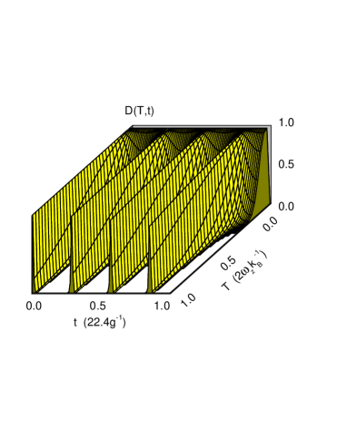
Figure 3: The decoherence factor $D(T,t)$ for a small size system as the function of time and temperature.

VII Summary with Remarks

In summary we have studied the possibility of quantum memory by using collective excitation of ensemble of polarized nuclei surrounding a single electronic spin in a quantum dot. We explicitly present the quasi-homogeneous independent conditions, under which the many-particle system, a macroscopic ensemble of polarized nuclei, can be treated as a single mode bosonic system. Thus the interaction is of the similar form of Jaynes-Cummings model. Based on this fact, the collective excitation can serve as a quantum memory to store the spin state of a conduction electron.

We also pointed out that the physical system for quantum information storage is the same as that in Ref. [10] which first showed that electronic spin coherence can be reversibly mapped onto the collective state of the surrounding nuclei. But our studies emphasize that the collective excitation-based quantum memory can be understood in terms of the spin-boson model with essential simplicity in physics. Especially the valid conditions are discovered in present paper. That is, the collective operators are explicitly invoked to depict the bosonic collective excitations and then we can present an effective boson-spin model, which reveals physical mechanism with collective quantum coherence behind the original conceptual protocol for the long-lived quantum memory.

There are two sources of quantum decoherence in such quantum information processing, one is due to non-collective mode and the other is due to the nuclear spin diffusion or coupling with environment. The latter is dominate and has been well considered in Ref. Phi , but the former can still play a role in certain cases. So we stress the former in this paper since the same situation was even considered for the collective excitation in the ensemble of free atoms by us sun-you . In principle, the latter can also be treated in our spin-boson model with similar approach by adding diffusion terms. We also noticed that the systematic errors in transferring quantum information can occur due to the appearance of higher excitation by illustrating that only the ensemble of nuclei prepared in the collective ground state rather than the excited ones can serve as a quantum memory. How to avoid the higher excitation of the collective boson mode and how to correct the error due to the appearance of higher excitation are open questions that need further investigations.

We acknowledge the support of the CNSF (grant No. 90203018, 10474104), the Knowledge Innovation Program (KIP) of the Chinese Academy of Sciences, the National Fundamental Research Program of China (No. 001GB309310) and Science and Technology Cooperation Fund of Nankai and Tianjin University.

References

- (1) Electronic address: songtc@nankai.edu.cn
- (2) Electronic address: suncp@itp.ac.cn
- (3) Internet www site: http://www.itp.ac.cn/~suncp
- (4) D. Bouwmeeste, A. Ekert, and A. Zeilinger (Ed.), The Physics of Quantum Information (Springer, Berlin, 2000); D. P. DiVincenzo and C. Bennet, Nature 404, 247 (2000) and references therein.
- (5) E. Pazy, I. D’Amico, P. Zanardi, and F. Rossi, Phys. Rev. B 64, 195320 (2001).
- (6) C. P. Sun, Y. Li, and X. F. Liu, Phys. Rev. Lett. 91, 147903 (2003).
- (7) Knill et al., Nature 409, 46 (2001).
- (8) D. L. Zhou, B. Zeng, Z. Xu, and C. P. Sun Phys. Rev. A 68, 062303 (2003).
- (9) A. Barenco et al Phys. Rev. A 52, 3457 (1995).
- (10) M. D. Lukin, Rev. Mod. Phys. 75, 457 (2003).
- (11) C. Liu, Z. Dutton, C. H. Behroozi, and L. V. Hau, Nature 409, 490 (2001).
- (12) C. H. van der Wal, M. D. Eisaman, A. Andre, R. L. Walsworth, D. F. Phillips, A. S. Zibrov, M. D. Lukin, Science 301, 196 (2003).
- (13) A. Kuzmich, W. P. Bowen, A. D. Boozer, A. Boca, C. W. Chou, L.-M. Duan and H. J. Kimble, Nature, 423, 734, (2003).
- (14) A. N. Cleland and M. R. Geller Phys. Rev. Lett. 93, 070501 (2004) .
- (15) D. Leibfried, R. Blatt, C. Monroe, and D. Wineland, Rev. Mod. Phys. 75, 281-324 (2003).
- (16) J. M. Taylor, C. M. Marcus, and M. D. Lukin Phys. Rev. Lett. 90, 206803 (2003).
- (17) A. Imamolu et al., Phys. Rev. Lett. 91, 017402 (2003).
- (18) M. Poggio et al., Phys. Rev. Lett. 91, 207602 (2003).
- (19) Y. X. Liu , C.P. Sun, S. X.Yu, et al., Phys. Rev. A 63, 3802 (2001).
- (20) G. R. Jin, P. Zhang, Y.X. Liu, and C. P. Sun, Phys. Rev. B 68, 134301 (2003).
- (21) A. J. Leggett, S. Chakravarty, A. T. Dorsey, M. P. A. Fisher, A. Garg, and W. Zwerger Rev. Mod. Phys. 59, 1-85 (1987);Divincenzo and Loss, cond-mat/0405525.
- (22) M.P.A. Fisher, P.B. Weichman, G. Grinstein, and D.S. Fisher, Phys. Rev. B 40, 546(1989).
- (23) D. F. Phillips, A. S. Zibrov, M. D. Lukin, Science, 301, 196 (2003).
- (24) C.P. Sun, S.Yi , L.You, Phys. Rev. A 67, 063815 (2003).