Dynamical creation of entanglement by homodyne-mediated feedback

Abstract

For two two-level atoms coupled to a single-mode cavity field that is driven and heavily damped, the steady-state can be entangled by shining an un-modulated driving laser on the system [S.Schneider, G. J. Milburn Phys. Rev A 65, 042107, 2002]. We present a scheme to significantly increase the steady-state entanglement by using homodyne-mediated feedback, in which the driving laser is modulated by the homodyne photocurrent derived from the cavity output. Such feedback can increase the nonlinear response to both the decoherence process of the two-qubit system and the coherent evolution of individual qubits. We present the properties of the entangled states using the SO(3) $Q$ function.

I Introduction

The deeper ways that quantum information differs from classical information involve the properties, implications, and use of quantum entanglement. Entangled states are interesting because they exhibit correlations that have no classical analog. Any two systems described by a pure state that cannot be expressed as a direct product $|{\Psi}\rangle=|{A}\rangle{\otimes}|{B}\rangle$ are entangled (non-separable). For a two-qubit system there are four mutually orthogonal Bell states, which may be denoted

$$|{\phi^{\pm}}\rangle_{AB} = \frac{1}{\sqrt{2}}\left({|{00}\rangle_{AB}\pm|{11}\rangle_{AB}}\right),$$

$$|{\psi^{\pm}}\rangle_{AB} = \frac{1}{\sqrt{2}}\left({|{01}\rangle_{AB}\pm|{10}\rangle_{AB}}\right)$$ (1)

where $A$ and $B$ are two subsystems, $|{0}\rangle$ and $|{1}\rangle$ are two orthogonal states that could represent the atomic ground and excited state, respectively.

Quantum entanglement is a subject of intensive study because it is useful and frequently essential for quantum teleportation Bennett ; Vitali ; Werner , quantum cryptography shor ; Buttler , quantum dense coding Werner and quantum computation Lo ; munro . Also, entangled atoms can be used to improve frequency standards  Dowling1 . Thus, one of the increasing interests in this context is to find ways to generate the right type of entanglement as well as possible Vedral . There are a number of measures, like the concurrence Wootters , entanglement of formation Wootters , entanglement of distillation Rains ; Vedral , relative entropy of entanglement Neumann , and negativity Eisert ; zyczkowski , that have been proposed in recent years for the purpose of quantifying the amount of entanglement.

In this paper we address the question: what is the maximum amount of steady-state entanglement that can be generated in a system consisting of two two-level atoms (qubits) collectively damped, with the output being measured and fed-back to control the system state? This question follows naturally from the study of Schneider and Milburn thesis1 which considered the same system but without measurement or feedback. In both cases the entangled steady state is a mixed state while most quantum entanglement algorithms are designed for ideal pure states. However, it is usually very hard to create, maintain, and manipulate pure entangled states under realistic conditions, simply because any system is subject to the interactions with its external environment. These effects, having their origin in decoherence, may turn pure state entanglement into mixed state entanglement. Therefore it immediately raises the question of whether the entanglement can be distilled and used as a resource for some quantum communication or computation task.

The paper is organized as follows. The model and the corresponding master equation together with the derivation of the adiabatic elimination of the cavity mode for a two-qubit system are analyzed and the steady-state solution is presented in Section II. The entanglement measures and the relationship between purity and entanglement are analyzed in Section III. In section IV, we investigate the behaviour of the $Q$ distribution function and the density matrix in order to obtain information about the entangled states. We discuss our results in the concluding section V.

II Model and master equation

A quantum computer requires that a set of $N$ two-state systems can be prepared in an arbitrary superposition state. Each of these systems is said to encode a qubit, as distinct from the single bit encoded in a classical two state system.

We consider the case where two qubits are coupled to a single cavity mode that is driven and heavily damped. The two qubits undergo spontaneous emission into the cavity mode, and the fluorescence from the output of the cavity is subjected to a homodyne measurement with a subsequent feedback to the cavity. Our primary goal of feedback control in this paper is to demonstrate the ability of feedback control to increase steady-state entanglement by counteracting the effects of both spontaneous emission and the measurement back-action on the system. The history of feedback control in open quantum systems goes back to the 1980s with the work of Yamamoto and co-workers Yamamoto , and Shapiro and co-workersShapiro . Their objective was to explain the observation of fluctuations in a closed-loop photocurrent. They did this using quantum Langevin equations (stochastic Heisenberg equations for the system operators) and also semiclassical techniques. The latter approach was made fully quantum-mechanical by Plimak. For systems with linear dynamics, all of these approaches, and the quantum trajectory approach of Refs.Car93b ; WisMil93a , are equally easy to use to find analytical solutions. The advantage of Wiseman and Milburn’s (quantum trajectory) approach to quantum control via feedback is for systems with nonlinear dynamics, as we will discuss in this paper.

To obtain a master equation for the two-qubit system, we follow the analysis of Schneider and Milburn’s paper thesis1 for the steady-state of a system Cakir of two qubits interacting simultaneously with a driving laser. They have shown that the steady state is entangled. In this work, we expand their analysis to include feedback modulation of the amplitude of the driving laser.

A schematic diagram of the apparatus is shown in Fig.1. To ensure that the two atoms see the same phase and amplitude of the cavity mode, we need to locate them at points of the standing wave in which the two atoms are separated by an integer number of wavelengths. The dipole-dipole interaction between the atoms can thus be ignored in the following calculation. We assume a strong coupling $g$ between the atoms and the cavity mode. The fact that the coupling is the same for both atoms means that they are indistinguishable. This leads to interference in their damping via the cavity, as we shall see. Such a proposed approach can be realized experimentally in a cavity QED system. In this paper we reproduce the results in thesis1 and show that one can increase the steady-state entanglement by using feedback-modulation of the laser that drives the cavity mode.

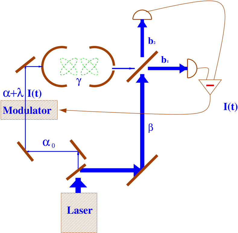
Figure 1: Diagram of the experimental apparatus. The laser beam is split to produce both the local oscillator $\beta$ and the field $\alpha_{0}$ which is modulated using the homodyne current $I(t)$ derived from the damped cavity.

It is assumed that that the laser interacts with the two atoms simultaneously, forcing each atom to undergo Rabi oscillations at the same frequency and phase. We can thus define the total angular momentum operators for the two qubits:

$$\hat{J}^{\pm} = \hat{\sigma}^{\pm}_{1}+\hat{\sigma}^{\pm}_{2}.$$ (2)

$$= \hat{J}_{x}\pm{i}\hat{J}_{y},$$ (3)

where

$$\hat{\sigma}^{\pm}=\hat{\sigma}_{x}\pm{i}\hat{\sigma}_{y}$$ (4)

In terms of these operators, the cavity-atom interaction Hamiltonian is:

$$\hat{H}=\frac{g}{2}[\hat{J}^{-}b^{+}+\hat{J}^{+}b]$$ (5)

where here the annihilation operator $b^{+}$ describes the cavity mode and $g$ is the coupling constant between the qubits and the cavity. Since this is symmetric in the atoms, it is natural to use the angular momentum states to describe thetwo two-level atoms. The most interesting dynamics occurs in the $j=1$ subspace. In terms of the individual atomic levels, the three states for $j=1$ are

$$|{1}\rangle=|{e}\rangle_{1}|{e}\rangle_{2},~{}~{}|{2}\rangle=\frac{1}{\sqrt{2}}(|{g}\rangle_{1}|{e}\rangle_{2}+|{e}\rangle_{1}|{g}\rangle_{2}),~{}~{}|{3}\rangle=|{g}\rangle_{1}|{g}\rangle_{2}.$$ (6)

The fourth state, i.e. the $j=0$ subspace, is

$$|{\Psi_{j=0}}\rangle=\frac{1}{\sqrt{2}}(|{g}\rangle_{1}|{e}\rangle_{2}-|{e}\rangle_{1}|{g}\rangle_{2}).$$ (7)

This latter ssubspace will not change under any of the transformations we perform, as will be seen below when we analyze the adiabatic elimination of the cavity mode.

II.1 Homodyne Detection

For simplicity in explanation of homodyne detection, let us now consider a system with a single two-level atom and subject the atom to homodyne detection. We assume that all of the fluorescence of the atom is collected and turned into a beam. Ignoring the vacuum fluctuations in the field, the annihilation operator for this beam is $\sqrt{\gamma}\sigma$, normalized so that the mean intensity $\gamma\left\langle{\sigma^{\dagger}\sigma}\right\rangle$ is equal to the number of photons per unit time in the beam. This beam then enters one port of a 50:50 beam splitter, while a strong local oscillator $\beta$ enters the other. To ensure that this local oscillator has a fixed phase relationship with the driving laser used in the measurement, it would be natural to utilize the same coherent light field source both as the driving laser and as the local oscillator in the homodyne detection. This homodyne detection arrangement is as shown in Fig. 1.

Again ignoring vacuum fluctuations, the two field operators for the light exiting the beam splitter, $b_{1}$ and $b_{2}$, are

$$b_{k}=\left[{\sqrt{\gamma}\sigma-(-1)^{k}\beta}\right]/\sqrt{2}.$$ (8)

When these two fields are detected, the two photocurrents produced have means

$$\bar{I}_{k}=\left\langle{|\beta|^{2}-(-1)^{k}\left({\sqrt{\gamma}\beta\sigma^{\dagger}+\sqrt{\gamma}\sigma\beta^{*}}\right)+\gamma\sigma^{\dagger}\sigma}\right\rangle/2.$$ (9)

The middle two terms represent the interference between the system and the local oscillator.

Equation (9) gives only the mean photocurrent. In an individual run of the experiment for a system, what is recorded is not the mean photocurrent, but the instantaneous photocurrent. This photocurrent will vary stochastically from one run to the next, because of the irreducible randomness in the quantum measurement process. This randomness is not just noise, however. It is correlated with the evolution of the system and thus tells the experimenter something about the state of the system. The stochastic evolution of the state of the system conditioned by the measurement record is called a “quantum trajectory” Car93b . Of course, the master equation is still obeyed on average, so the set of possible quantum trajectories is called an unravelling of the master equation Car93b . It is the conditioning of the system state by the photocurrent record that allows feedback control the system state at the quantum level.

The ideal limit of homodyne detection is when the local oscillator amplitude goes to infinity, which in practical terms means $|\beta|^{2}\gg\gamma$. In this limit, the rates of the photodetections go to infinity, and thus each photodetector produces a continuous photocurrent with white noise. For our purposes the only relevant quantity, suitably normalized, is the difference between the two photocurrents Car93b ; WisMil93a

$$I(t)=\frac{I_{1}(t)-I_{2}(t)}{|\beta|}=\sqrt{\gamma}\left\langle{e^{-i\Phi}\sigma^{\dagger}+e^{i\Phi}\sigma}\right\rangle_{\rm c}(t)+\xi(t).$$ (10)

A number of aspects of Eq. (10) need to be explained. First, $\Phi=\arg\beta$, the phase of the local oscillator (defined relative to the driving field). Here we set $\Phi=0$. Of course, all that really matters here is the relationship between the driving phase and the local oscillator phase, not the absolute phase of either. Second, the subscript c means conditioned and refers to the fact that if one is making a homodyne measurement then this yields information about the system. Hence, any system averages will be conditioned on the previous photocurrent record. Third, the final term $\xi(t)$ represents Gaussian white noise, so that

$$\xi(t)dt=dW(t),$$ (11)

an infinitesimal Wiener increment defined by Gar85

$$[dW(t)]^{2}=dt,$$ (12)

$${\rm E}[dW(t)]=0.$$ (13)

II.2 Adiabatic elimination of the cavity mode

Let us now come back to the two-qubit system. The cavity mode is uninteresting as for the high levels of damping its behaviour is slaved to the driving, so it will then be adiabatically eliminated thesis1 ; WisMil93c ; Car2000 in our first calculation, resulting in a master equation followed by the density operator $\rho$, where $\rho$ only includes the two qubits.

The complete master equation describing the system pumped by an unmodulated driving laser, including the cavity mode, is described by a density operator $\omega$ given as follows.

$$\dot{\omega} = -\frac{1}{2}\alpha[b-b^{{}^{\dagger}},\omega]-i\frac{g}{2}[J^{-}b^{+}+J^{+}b,\omega]$$ (14)

$$+\gamma_{1}{\cal D}\left[\sigma_{1}\right]\omega+\gamma_{2}{\cal D}\left[\sigma_{2}\right]\omega+\gamma_{p}{\cal D}\left[b\right]\omega.$$

Here the annihilation operators $b$ describe the cavity mode. $\gamma_{1},\gamma_{2}$ and $\gamma_{p}$ are the coefficients of damping for the two qubits and $b$ mode respectively. $\cal D$ is a superoperator defined as ${\cal D}={\cal D}[A]B\equiv ABA^{\dagger}-\{A^{\dagger}A,B\}/2$ for irreversible evolution. The cavity mode is heavily pumped and damped.

The adiabatic elimination of cavity mode is done first by displacing the density operator $\omega$, and the master equation describing its evolution, to zero in the $b$ mode. We assume that $\gamma_{p}$ is sufficiently large that the state stays close to an equilibrium coherent state with amplitude

$$\beta={\alpha}/{\gamma_{p}}.$$ (15)

The displacement operator

$$D_{b}=e^{{\beta}(b^{+}-b)}$$ (16)

is used to carry out this transformation. The new density operator is $\nu=D_{b}(-\beta)\omega D_{b}(\beta)$. Applying this operation to the original master equation in Eq. (14) gives the new master equation for $\nu$ in which the $b$ mode is of zero average amplitude. This is

$$\dot{\nu}={\cal L}\nu-i\frac{g}{2}[(J^{+}b+{J}^{-}b^{+}),\nu]+{\gamma_{p}}{\cal D}\left[b\right]\nu$$ (17)

in which all the terms involving only the qubits in the superoperator ${\cal L}$, defined as

$${\cal L}{\nu}=-i\frac{g\alpha}{2{\gamma_{p}}}[(J^{+}+J^{-}),\nu]+\gamma_{1}{\cal D}\left[\sigma_{1}\right]\nu+\gamma_{2}{\cal D}\left[\sigma_{2}\right]\nu$$ (18)

Since the amplitude of mode $b$ is small, a partial expansion of the density matrix $\nu$ in terms of the $b$ mode number states need only be carried out to small photon numbers. Therefore

$$\nu = \rho_{0}|{0}\rangle\langle{0}|+(\rho_{1}|{1}\rangle\langle{0}|+{\rm H.c.})+\rho_{2}|{1}\rangle\langle{1}|$$ (19)

$$+({\rho_{2}}^{\prime}|{2}\rangle\langle{0}|+{\rm H.c.})+{\rm O}{(\lambda^{3})},$$

where $\lambda={g}/{\gamma_{p}}$ is a very small number and $|{0}\rangle$ is the cavity vacuum state. This is substituted into the master equation Eq.(17) which is expanded and terms multiplying equal sets of $b$ mode number projectors are gathered together to get a set of four equations. Terms of greater then second order are neglected. These equations are:

$$\dot{\rho_{0}} = {\cal L}\rho_{0}-i\frac{g}{2}[J^{+}\rho_{1}-\rho_{1}^{+}J^{-}]+{\gamma_{p}}\rho_{2}$$

$$\dot{\rho_{1}} = {\cal L}\rho_{1}-i\frac{g}{2}[J^{+}\rho_{0}+\sqrt{2}J^{+2}{\rho_{2}}^{\prime}-J^{-2}{\rho_{2}}^{\prime}]-\frac{\gamma_{p}}{2}\rho_{1}$$

$$\dot{\rho_{2}} = {\cal L}\rho_{2}-i\frac{g}{2}[J^{+}\rho_{1}^{+}-{\rho_{1}}J^{+2}]-{\gamma_{p}}\rho_{2}$$

$$\dot{{\rho_{2}}^{\prime}} = {\cal L}{\rho_{2}}^{\prime}-i\frac{g}{2}[\sqrt{2}{J^{-}}\rho_{1}]-{\gamma_{p}}{\rho_{2}}^{\prime}$$ (20)

Now we make the assumption that both $\dot{\rho}_{1}=0$ and $\dot{{\rho_{2}}^{\prime}}=0$ so that by using the second and fourth of Eq.(II.2), the values of $\rho_{1}$ and ${\rho}_{2}^{\prime}$ are found to be

$$\rho_{1} = \frac{-ig}{\gamma_{p}}\left[J^{-}\rho_{0}-J^{-}\rho_{2}\right],$$

$${\rho_{2}}^{\prime} = \frac{ig}{\sqrt{2}{\gamma_{p}}}J^{-}\rho_{1},$$ (21)

where $\rho_{1}={\rm O}(\frac{g}{\gamma_{p}})$ and ${\rho_{2}}={\rm O}(\frac{g^{2}}{\gamma_{p}})$. These are then substituted into the first and third equation of set Eq.(II.2) which become

$$\dot{\rho_{0}} = {\cal L}\dot{\rho_{0}}-\frac{g^{2}}{2\gamma_{p}}\big{[}J^{+}J\rho_{0}+\rho_{0}J^{+}J^{-}-J^{+}J^{-}\rho_{2}$$

$$-\rho_{2}J^{+}J^{-}\big{]}+\gamma_{p}{\rho_{2}},$$

$$\dot{\rho_{2}} = {\cal L}\rho_{2}+\frac{g^{2}}{\gamma_{p}}\left[J^{-}{\rho_{0}}J^{+}-J^{-}\rho_{2}J^{+}\right]-\gamma_{p}{\rho_{2}}.$$ (22)

Adding these two equations together and noting that ${\rho_{2}}={\rm O}(\frac{g^{2}}{\gamma_{p}})$, then neglecting the $\rho_{2}$ terms gives for the final master equation of the system.

$$\dot{\rho}={\cal L}{\rho}+\frac{g^{2}}{\gamma_{p}}{\cal D}\left[J^{-}\right]{\rho},$$ (23)

The coefficient $\frac{g^{2}}{\gamma_{p}}$ describes the strength of collective damping of the two-qubit and the cavity $b$ mode and will be called $\gamma$.

The term ${\cal L}\rho$ is expanded to give the master equation as

$$\dot{\rho}=-i\frac{g\alpha}{2{\gamma_{p}}}[(J^{+}+J^{-}),\rho]+\gamma_{1}{\cal D}\left[\sigma_{1}\right]\rho+\gamma_{2}{\cal D}\left[\sigma_{2}\right]\rho+\gamma{\cal D}\left[J^{-}\right]\rho$$ (24)

This is the super-fluorescence master equation edit . The approximation that the timescale imposed by collective decay rate $\gamma_{p}$ is greater than the timescale of the two qubits evolution imposed by single decay rate $\gamma_{1},{\gamma_{2}}$, that is $\gamma_{1},\gamma_{2}{\ll}\gamma$, results in the following master equation

$$\dot{\rho}=-i\frac{g\alpha}{2{\gamma_{p}}}[(J^{+}+J^{-}),\rho]+\gamma{\cal D}\left[J^{-}\right]\rho.$$ (25)

Following the method of Ref.WisMil93a , the stochastic master equation (SME) conditioned on homodyne measurement of the output of cavity is

$$d\rho_{\rm c} = -i[H,\rho_{\rm c}(t)]+dt\gamma{\cal D}[J^{-}]\rho_{\rm c}(t)$$ (26)

$$+\sqrt{\gamma}dW(t){\cal H}[J^{-}]\rho_{\rm c}.$$

The homodyne photocurrent, normalized so that the deterministic part does not depend on the efficiency,is

$$I(t)=\sqrt{\gamma}\left\langle{J_{x}}\right\rangle_{\rm c}(t)+\xi(t)/\sqrt{\eta}.$$ (27)

II.3 Dynamics with Feedback

If we now add dynamics with feedback from feedback Hamiltonian $H_{\rm fb}=I(t)F$, where $I(t)={\langle}{J^{+}+J^{-}}{\rangle}(t)+{\xi(t)}/{\sqrt{\eta}}$, we can get the SME

$$d\rho_{\rm c} = dt\gamma{\cal D}[J^{-}]\rho_{\rm c}-idt[H_{\alpha},\rho_{\rm c}]{-}idt[F,-iJ^{-}\rho_{\rm c}+i\rho_{\rm c}J^{+}]$$ (28)

$$+dt\frac{1}{\gamma}{\cal D}[F]\rho_{\rm c}{+}dW(t){\cal H}[-i\sqrt{\gamma}J^{-}-i{\lambda}J_{x}]\rho_{\rm c}.$$

Here $H_{\alpha}={\alpha}J_{x}$,  $F={\lambda}J_{x}$, $J_{x}=J^{-}+J^{+}$ and $\alpha,\lambda$ are driving and feedback amplitude respectively. This corresponds to having a feedback-modulated driving laser. This is also an Itô stochastic equation, which means that the ensemble average master equation can be found simply by dropping the stochastic terms.

Therefore from the above master equation in $j=1$ subspace, we can write down the equation of motion for the components of the $3\times 3$ density matrix of the state of the system, taking into account that $Tr(\hat{\rho})=1$ and that $\rho$ is Hermitian. In order to get the steady state solution of the above master equation Eq.(28), we define

$$x_{ij}=\langle{i}|J_{x}|{j}\rangle+\langle{j}|J_{x}|{i}\rangle,$$

$$y_{ij}=\langle{i}|J_{y}|{j}\rangle+\langle{j}|J_{y}|{i}\rangle,$$

$$z_{ij}=\langle{i}|J_{z}|{j}\rangle+\langle{j}|J_{z}|{i}\rangle.$$ (29)

Then the differential equations for $x_{ij},y_{ij},z_{ij}$ are found to be

$$\dot{x}_{12} = -2\gamma{x}_{12}-2\lambda+\frac{\lambda^{2}}{\gamma}{x}_{23}+\sqrt{2}\alpha{y}_{13},$$

$$\dot{x}_{13} = (-\gamma-\frac{\lambda^{2}}{\gamma}-2\lambda){x}_{13}-\sqrt{2}\alpha{y}_{12}+\sqrt{2}{\alpha}{y}_{23},$$

$$\dot{x}_{23} = (2\gamma+\frac{\lambda^{2}}{\gamma}){x}_{12}-(\gamma^{2}+\lambda^{2}){x}_{23}+\sqrt{2}\alpha{y}_{13},$$

$$\dot{y}_{12} = -\alpha\sqrt{2}{x}_{13}+(2\gamma+6\lambda+\frac{5\lambda^{2}}{\gamma}){y}_{12}-2\sqrt{2}\alpha{y}_{13},$$

$$\dot{y}_{13} = -\sqrt{2}\alpha{x}_{12}+\sqrt{2}\alpha{x}_{23}+(\gamma+2\lambda+\frac{2\lambda^{2}}{\gamma}){y}_{13},$$

$$\dot{y}_{23} = \sqrt{2}\alpha{x}_{13}+(-2\gamma-\frac{3\lambda^{2}}{\gamma}-6\lambda){y}_{12}$$

$$+(\gamma+4\lambda+\frac{5\lambda^{2}}{\gamma}){y}_{23}+2\sqrt{2}\alpha{z}_{12}-2\sqrt{2}\alpha{z}_{13},$$

$$\dot{z}_{12} = (-2\lambda-\frac{3\lambda^{2}}{\gamma}){x}_{13}-2\sqrt{2}\alpha{y}_{12}+\alpha\sqrt{2}{y}_{23}-\frac{8\gamma}{3}{z}_{12}$$

$$+(\frac{2\gamma}{3}-\frac{4\lambda}{3}+\frac{2\lambda^{2}}{\gamma}){z}_{13}-\frac{2\gamma}{3}-\frac{4\lambda}{3},$$

$$\dot{z}_{13} = 2\lambda{x}_{13}-\sqrt{2}\alpha{y}_{12}-\sqrt{2}\alpha{y}_{23}+(\frac{2\gamma}{3}+\frac{4\lambda}{3}){z}_{12}$$ (30)

$$-(\frac{4\gamma}{3}+\frac{8\lambda}{3}+\frac{2\lambda^{2}}{\gamma}){z}_{13}-\frac{4\gamma}{3}+\frac{8\lambda}{3}.$$

Here we have ignored $z_{23}$ since we require only $8$ parameters. The steady-state solutions are

$$x_{12}=\frac{A}{S},~{}~{}x_{13}=\frac{B}{S},~{}~{}x_{23}=\frac{C}{S},~{}~{}y_{12}=\frac{D}{S}$$

$$y_{13}=\frac{E}{S},~{}~{}y_{23}=\frac{F}{S},~{}~{}z_{12}=\frac{G}{S},~{}~{}z_{13}=\frac{H}{S}.$$ (31)

Here

$$S = 24{\alpha}^{4}{\gamma}^{4}+2{\gamma}^{8}+26{\gamma}^{7}{\lambda}+143{\gamma}^{6}{\lambda}^{2}+432{\gamma}^{5}{\lambda}^{3}$$

$$+789{\gamma}^{4}{\lambda}^{4}+926{\gamma}^{3}{\lambda}^{5}+726{\gamma}^{2}{\lambda}^{6}+352{\gamma}{\lambda}^{7}+96{\lambda}^{8}$$

$$+2{\alpha}^{2}{\gamma}^{2}\left(4{\gamma}^{4}+22{\gamma}^{3}{\lambda}+65{\gamma}^{2}{\lambda}^{2}\right)+116{\gamma}{\lambda}^{3}+60{\lambda}^{4},$$

and

$$A = 0$$

$$B = 2\gamma(\gamma+2\lambda)(4\alpha^{2}\gamma^{2}(\gamma^{2}+3\gamma\lambda+\lambda^{2})+$$

$$\lambda^{2}(2\gamma^{4}+14\gamma^{3}\lambda+33\gamma^{2}\lambda^{2}+32\gamma\lambda^{3}+16\lambda^{4}))$$

$$C = 0$$

$$D = 2\sqrt{2}\alpha\gamma^{2}(\gamma+2\lambda)(4\alpha^{2}\gamma^{2}+\lambda^{2}(5\gamma^{2}+20\gamma\lambda+16\lambda^{2}))$$

$$E = 0$$

$$F = 2\sqrt{2}\alpha\gamma^{2}(\gamma+2\lambda)(4\alpha^{2}\gamma^{2}+2\gamma^{4}+14\gamma^{3}\lambda+$$

$$37\gamma^{2}\lambda^{2}+44\gamma\lambda^{3}+44\gamma\lambda^{3}+16\lambda^{4})$$

$$G = \gamma(\gamma+2\lambda)(4\alpha^{2}\gamma^{2}(\gamma^{2}+3\gamma\lambda+\lambda^{2})+$$

$$\lambda^{2}(2\gamma^{4}+14\gamma^{3}\lambda+33\gamma^{2}\lambda^{2}+32\gamma\lambda^{3}+16\lambda^{4}))$$

$$H = \gamma(\gamma+2\lambda)^{3}(4\alpha^{2}\lambda^{2}+2\gamma^{4}+$$ (33)

$$14\gamma^{3}\lambda+33\gamma^{2}\lambda^{2}+32\gamma\lambda^{3}+16\lambda^{4}).$$

III Entanglement and purity

Now that we have the steady-state solution of the master equation, we can determine if feedback-modulated driving can increase the steady-state entanglement when the collective decay is considered. Let us now specify the measures which we will be using to characterize the degree of entanglement of a state. As we mentioned before, there are several measures of entanglement. In this paper since we have two qubits system and we choose the concurrence Wootters as a measure for it. For a mixed state represented by the density matrix $\rho$, the ”spin-flipped” density operator, which was introduced by Wootters  Wootters , is given by:

$$\tilde{\rho}=\left({\sigma}_{y}\otimes{\sigma}_{y}\right)\overline{\rho}\left({\sigma}_{y}\otimes{\sigma}_{y}\right),$$ (34)

where the bar of $\overline{\rho}$ denotes complex conjugate of ${\rho}$ in the basis of $\left\{|{gg}\rangle,|{ge}\rangle,|{eg}\rangle,|{ee}\rangle\right\}$, and ${\sigma}_{y}$ is the usual Pauli matrix given by

$${\sigma}_{y} = \left(\begin{array}[]{cc}0&-i\\ i&0\\ \end{array}\right).$$ (37)

In order to work out the concurrence, we need to determine the square root of the eigenvalues $\lambda_{1},\lambda_{2},\lambda_{3},\lambda_{4}$ of the matrix ${\rho}\tilde{\rho}$ and sort them in decreasing order, i.e., $\lambda_{1}{\geq}\lambda_{2}{\geq}\lambda_{3}{\geq}\lambda_{4}$. It can be shown that all these eigenvalues are real and non-negative. The concurrence $C$ of the density matrix ${\rho}$ is defined as

$$C\left({\rho}\right)={\rm max}\left(\sqrt{\lambda_{1}}-\sqrt{\lambda_{2}}-\sqrt{\lambda_{3}}-\sqrt{\lambda_{4}},0\right)$$ (38)

The range of concurrence $C$ is $0$ to $1$. When $C$ is nonzero the state is entangled. The maximum entanglement is when $C=1$.

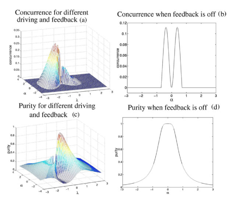
Figure 2: Plot of concurrence and purity vs driving and feedback amplitude.

Fig. 2 is the plot of concurrence and purity vs driving and feedback amplitude. As shown in Fig.2 a2, we can get certain amount of entanglement in the steady-state of a unmodulated driving system thesis1 . In this case the maximum concurrence is about 0.11, with appropriate choice of the driving amplitude $\alpha=0.38\gamma^{-1}$. The steady state is independent of the initial state as long as it is in the symmetric subspace, such as $|{g}\rangle\langle{g}|$. The coherent evolution alone is not able to produce any entanglement for an initially unentangled state, as it only consists of single qubit rotation with no coupling between two qubits. Therefore the steady-state entanglement is due to the common cooperative decoherence coupling to the cavity environment acting together with the coherent evolution thesis1 .

After including feedback onto the amplitude of the driving on the atom, proportional to the homodyne photocurrent, we see that feedback is remarkable as the steady-state concurrence has been improved from $0.11$ to $0.31$ as shown in Fig.2 a1, with appropriate choice of driving amplitude $\alpha=\pm{0.4}{\gamma^{-1}}$ and feedback amplitude $\beta=-0.8\gamma^{-1}$.

The gain of the steady state entanglement comes at the price of a loss of purity, as shown in Fig. 2 (b). There are a number of measures that can be used for the degree of purity, for example, the von Neumann entropy given by $S=-\rm Tr[{\rho}\ln{\rho}]$, and the trace sqared of the density matrix. In this paper we choose the measure of purity given by

$$r^{2}=\frac{4}{3}(\rm Tr[{{\rho}}^{2}]-\frac{1}{4}).$$ (39)

From the above equations, we find that

$$r^{2} = \frac{1}{9}+\frac{8}{9}\big{[}x_{12}^{2}+x_{13}^{2}+x_{23}^{2}+y_{12}^{2}+y_{13}^{2}+x_{23}^{2}+z_{12}^{2}$$ (40)

$$+\frac{1}{3}(2z_{13}-z_{12})^{2}\big{]}.$$

The minimum purity in $3\times 3$ subspace is obviously $\frac{1}{9}$. Note that Eq(36) measure is linear in $\rm Tr[{{\rho}}^{2}]$ with minimum $0$ and maximum $1$. The minimum of $0$ is only attainable in $4\times 4$ Hilbert space.

To gain further insight into the purity of the steady-state when it is entangled, we may look at the position of the steady-state located in the concurrence-purity plane. We begin by choosing a series of driving and feedback amplitudes, and determine their corresponding purity and entanglement. In Fig.3, we display these results with dots, representing the case of feedback-modulated driving, and stars,representing the case of unmodulated driving. Obviously, the feedback mechanism leads to a noticeable increase of entanglement, though it results in a less pure state. The continuous curve in Fig.3 represents the maximally-entangled mixed states, states with the maximal amount of entanglement for a given degree of purity, or in other words, states with the minimum purity for a given concurrence. The concurrence and the purity of a maximally entangled mixed state satisfy the following equation munro

$$r^{2}={1-\frac{3}{4}[4g(2-3g)-C^{2}]},$$ (41)

where

$$g=\left\{\begin{array}[]{cc}{C}/{2}&~{}~{}~{}~{}{\rm for}~{}~{}C>{2}/{3}\\ {1}/{3}&~{}~{}~{}~{}{\rm for}~{}~{}C<{2}/{3}\end{array}\right.$$

In reference munro , the degree of the mixture of a state is defined by linear entropy $S_{L}$. The purity $r^{2}$ defined in this paper is related to $S_{L}$ by $r^{2}=1-S_{L}$.

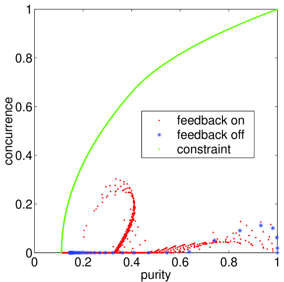
Figure 3: Plot of concurrence vs purity. The dots representing the case of feedback-modulated driving laser with two adjustable parameters $\alpha$ and $\lambda$, and the stars the case of unmodulated driving only with one adjustable parameter $\alpha$. The continuous diagonal curve tands for the maximally-entangled mixed states, states with the maximal amount of entanglement for a given degree of purity

IV Q function and density matrix

To gain further knowledge about the nature of the steady-state when it is maximally entangled, we look at the density matrix and $Q$ function. Since the density matrix elements are complex numbers, we plot in Fig.4 the modulus of the matrix elements. We use the unentangled basis states

$$|{\psi_{1}}\rangle = |{g}\rangle_{1}|{g}\rangle_{2},$$ (42)

$$|{\psi_{2}}\rangle = |{g}\rangle_{1}|{e}\rangle_{2},$$

$$|{\psi_{3}}\rangle = |{e}\rangle_{1}|{g}\rangle_{2},$$

$$|{\psi_{4}}\rangle = |{e}\rangle_{1}|{e}\rangle_{2}.$$

because a separable basis is needed to discuss entanglement.

To define the $Q$ function we need atomic coherent state $|{\zeta}\rangle$  arecchi ; radcliffe

$$|{\zeta}\rangle=(1+{|(\zeta)}|^{2})^{-j}\exp[{\zeta}\hat{J^{+}}]|{j,-j}\rangle.$$ (43)

The atomic coherent state is the closest quantum mechanical states to a classical description of a spin system.

The $Q$ function is a positive distribution function, which is defined as

$$Q(\theta,\phi) = {\langle}j,\theta,\phi|\rho|j,\theta,\phi{\rangle}$$

$$|j,\theta,\phi{\rangle} = \sqrt{\frac{(2j)!}{(j+m)!(j-m)!}}$$

$$\sum_{m=-j}^{j}\left[\cos^{j+m}(\frac{\theta}{2})\sin^{j-m}(\frac{\theta}{2})e^{-im{\phi}}\right]|j,m{\rangle},$$

where the state $|j,\theta,\phi{\rangle}$ is the spherical representation of the coherent state $|{\zeta}\rangle$ where $\theta$ and $\phi$ are the standard spherical polar coordinates defined by $\zeta=\rm arctan{\frac{\theta}{2}}{e^{-i\phi}}$. The magnitude of the $Q$ function in a particular direction ($\theta$ and $\phi$) is represented in Fig.4 by the distance measured from the origin. Since the $Q$ function is the projection of the density matrix into a coherent state , the $Q$ function does not give more information than the density matrix. However, the advantage of the $Q$ function is that it gives a more intuitive view of where the state is located.

We plot the steady-state $Q$ function and density matrix in Fig.4. There are a number of points that need explanation. First, when there is only the unmodulated driving laser shining on the system, the steady state having the most entanglement is mainly confined to the ground state $Q$ function and the upper state is almost unpopulated. However, when the driving amplitude is modified by feedback, the upper state becomes very well populated and the entanglement is greatly increased. This is not surprising, as more population in the upper state enhances nonlinearity both in the decoherence coupling and *coherent* evolution of the two-qubit system.

Second, in the particular separable $4\times 4$ basis , the off-diagonal elements of the density matrix represent coherence and the presence of coherence is a necessary condition for the creation of entanglement. To illustrate this, we plot three Bell states which are the maximally entangled states in Fig.4. We see that the off-diagonal terms are present in these maximally entangled states. In contrast, we also plot three non-entangled states, the identity, the ground state and the excited state. We see that none of the off-diagonal elements appear.

Third, when there is only the unmodulated driving laser shining on the system, the density matrix of the most entangled steady-state looks most similar to that of superposition of $|{gg}\rangle$ and some of a Bell state $\frac{1}{\sqrt{2}}(|{eg}\rangle+|{ge}\rangle)$, while when the feedback modulation is switched on, the steady-state density matrix looks more like a mixture of a non-maximally entangled state $a|{eg}\rangle+b|{ge}\rangle$ and $|{ee}\rangle+|{gg}\rangle$.

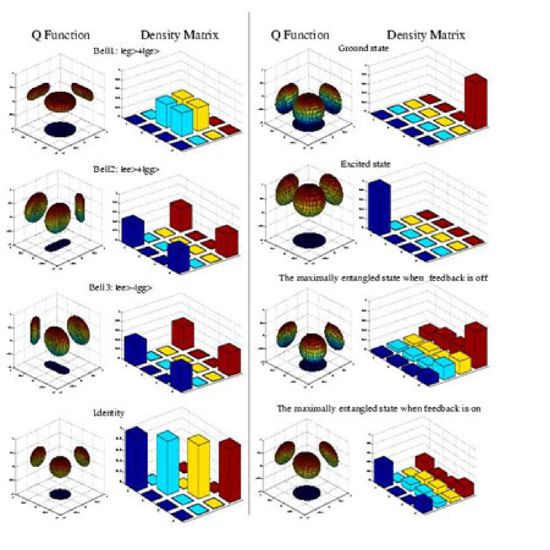
Figure 4: Plots of the $Q$ function and its projections on each of three planes, and the absolute values of matrix elements of the density matrix are shown for each of eight different states, as indicated in the figure. The magnitude of the $Q$ function in a particular direction is represented by the distance measured from the center of the $Q$ function.The diagonal elements of the density matrix are $|{ee}\rangle\langle{ee}|,|{eg}\rangle\langle{eg}|,|{ge}\rangle\langle{ge}|,|{gg}\rangle\langle{gg}|$ from left to right respectively.

V Discussion

To summarize, entanglement between two qubits can be created dynamically by driving and coupling them to a heavily damped cavity mode. When there is only the unmodulated driving laser shining on the system, the maximum steady-state concurrence (a measure of entanglement) is 0.11 thesis1 . In this paper we have re-derived these results and constructed a scheme to increase the steady state entanglement by using homodyne-mediated feedback, in which the driving laser is modulated by the homodyne photocurrent derived from the cavity output.

An analytical form for the steady-state solution of the master equation with feedback was derived and was used to show that the amount of the maximum steady-state concurrence has been increased from 0.11 to 0.31. The properties of the entangled state were also studied through the discussion of the $Q$ function and the density matrix. The important point here is that the feedback scheme can lift the steady-state from the ground state towards the excited state. Indeed with such a feedback scheme the most entangled state much closer to the Bell states, which are maximally entangled states. The details about how the feedback mechanism dynamically changes the position of the steady-state when it is maximally entangled are still largely unknown and require further investigation. Open questions such as “can the most entangled steady-state be realized experimentally?”, “what happens if individual decay of each atom cannot be ignored in the calculation”, “how does one increase both entanglement and the purity of a mixed state”, “to what extent can the system be treated semi-classically” and “what happens for a higher number of atoms” are subjects for future exploration.

VI Acknowledgments

Jin Wang would like to acknowledge stimulating discussions with Dr. Herman Batelaan, Dr. Hong Gao, Dr. Mikhail Frolov, Andrei Y. Istomin, Amiran Khuskivadze, and Dr. Anthony Starace as well as support from the Nebraska Research Initiative on Quantum Information. Jin Wang would also like to thank Jeremy Podany for proofreading. H. M. Wiseman and G. J. Milburn would like to acknowledge the support of the Australian Research Council Special and the State of Queensland.

References

- (1) C. H. Bennett, G. Brassard, C. crepeau, R. Josza, A. Peres, and W. K. Wootters, Phys. Rev. Lett. 70, 1895 (1993)
- (2) D. Vitali, M Fortunato and P. Tombesi, Phys. Rev. Lett. 85, 445, (2000)
- (3) R.F. Werner, All Teleportation and Dense Coding Schemes, quantph/0003070
- (4) W. T. Buttler, et al, Phys. Rev. Lett. 81, 3283, (1998).
- (5) P. shor and J. Preskill, Phys. Rev. Lett 85, 441, (2000).
- (6) H.K. Lo, S.Popescu, and T.P.Spiller editors, Introduction to Quantum Computing and Information, World Scientific (1998).
- (7) W.J. Munro, D.F.V.James, A.G. White, and P. G. Kwiat, Phys. Rev. A 64, 030302 (2001).
- (8) Richard Jozsa, Daniel S. Abrams, Jonathan P. Dowling, Colin P. Williams, Physical Review Letters 85, 2010-2013, quant-ph/0004105,2000
- (9) V. Vedral, M. B. Plenio, M. A. Rippen, and P. L. Knight, Phys. rev. Lett, 78, 2275 (1997).
- (10) W. Wootters, Phys. Rev. Lett. 80, 2245, (1998).
- (11) E.M. Rains, Phys. Rev. A 60, 173, (1999).
- (12) J. von Neumann, Mathematical Foundations of Quantum Mechanics. (Princeton University Press, Princeton, 1955).
- (13) J. Eisert and M. Plenio, J. Mod. Opt. 46,145 (1999)
- (14) K. Zyczkowski, Phys. Rev. A 60,3496 (1999).
- (15) S.Schneider, G. J. Milburn Phys. Rev A 65, 042107, 2002.
- (16) Y.Yamamoto, N. Imoto and S. Machida, Phys Rev. A 33, 3243 (1986)
- (17) J. M. Shapiro et al J. Opt. Soc. Am. B 4, 1604 (1987)
- (18) H. M. Wiseman and G. J. Milburn, Phys. Rev. A 47, 642 (1993).
- (19) Ozgur Cakir, Alexander A Klyachko, Alexander S Shumovsky, http://arXiv.org/abs/quant-ph/0406081, (2004).
- (20) H. J. Carmichael, An Open Systems Approach to Quantum Optics (Springer-Verlag, Berlin, 1993).
- (21) C.W. Gardiner, Handbook of Stochastic Methods (Springer, Berlin, 1985).
- (22) Proceedings of the symposium “One Hundred Years of the Quantum: From Max Planck to Entanglement,” University of Puget Sound, October 29-30, 2000, eds. J. Evans and A. Thorndyke (University of Chicago Press, to be published)
- (23) H. M. Wiseman and G. J. Milburn, Phys. Rev. A 47, 1652 (1993).
- (24) R. Bonifacio (editor) Dissipative systems in quantum optics : resonance fluorescence, optical bistability, superfluorescence Springer-Verlag, Berlin, 1982
- (25) F. T. E. Courtens, R. Gilmore and H. Thomas, Phys. Rev A 6, 2211 (1972).
- (26) Radcliffe, J. M., J. Phys. A 4, 313, (1971).