Position and Momentum Entanglement of Dipole-Dipole Interacting Atoms in Optical Lattices: The Einstein-Podolsky-Rosen Paradox on a Lattice

Abstract

We study a possible realization of the position- and momentum-correlated atomic pairs that are confined to adjacent sites of two mutually shifted optical lattices and are entangled via laser-induced dipole-dipole interactions. The Einstein-Podolsky-Rosen (EPR) “paradox” [Phys. Rev. 47, 777 (1935)] with translational variables is then modified by lattice-diffraction effects. This “paradox” can be verified to a high degree of accuracy in this scheme.

I INTRODUCTION

Einstein, Podolsky and Rosen (EPR) EPR put forth the question of whether the quantum mechanical description of physical reality is complete, giving the example of a two-particle quantum state showing peculiar correlations (dubbed “entanglement” or “Verschränkung” by Schrödinger sch ): if one measures the position or momentum of one particle, one can predict with certainty the outcome of measuring their counterpart for the other particle. Thus, depending on which measurement is chosen for the first particle, the value of either the position or momentum can be predicted with arbitrary precision for the second particle. The ensuing controversy has revolved around the interpretation of the EPR problem and its implications on quantum theory Bohr . Later, Bohm considered Boh two entangled spin-1/2 particles, which have become the focus of attention on this EPR issue: their discrete-variable entangled states have served to demonstrate the incompatibility of quantum mechanics with local realism, by the violation of Bell’s inequality Bell64 ; CHSH69 ; Aspect82a ; Aspect82 ; Perrie85 ; OuMandel ; Tittel ; Weihs ; Rowe ; Rauch . In recent years, there has been revival of interest in continuous-variable entanglement, in the spirit of the original EPR problem Gisin91 ; GisinPeres92 ; Reid ; Ou ; Silberhorn01 ; BraunsteinKimble ; Furusawa98 ; Silberhorn02 ; Polzik ; PolzikNature ; LloydSlotine98 ; Braunstein98 ; Braunstein98N ; LloydBraunstein99 ; Parkins ; ZhangBraunstein ; opa01 ; PRL03 .

The original ideal EPR EPR state of two particles—1 and 2, is, respectively, represented as follows in their coordinates or momenta (in one dimension),

$$\langle x_{1},x_{2}|\psi_{\rm EPR}\rangle = \delta(x_{1}-x_{2}),$$

$$\langle p_{1},p_{2}|\psi_{\rm EPR}\rangle = \delta(p_{1}+p_{2}).$$ (1)

If two particles are prepared in such a state, and one measures the value of $x_{1}$ (or $p_{1}$) of particle 1, one can predict the result of measuring $x_{2}$ (or $p_{2}$, respectively) with perfect precision. The state of Eq. (1) would, however, occupy infinite space and have infinite kinetic energy. One can consider more realistic variants of this state, e.g., a Gaussian state given by

$$\langle x_{1},x_{2}|\psi_{\rm EPR}\rangle = \frac{1}{\sqrt{\pi\Delta x_{-}\Delta x_{+}}}\exp\left(-\frac{(x_{1}-x_{2})^{2}}{4\Delta x_{-}^{2}}\right)\exp\left(-\frac{(x_{1}+x_{2})^{2}}{4\Delta x_{+}^{2}}\right),$$

$$\langle p_{1},p_{2}|\psi_{\rm EPR}\rangle = \frac{1}{\sqrt{\pi\Delta p_{-}\Delta p_{+}}}\exp\left(-\frac{(p_{1}-p_{2})^{2}}{4\Delta p_{-}^{2}}\right)\exp\left(-\frac{(p_{1}+p_{2})^{2}}{4\Delta p_{+}^{2}}\right),$$ (2)

where $\Delta p_{\pm}\equiv\hbar/\Delta x_{\pm}$ (see Fig. 1). The original EPR state corresponds to the limit $\Delta x_{-}/\Delta x_{+}\to 0$. After measuring the position of particle 1, the position of particle 2 is centered at

$$\bar{x}_{2}=x_{1}\frac{1-\left(\frac{\Delta x_{-}}{\Delta x_{+}}\right)^{2}}{1+\left(\frac{\Delta x_{-}}{\Delta x_{+}}\right)^{2}},$$ (3)

with the uncertainty $\Delta x_{-}\left[1+\left(\frac{\Delta x_{-}}{\Delta x_{+}}\right)^{2}\right]^{-1/2}$. In the limit of $\Delta x_{-}/\Delta x_{+}\ll 1$, the position of particle 2 is centered at $x_{1}$, and its uncertainty is $\approx\Delta x_{-}$. Similar relations hold also for the momentum of particle 2 after the momentum of particle 1 is measured. Thus, either of the two conjugate quantities of particle 2 can be predicted with arbitrarily high precision. Of course, the Heisenberg uncertainty relation is not violated, since for a single system one can measure only one of the two conjugate quantities.

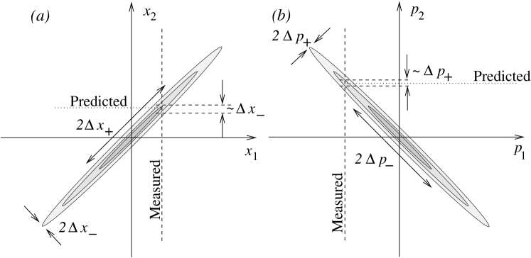
Figure 1: Joint probability distribution of positions $(a)$ and of momenta $(b)$ of EPR-pair ensembles. If one measures the position of particle 1, one can predict the position of particle 2 with uncertainty $\approx\Delta x_{-}$, whereas if one measures momentum of particle 1, one can predict the momentum of particle 2 with uncertainty $\approx\Delta p_{+}$.

Approximate versions of the translational EPR state, wherein the $\delta$-function correlations are replaced by finite-width distributions, have been shown to characterize the quadratures of the two optical-field outputs of parametric downconversion Reid ; Ou , or of a fiber interferometer with Kerr nonlinearity Silberhorn01 . Such states allow for various schemes of continuous-variable quantum information processing such as quantum teleportation BraunsteinKimble ; Furusawa98 or quantum cryptography Silberhorn02 . A similar state has also been predicted and realized using collective spins of large atomic samples Polzik ; PolzikNature . It has been shown that if suitable interaction schemes can be realized, continuous-variable quantum states of the original EPR type could even serve for quantum computation Braunstein98 ; Braunstein98N ; LloydSlotine98 ; LloydBraunstein99 .

Notwithstanding its applications to quantum information processing, the translational EPR state of Eq. (2) does not entail a violation of local realism: such a state has a non-negative Wigner function, controlling the position and momentum distribution of each particle. Nevertheless, there exist measurement schemes in which an analog of Bell’s inequality is violated Gisin91 ; GisinPeres92 for such a state—as for any pure entangled state.

The realization and measurement of the EPR translational correlations of material particles appears to be very difficult. There have been suggestions to start with entangled light fields and to transfer their quantum state into the state of trapped ions in optical cavities Parkins or of vibrating mirrors ZhangBraunstein . We have proposed to realize translational EPR states by taking advantage of interatom correlations in a dissociating diatom opa01 . More recently, we have considered dipole-dipole coupled cold atoms in an optical lattice as a source of translational EPR states PRL03 .

In order to generate the translational EPR entanglement between interacting material particles, one must be able to accomplish several challenging tasks: (a) switch on and off the entangling interaction; (b) confine their motion to single dimension, and (c) infer and verify the dynamical variables of particle 2 at the time of measurement of particle 1. The latter requirement is particularly hard for free particles, since by the time we complete the prediction for particle 2, its position will have changed. In opa01 we suggested to overcome these hurdles by transforming the wavefunction of flying (ionized) atoms emerging from diatom dissociation by an electrostatic/magnetic lens onto the image plane, where its position corresponds to what it was at the time of the diatom dissociation. In PRL03 we have proposed a solution based on the following steps: (i) controlling the diatom formation and dissociation in an optical lattice by switching on and off a laser-induced dipole-dipole interaction; (ii) controlling the motion and effective masses of the atoms and the diatom by changing the intensities of the lattice fields. In this article we discuss our proposal in more detail and elaborate on its principles.

Our aim here is to demonstrate the feasibility of preparing a momentum- and position-entangled state of atom pairs in optical lattices, which would be a variant of the original EPR state, owing to lattice diffraction. In Sec. II we specify the physical system under study. In Sec. III the basic properties of single-atom states in optical lattices are discussed. In Sec. IV we discuss the binding effect of the dipole-dipole interaction. Sec. V deals with the preparation of EPR states by manipulation of the effective masses of the atoms. In Sec. VI we discuss experimental demonstration possibilities of measuring the EPR Sec. VII is devoted to conclusions.

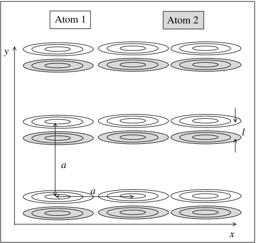
Figure 2: Proposed scheme of overlapping optical lattices used to prepare the translational EPR state. The lattices are displaced from each other in the $y$ direction by $l$. They are sparsely occupied by two kinds of atoms. Each of the two kinds of atoms feels a different lattice; the shaded regions depict the energy minima (potential wells) of the lattices.

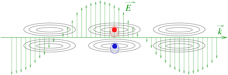
Figure 3: Scheme of the LIDDI interaction: a traveling laser field propagating in the direction $x$ along which the atoms are weakly confined. The electric field vector is in the $xy$ plane. The field induces dipole moments in the atoms, thereby causing the interatomic interaction.

II System description

Let us assume two overlapping optical lattices with the same lattice constant $a$, as in Fig. 2. The lattices are very sparsely occupied by two kinds of atoms, each kind interacting with only one of the two lattices. This can be realized, e.g., by assuming two different internal (say, hyperfine) states of the atoms Brennen . In both lattices, the potentials are strongly confining in the $y$ and $z$ directions (realized by strong laser fields), whereas in the $x$ direction the lattice potential is only moderately to weakly confining. Thus, the motion of each particle is restricted to the $x$ direction. In each direction we assume that only the lowest vibrational energy band is occupied. Initially, the potential minima of the lattices are displaced from each other by an amount $l\ll a$ in the $y$ direction. An auxiliary laser produces a laser-induced dipole-dipole interaction (LIDDI) between the atom pairs. It is linearly polarized in the $y$ direction, traveling in the $x$ direction and has a wavelength $\lambda_{\rm C}$, moderately detuned from an atomic transition that differs from the transition used to trap the atoms in the lattice. In the case of two atoms with identical polarizabilities in the geometry of Fig. 3, the interatomic LDDI potential induced by a linearly polarized laser is of the form Thirun

$$V_{\rm dd}=-V_{\rm C}F_{\theta}(kR),$$ (4)

where

$$F_{\theta}(kR)=\cos\left(kR\cos\theta\right)\left\{(2\!-\!3\cos^{2}\theta)\left[\frac{\cos kR}{(kR)^{3}}\!+\!\frac{\sin kR}{(kR)^{2}}\right]\!+\!\cos^{2}\theta\frac{\cos kR}{kR}\right\},$$ (5)

and

$$V_{\rm C}=\frac{\alpha^{2}k^{3}I_{\rm C}}{4\pi\epsilon_{0}^{2}c}.$$ (6)

Here the wavenumber is $k=2\pi/\lambda_{\rm C}$, $I_{\rm C}$ is the coupling laser intensity, and the atomic dynamic polarizability $\alpha$ is

$$\alpha=\frac{2\omega_{A}|\mu|^{2}}{\hbar(\omega_{A}^{2}-\omega^{2})},$$ (7)

$\mu$ being the dipole moment element, $\omega_{A}$ the atomic transition frequency, and $\omega=kc$. The position-dependent part $F_{\theta}(kR)$ is a function of $R$, the distance between the atoms, and $\theta$, the angle between the interatomic axis and the wavevector of the coupling laser. Since $l\ll 2a$, $V_{\rm dd}(R)$ has a pronounced minimum for atoms located at the nearest sites, $R\simeq l$, where

$$V_{\rm dd}(R)\simeq-\frac{V_{\rm C}}{4\pi^{3}}\left(\frac{\lambda_{\rm C}}{l}\right)^{3}.$$ (8)

The LIDDI energy as a function of $l$ and the relative position of the atoms is shown in Figs. 4 and 5. Under the above assumptions, we can treat the system as consisting of pairs of “tubes”, either empty or occupied, that are oriented along $x$. Only atoms within adjacent tubes are appreciably attracted to each other along $y$, due to the LIDDI.

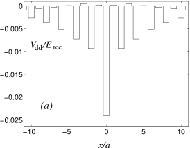
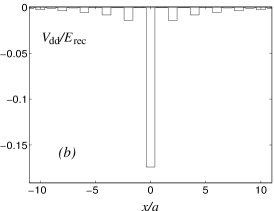
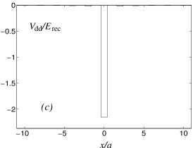
Figure 4: LIDDI potential as a function of the position of atom 2, given that atom 1 occupies site 0, for different separations of the two lattices: (a) $l=200$ nm, (b) $l=100$ nm, (c) $l=40$ nm. The other parameters are specified in Sec. V.

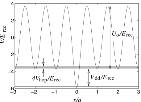
Figure 5: Position dependence of the potential energy of atom 2, given that atom 1 is located at site 0. The horizontal lines denote the lowest band of energies corresponding to uncorrelated atoms (bandwidth $4V_{\rm hop}$) and the band of diatom energies $V_{\rm dd}$ (below the band of uncorrelated atoms).

III Single-atom states in the Wannier basis

Let us focus on the subensemble of tube-pairs in which each tube is occupied by exactly one atom. In the 1D optical lattice, the single-atom Hamiltonian is

$$\hat{H}_{\rm lat}=\frac{U_{0}}{2}\cos\left(\frac{2\pi x}{a}\right)+\frac{\hat{p}_{x}^{2}}{2m}.$$ (9)

Here $m$ is the atomic mass, $\hat{p}_{x}$ is the momentum operator, $U_{0}$ is the maximum potential energy due to the interaction of the atomic dipole with the laser field,

$$U_{0}=\frac{4|\mu_{L}|^{2}}{\epsilon_{0}\hbar c\delta_{L}}I_{L},$$ (10)

where $\mu_{L}$ is the dipole matrix element of the lattice transition, $\delta_{L}$ is the detuning of the lattice field from this transition, and $I_{L}$ is the intensity of the lattice field. The Hamiltonian (9) describes a quantum pendulum. The eigenfunctions of the corresponding Schrödinger equation are the Mathieu functions Slater . The eigenvalues form bands, whose spectrum depends on the ratio of $U_{0}$ to the recoil energy,

$$E_{\rm rec}=\frac{2\pi^{2}\hbar^{2}}{m\lambda_{\rm L}^{2}},$$ (11)

so that one can distinguish between strongly binding ($U_{0}\gg E_{\rm rec}$) and weakly binding ($U_{0}\sim E_{\rm rec}$) potentials. We assume that the atoms are cooled down to the lowest energy band of the lattice, in the absence of LIDDI.

The state of each atom is then conveniently described in terms of Wannier functions $|\chi_{j}\rangle$ Wannier that are localized at lattice sites labeled by index $j$. The Wannier functions are superpositions of the delocalized Bloch eigenfunctions $|\phi_{k}\rangle$ of the same band,

$$|\chi_{j}\rangle=\frac{1}{\sqrt{N}}\sum_{k}\exp\left(-ikx_{j}\right)|\phi_{k}\rangle,$$ (12)

where $N$ is the number of lattice sites, and $x_{j}$ is the position of the $j$th site. Since the Wannier functions are not eigenfunctions of the single-particle Hamiltonian, an atom initially prepared in a Wannier state that is localized at one site, will subsequently tunnel to the neighboring sites. Nevertheless, if the tunneling rate is sufficiently slow, the single-particle Hamiltonian (9) in the Wannier basis has a relatively simple form:

$$H_{\rm lat}\approx\left(\begin{array}[]{cccccc}\dots&\dots&\dots&\dots&\dots&\dots\\ \dots&H_{0}&V_{\rm hop}&0&0&\dots\\ \dots&V_{\rm hop}&H_{0}&V_{\rm hop}&0&\dots\\ \dots&0&V_{\rm hop}&H_{0}&V_{\rm hop}&\dots\\ \dots&0&0&V_{\rm hop}&H_{0}&\dots\\ \dots&\dots&\dots&\dots&\dots&\dots\\ \end{array}\right).$$ (19)

Here the diagonal elements $H_{0}$ are equal to the energy at the center of the band, and only two sets of off-diagonal elements, expressing hopping between the neighboring sites, are non-negligible:

$$H_{0}=\langle\chi_{j}|\hat{H}_{\rm lat}|\chi_{j}\rangle,\ \ V_{\rm hop}=\langle\chi_{j}|\hat{H}_{\rm lat}|\chi_{j+1}\rangle,$$ (20)

The hopping rate is related to the energy bandwidth of the lowest lattice band $V_{B}$ by $V_{B}\approx 4|V_{\rm hop}|$ (for exact expressions see Slater ).

For a moderately deep lattice potential ($U_{0}\lesssim 15E_{\rm rec}$), the quantum-pendulum Schrödinger equation yields the approximate formulae for $V_{\rm hop}$ and the single-atom effective mass:

$$V_{\rm hop} \approx \frac{1}{4}E_{\rm rec}\exp\left(-0.26\frac{U_{0}}{E_{\rm rec}}\right),$$ (21)

$$m_{\rm eff} = \frac{2\hbar^{2}}{a^{2}V_{B}}\approx\frac{\hbar^{2}}{2a^{2}|V_{\rm hop}|}$$ (22)

The Wannier functions of the lowest band can be approximated by Gaussians:

$$\langle x|\chi_{j}\rangle\approx\langle x|\psi_{j}^{\rm Gauss}\rangle=\frac{1}{\sqrt{2\pi\sqrt{\sigma_{G}}}}\exp\left(-\frac{(x-x_{j})^{2}}{4\sigma_{G}^{2}}\right),$$ (23)

where

$$\sigma_{G}^{2}=\frac{\lambda_{L}^{2}}{4\pi^{2}}\sqrt{\frac{E_{\rm rec}}{2U_{0}}}.$$ (24)

This approximation is relatively accurate for $U_{0}\gtrsim 6E_{\rm rec}$ (see the inset in Fig. 11) with fidelity $|\langle\psi_{j}^{\rm Gauss}|\chi_{j}\rangle|^{2}>98$%. Note, however, that the Gaussian approximation is not suitable for calculating the hopping potential (20) since this quantity is very sensitive to the non-Gaussian tails of the Wannier wavefunctions.

IV Diatom binding and translational EPR states

Let us now assume that two neighboring tubes in Fig. 3 are occupied by one atom each and the LIDDI is turned on. If the tubes are close to each other ($l\ll\lambda_{\rm C}$, as in Fig. 4), the interaction Hamiltonian in the Wannier basis has nonzero elements only for atoms residing at the nearest sites,

$$\hat{H}_{\rm int}\approx V_{\rm dd}\sum_{j}|\chi_{j}^{(1)}\rangle|\chi_{j}^{(2)}\rangle\langle\chi_{j}^{(1)}|\langle\chi_{j}^{(2)}|,$$ (25)

and the total two-atom Hamiltonian is

$$\hat{H}^{\rm(2at)}=\hat{H}_{\rm lat}^{(1)}\otimes\hat{1}^{(2)}+\hat{1}^{(1)}\otimes\hat{H}_{\rm lat}^{(2)}+\hat{H}_{\rm int}.$$ (26)

This Hamiltonian has been diagonalized numerically, and its eigenvalues are shown in Fig. 6 as a function of the hopping and binding potential strength. One can see that for a sufficiently large ratio $|V_{\rm dd}|/|V_{\rm hop}|$ a band of diatomic states is split off the band of independent atoms, towards lower energies.

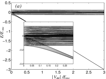
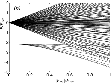
Figure 6: Eigenvalues of the two-atom Hamiltonian as a function of $(a)$ the dipole-dipole coupling $V_{\rm dd}$ (for a constant hopping potential $|V_{\rm hop}|=0.0355~{}E_{\rm rec}$), and $(b)$ the hopping potential $V_{\rm hop}$ (for a constant dipole-dipole coupling potential $V_{\rm dd}=2.16~{}E_{\rm rec}$).

For a strong LIDDI binding, $|V_{\rm hop}|\ll|V_{\rm dd}|$, the ground state of the Hamiltonian (26) corresponds to a tightly bound diatom which can be approximated by

$$|\psi_{0}\rangle\approx\frac{1}{\sqrt{N}}\sum_{j}|\chi_{j}^{(1)}\rangle|\chi_{j}^{(2)}\rangle.$$ (27)

This is a highly correlated state: when particle 1 is found at the $j$th site of lattice 1, then particle 2 is found at the $j$th site of lattice 2, with position dispersion given by the half-width $\sigma$ of the atomic Wannier function in the lowest band, $\sigma\approx\sigma_{G}$ (Fig. 7a). The Fourier transform of this wave function yields its momentum representation. The corresponding momentum probability distribution exhibits anti-correlation similarly to the EPR states (1) or (2), but it reflects the lattice periodicity (Fig. 8a). In momentum space, the state occupies a region of half-width $\hbar/(2\sigma)$, and the probability distribution has narrow ridges along $p_{2}=-p_{1}$. The width of the ridges is inversely proportional to the lattice size, $\Delta p_{+}\sim\hbar/(Na)$, and they are shifted by $2\pi\hbar/a$ from each other.

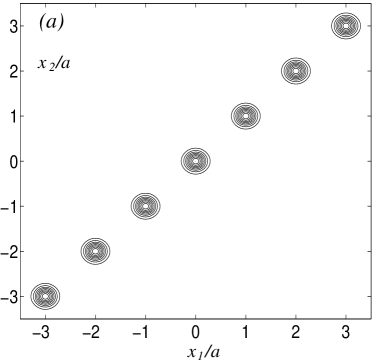
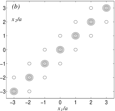
Figure 7: Joint probability distribution of the positions of two atoms in the ground state of Hamiltonian (26) for $|V_{\rm hop}|=0.0355E_{\rm rec}$: $(a)$ $|V_{\rm dd}|=1.0E_{\rm rec}$, $(b)$ $|V_{\rm dd}|=0.10E_{\rm rec}$.

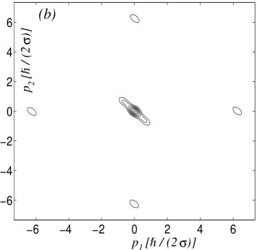
Figure 8: Joint probability distribution of the momenta of two atoms in the ground state of Hamiltonian (26) for $|V_{\rm hop}|=0.0355E_{\rm rec}$: $(a)$ $|V_{\rm dd}|=1.0E_{\rm rec}$, $(b)$ $|V_{\rm dd}|=0.10E_{\rm rec}$.

The probability of atoms to escape their EPR partners “over the next” sites increases with the ratio $V_{\rm hop}/V_{\rm dd}$. This leads to an increase of the position dispersion which can be estimated by first-order perturbation theory: Let atoms 1 and 2 occupy the $j$th site in the absence of $V_{\rm hop}$. With the perturbation $V_{\rm hop}$ on, atom 2 can occupy also sites $j\pm 1$, which have energies $|V_{\rm dd}|$ above the unperturbed state, with the probability $\approx|V_{\rm hop}|^{2}/|V_{\rm dd}|^{2}$. This contributes to an increase in the diatomic separation dispersion,

$$\Delta x_{-}^{2}\approx\sigma^{2}+2a^{2}\left(\frac{V_{\rm hop}}{V_{\rm dd}}\right)^{2},$$ (28)

resulting in the joint probability distribution of the atomic positions and momenta as a function of $V_{\rm hop}/V_{\rm dd}$, shown in Fig. 7b and Fig. 8b, respectively.

The states of the tightly bound diatom form a separate band whose bandwidth is

$$V_{B}^{\rm(2at)}\approx 4|V_{\rm hop}^{\rm(2at)}|,$$ (29)

below the lowest atomic vibrational band. The diatomic hopping potential $V_{\rm hop}^{\rm(2at)}$ can be estimated by assuming that the two atoms consecutively hop to their neighboring sites, i.e., the change

$$|\chi_{j}^{(1)}\rangle|\chi_{j}^{(2)}\rangle\to|\chi_{j+1}^{(1)}\rangle|\chi_{j+1}^{(2)}\rangle$$ (30)

is realized either via

$$|\chi_{j}^{(1)}\rangle|\chi_{j}^{(2)}\rangle\to|\chi_{j+1}^{(1)}\rangle|\chi_{j}^{(2)}\rangle\to|\chi_{j+1}^{(1)}\rangle|\chi_{j+1}^{(2)}\rangle,$$ (31)

or via

$$|\chi_{j}^{(1)}\rangle|\chi_{j}^{(2)}\rangle\to|\chi_{j}^{(1)}\rangle|\chi_{j+1}^{(2)}\rangle\to|\chi_{j+1}^{(1)}\rangle|\chi_{j+1}^{(2)}\rangle.$$ (32)

By adiabatic elimination of the higher-energy intermediate states, one obtains

$$V_{\rm hop}^{\rm(2at)}\approx 2\frac{|V_{\rm hop}|^{2}}{V_{\rm dd}}.$$ (33)

All the states of the diatomic band have correlated positions. However, the momenta are not anti-correlated in all these states in the same way as in the diatomic ground state. To realize strong momentum anti-correlations, we have to prepare a state that predominantly originates from the bottom of the diatomic band. If we work with thermal states this means that the temperature of the system must satisfy

$$k_{B}T\ll V_{B}^{\rm(2at)}.$$ (34)

Near the bottom of the band, the diatomic dynamics can be described by means of the 2-atom effective mass given by

$$m_{\rm eff}^{\rm(2at)}=\frac{2\hbar^{2}}{V_{B}^{\rm(2at)}a^{2}}\approx\frac{\hbar^{2}|V_{\rm dd}|}{4V_{\rm hop}^{2}a^{2}}.$$ (35)

The thermal (kinetic) energy of the diatom is then related to the degree of momentum anti-correlation through the sum-momentum spread $\Delta p_{+}=p_{x1}+p_{x2}$,

$$\Delta p_{+}^{2}\approx k_{B}T{2m_{\rm eff}^{\rm(2at)}}\approx\frac{\hbar^{2}|V_{\rm dd}|}{4V_{\rm hop}^{2}a^{2}}k_{B}T.$$ (36)

To determine how “strong” the EPR effect is, we compare the product of the half-widths of the position and momentum peaks in the tightly bound diatom state with the Heisenberg uncertainty limit through the parameter opa01 ; PRL03 :

$$s=\frac{\hbar}{2\Delta x_{-}\Delta p_{+}}.$$ (37)

A value of $s$ higher than 1 indicates the occurrence of the EPR effect; the higher the value of $s$, the stronger the effect.

Strictly speaking, for the multi-peak momentum distribution, one should use a more general uncertainty relation, as discussed, e.g., in Uffink , that distinguishes the uncertainty of multiple narrow peaks from that of a single broad peak. However, even the simple half-width of the peaks is a useful measure of the EPR effect. In order to maximize $s$, we must adhere to the trade-off between reducing either $\Delta x_{-}$ , by decreasing $|V_{\rm hop}/V_{\rm dd}|$, or $\Delta p_{+}$, by increasing $|V_{\rm hop}/V_{\rm dd}|$. The optimum value of $s$ generally depends on the temperature of the diatom, as detailed below.

V EPR state preparation

Cooling down the diatomic system to prepare the EPR state is a non-trivial task. We suggest a “cooling” procedure which takes advantage of the difference between the single-atom and the diatom bandwidths, and of the possibility to change the light-induced potentials. The key is first to cool down individual atoms and then separate the unpaired atoms from the diatoms. The scheme consists of three steps:

(i) We first switch on only an external, shallow, harmonic potential in the $x$ direction (all other potentials being off), and cool the $x$-motion of the atoms down to its ground state. The width $\sigma_{E}$ of the ground state should be several times the lattice constant; it is related to the desired momentum anti-correlation by $\sigma_{E}\approx\hbar/(\sqrt{2}\Delta p_{+})$. The temperature necessary to achieve this must be

$$T\ll\hbar^{2}/(4mk_{B}\sigma_{E}^{2}).$$ (38)

(ii) A weak lattice potential in the $x$-direction is then slowly switched on, so that the state becomes

$$(\sum_{j}\alpha_{j}|\chi_{j}^{(1)}\rangle)(\sum_{l}\alpha_{l}|\chi_{l}^{(2)}\rangle)=\sum_{j}\alpha_{j}^{2}|\chi_{j}^{(1)}\rangle|\chi_{j}^{(2)}\rangle+\sum_{j\neq l}\alpha_{j}\alpha_{l}|\chi_{j}^{(1)}\rangle|\chi_{l}^{(2)}\rangle,$$ (39)

where the coefficients

$$\alpha_{j}\sim\exp[-(j-j_{0})^{2}a^{2}/(4\sigma_{E}^{2})]$$ (40)

are Gaussians localized around the minimum of the external potential.

(iii) We switch on the LIDDI and change the external potential, from an attractive well to a repulsive linear potential, acting to remove the particles from the lattice. The two parts of the wavefunction (39) will respond differently: The motion of the paired atoms (corresponding to $\sum_{j}\alpha_{j}^{2}|\chi_{j}^{(1)}\rangle|\chi_{j}^{(2)}\rangle$) will remain in the vicinity of the initial position because of their narrow energy band (Fig. 9). Single (unpaired) atoms, whose bandwidth is substantially larger, will travel a much longer distance before hitting the top of the energy band. Thus, after a properly chosen time, the unpaired atoms could be removed from the $x$-region of interest, which is $\approx V_{\rm hop}/V^{(2)}_{\rm hop}$ longer for single atoms than for diatoms [see Eq.  (29)].

Provided the time $t_{c}$ is short enough for the system to remain near the bottom of these two bands, the dynamics can be interpreted in terms of the appropriate effective masses: the “heavy” diatoms with mass move much slower than the “light” single atoms with mass (22). Thus, after changing the sign of the external potential, the unpaired atoms will be ejected out of the lattice and separated from the diatoms as glumes from grains.

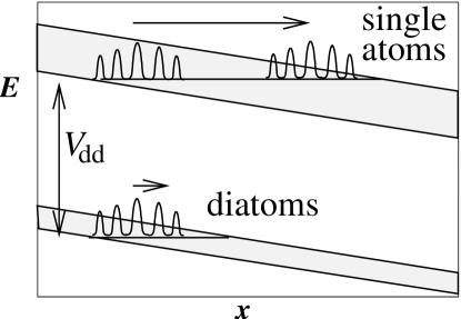
Figure 9: Separating single (unpaired) atoms from diatoms: an external repulsive potential causes both the single atoms and the diatoms to move on a surface of constant energy. The diatoms hit the top of the energy band after being displaced by a much shorter length than the unpaired atoms.

This effect is illustrated by the numerical simulation in Fig. 10 for two lithium atoms in two lattices with $\lambda_{\rm L}=$ 323 nm (corresponding to the transition 2s–3p) and a dipole-dipole coupling field of $\lambda_{\rm C}=$ 670.8 nm (transition 2s–2p). The dipole moment element of the lattice transition is $1.26\times 10^{-30}$ Cm, while the LIDDI coupling dipole element is $2.7\times 10^{-29}$ Cm. From these values we get the recoil energy $E_{\rm rec}=1.85\times 10^{-28}$J. The lattice and LIDDI field intensities are $I_{\rm L}=$ 0.186 W/cm² and $I_{\rm C}=$ 0.023 W/cm². The corresponding field detunings are $\delta_{\rm L}=50\gamma_{\rm L}$, $\delta_{\rm C}=100\gamma_{\rm C}$, the respective decay rates being $\gamma_{\rm L}=1.2\times 10^{6}$ s^-1, and $\gamma_{\rm C}=3.7\times 10^{7}$ s^-1. The two lattices are displaced by $l=$ 40 nm. From these values we get the lattice potential $U_{0}=3.93E_{\rm rec}$, the LIDDI potential of the nearest atoms $V_{\rm dd}=-0.5E_{\rm rec}$, and the hopping potential $V_{\rm hop}=-0.09E_{\rm rec}$. The two-particle hopping potential is then $V_{\rm hop}^{\rm(2at)}\approx-0.0324E_{\rm rec}$. The correlated pairs are prepared by first cooling independent atoms in an external harmonic potential with the ground-state half-width of $\sigma_{E}=5a$ (frequency of 1 kHz $\sim 30$ nK). When the linear external potential is switched on, the atoms start moving in the direction of decreasing potential energy. Figure 10, which captures the situation at three consecutive times, shows that unpaired atoms (off-diagonal peaks) are displaced by a much longer distance than the diatoms (diagonal peaks).

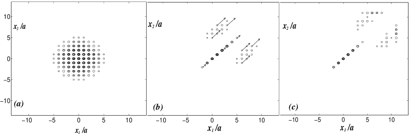
Figure 10: Simulation of the EPR state preparation in an optical lattice with 25 sites, at three consecutive times: (a) Initially ($t=0$), the atoms are cooled down to the external harmonic potential ground state, whereas the LIDDI is off. (b) At $t=1.4\times 10^{-4}$ s LIDDI and the repulsive linear potential (with the slope 0.04 $E_{\rm rec}$ per lattice site) are on, whereas the harmonic potential is off. The diatoms are moving through the lattice very slowly in comparison to the single atoms. (c) At $t=2.16\times 10^{-4}$ s single atoms are ejected out of the lattice and the diatoms are separated out.

The paired atoms remaining in the lattice are then in the state $\sim\exp[-(j-j_{0})^{2}a^{2}/(2\sigma_{0}^{2})]|\chi_{j}^{(1)}\rangle|\chi_{j}^{(2)}\rangle$ wherein positions and momenta are correlated with the uncertainties $\Delta x_{+}\approx\sigma_{E}/\sqrt{2}$ and $\Delta p_{+}\approx\hbar/\Delta x_{+}$, respectively. At higher temperatures the atoms are not cooled to the ground state of the external potential and the momentum anti-correlation has the spread

$$\Delta p_{+}\approx\hbar/\{\sqrt{2}\sigma_{E}\tanh[\hbar^{2}/(2\sigma_{E}^{2}mk_{B}T)]\}.$$ (41)

The parameter $s$ of Eq. (37) can then be estimated as

$$s\approx\frac{\sigma_{E}}{\sqrt{2}\sigma}\tanh\left[\frac{1}{\pi^{2}}\left(\frac{a}{\sigma_{E}}\right)^{2}\frac{E_{\rm rec}}{k_{B}T}\right].$$ (42)

This relation enables us to select the optimal external harmonic potential (specified here by $\sigma_{E}$) such that the parameter $s$ is maximized, for a given temperature $T$.

The small effective mass of unpaired atoms allows us to cool them to temperatures higher than that corresponding to the bottom of the diatomic band. The price is, however, that most of the atoms are discarded and only a small fraction of $\sim a/\sigma_{E}$ will remain in the bound diatom state. The different behavior of the paired and unpaired atoms in a periodic potential is a sparse-lattice analogy of the transition from Mott-insulator to a superfluid state in the fully occupied lattice, recently observed in Ref. Greiner .

The two-particle joint position distribution of the ground state is a chain of peaks of half-width $\sigma$ separated by $a$ that are located along the line $x_{2}=x_{1}$ (Fig. 11). The corresponding joint momentum distribution spreads over an area of half-width $\hbar/(2\sigma)$ and consists of ridges in the direction $p_{2}=-p_{1}$, that are separated by $2\pi\hbar/a$, and have the half-width $\pi\hbar/(Na)$ for a lattice of $N$ sites (Fig. 12).

VI Measurements

After preparing the system in the EPR state, how can one can test its properties experimentally? To this end we may increase the lattice potential $U_{0}$, switch off the field inducing the LIDDI, and separate the two lattices by changing the laser-beam angles. By increasing $U_{0}$, the atoms lose their hopping ability and their quantum state is “frozen” with a large effective mass: the bandwidth $V_{B}$ decreases exponentially with $U_{0}$ and the effective mass increases exponentially, so that the atoms become too “heavy” to move. One has then enough time to perform measurements on each atom:

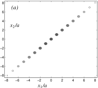
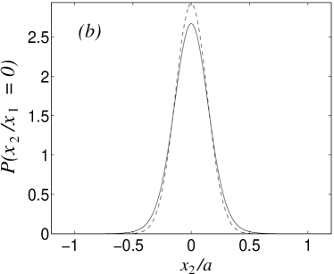
Figure 11: $(a)$ Joint probability distribution of the positions of two lithium atoms in adjacent optical lattices, prepared in a diatom state as specified in the text, using the ground state of the external harmonic potential with half-width $\sigma_{E}=6a$ and temperature of 10 nK. $(b)$ Position probability of atom 2 in the state above, conditional on atom 1 being measured at site 0 (full line). Dashed line: Gaussian approximation of the Wannier function with the half-width $\sigma=0.14a$.

a) The atomic position can be measured by detecting its resonance fluorescence. After finding the site occupied by atom 1, one can infer the position of atom 2. If this inference is confirmed in a large ensemble of measurements, it would suggest that there is an “element of reality” EPR corresponding to the position of particle 2. An example of the conditional probability of position of particle 2 after measuring the position of particle 1 is given in Fig. 11.

b) The momentum can be measured by switching off the $x$-lattice potential of the atom (thus bringing it back to its “normal” mass $m$). The distance traversed by the atom during a fixed time is proportional to its momentum. An example of the conditional probability of the momentum of particle 2 given the momentum of particle 1 is shown in Fig. 12.

c) One can test the EPR correlations between the atomic ensembles occupying the two lattices, testing large number of pairs in a single run. The correlations in $x$ and anti-correlations in $p$ would be observed by matching the distribution histograms measured on atoms from the two lattices.

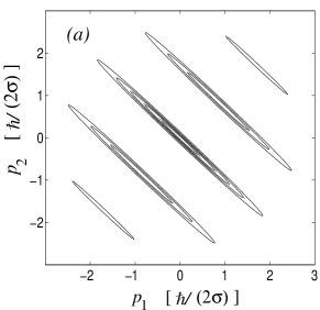
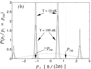
Figure 12: $(a)$ Joint probability distribution of the atomic momenta in the aforementioned state with $T=100$ nK. $(b)$ Conditional probability of the momentum of atom 2, given that the momentum of atom 1 has been measured (the measured value $p_{1}=p_{1{\rm M}}$ is indicated by an arrow)for lithium diatoms prepared as in the text. The dashed line corresponds to the marginal probability distribution of momentum $p_{2}$ irrespective of the momentum of atom 1 at the temperature $T=100$ nK. The half-width of each peak is equal to $1/s$ of Eq. (37).

VII Conclusions

We have discussed a scheme which can be used to prepare a translationally entangled pair of massive particles in a state analogous to the original EPR state EPR . A novel element of the present scheme is the extension of the EPR correlations to account for lattice-diffraction effects. Their momentum and position correlations principally differ from those of free particles [Eqs. (1), (2)]: due to the lattice periodicity, the position and momentum distributions have generally a multi-peak structure.

The realization of the proposed scheme is expected to be based on the adaptation of existing techniques (optical trapping, cooling, controlled dipole-dipole interaction). to the requirements spelled out in Sec. V and VI The most important ingredient of the scheme is the manipulation of the effective mass, for EPR-pairs preparation (by separating the “light” unpaired atoms from the “heavy” diatoms) and for their detection (by “freezing” the atoms in their initial state so that their EPR correlations are preserved long enough).

One may envision extensions of the present approach to matter teleportation opa01 and quantum computation based on continuous variables Braunstein98 ; Braunstein98N ; LloydSlotine98 ; LloydBraunstein99 . Such extensions may involve the coupling of entangled atomic ensembles in optical lattices by photons carrying quantum information.

- (1) A. Einstein, B. Podolsky, and N. Rosen, Phys. Rev. 47, 777 (1935).
- (2) E. Schrödinger, Naturwissenschaften 48, 807; ibid 49, 823; ibid 50, 844 (1935).
- (3) N. Bohr, Phys. Rev. 48, 696 (1935).
- (4) D. Bohm, Quantum Theory (Prentice-Hall, Englewood Cliffs, NJ, 1951).
- (5) J. S. Bell, Physics 1, 195 (1964).
- (6) J. F. Clauser, M. A. Horne, A. Shimony, and R. A. Holt, Phys. Rev. Lett. 23, 880 (1969).
- (7) A. Aspect, P. Grangier, and G. Roger, Phys. Rev. Lett. 49, 91 (1982).
- (8) A. Aspect, J. Dalibard, and G. Roger, Phys. Rev. Lett. 49, 1804 (1982).
- (9) W. Perrie, A.J. Duncan, H.J. Beyer, and H. Kleinpoppen, Phys. Rev. Lett. 54, 1790 (1985).
- (10) Z.Y. Ou and L. Mandel, Phys. Rev. Lett. 61, 50 (1998).
- (11) W. Tittel, J. Brendel, H. Zbinden, and N. Gisin, Phys. Rev. Lett. 81, 3563 (1998).
- (12) G. Weihs, T. Jennewein, C. Simon, H. Weinfurter, and A. Zeilinger, Phys. Rev. Lett. 81, 5039 (1998).
- (13) M.A. Rowe, D. Kielpinski, V. Meyer, C.A. Sackett, W.M. Itano, C. Monroe, and D.J. Wineland, Nature 409, 791 (2001).
- (14) Y. Hasegawa, R. Loidl, G. Badurek, M. Baron, and H. Rauch, Nature 425, 45 (2003).
- (15) N. Gisin, Phys. Lett. A 154, 201 (1991).
- (16) N. Gisin and A. Peres, Phys. Lett. A 162, 15 (1992).
- (17) M.D. Reid and P.D. Drummond, Phys. Rev. Lett. 60, 2731 (1988).
- (18) Z.Y. Ou, S.F. Pereira, H.J. Kimble, and K. C. Peng, Phys. Rev. Lett. 68, 3663 (1992).
- (19) C. Silberhorn, P.K. Lam, O. Weiss, F. König, N. Korolkova, and G. Leuchs, Phys. Rev. Lett. 86, 4267 (2001).
- (20) S.L. Braunstein and H.J. Kimble, Phys. Rev. Lett. 80, 869 (1998).
- (21) A. Furusawa, J. L. Sørensen, S. L. Braunstein, C. A. Fuchs, H. J. Kimble, and E. S. Polzik, Science 282, 706 (1998).
- (22) C. Silberhorn, N. Korolkova, and G. Leuchs, Phys. Rev. Lett. 88, 167902 (2002).
- (23) E.S. Polzik, Phys. Rev. A 59, 4202 (1999).
- (24) B. Julsgaard, A. Kozhekin, and E.S. Polzik, Nature 413, 400 (2001).
- (25) S. Lloyd and J. J.–E. Slotine, Phys. Rev. Lett. 80 4088 (1998).
- (26) S. L. Braunstein, Phys. Rev. Lett. 80, 4084 (1998).
- (27) S. L. Braunstein, Nature 394, 47 (1998).
- (28) S. Lloyd and S. L. Braunstein, Phys. Rev. Lett. 82, 1784 (1999).
- (29) A.S. Parkins and H.J. Kimble Phys. Rev. A 61, 052104 (2000).
- (30) J. Zhang, K. Peng, and S.L. Braunstein, Phys. Rev. A 68, 013808 (2003).
- (31) T. Opatrný and G. Kurizki, Phys. Rev. Lett. 86, 3180 (2001).
- (32) T. Opatrný, B. Deb, and G. Kurizki, Phys. Rev. Lett. 90, 250404 (2003).
- (33) G.K. Brennen et al., Phys. Rev. Lett. 82, 1060 (1999); I.H. Deutsch and G.K. Brennen Fortschr. Phys. 48, 925 (2000); O. Mandel et al., Phys. Rev. Lett. 91, 010407 (2003).
- (34) T. Thirunamachandran, Molecular Physics 40, 393 (1980).
- (35) J.C. Slater, Phys. Rev. 87, 807 (1952).
- (36) G.H. Wannier, Phys. Rev. 52, 191 (1937).
- (37) J. Hilgevoord and J.B.M. Uffink, Phys. Lett. A 95, 474 (1983); J.B.M. Uffink and J. Hilgevoord, ibid 105, 176 (1984); Found. Phys. 15, 925 (1985).
- (38) M. Greiner et al., Nature 415, 39 (2002).