Practical Implementations of Twirl Operations

Abstract

Twirl operations, which convert impure singlet states into Werner states, play an important role in many schemes for entanglement purification. In this paper we describe strategies for implementing twirl operations, with an emphasis on methods suitable for ensemble quantum information processors such as nuclear magnetic resonance (NMR) quantum computers. We implement our twirl operation on a general two-spin mixed state using liquid state NMR techniques, demonstrating that we can obtain the singlet Werner state with high fidelity.

I Introduction

The twirl operation was introduced by Bennett et al. bennett96 ; bennett96b in the context of entanglement purification of mixed states. The first step in many of these protocols is the twirl operation which converts an arbitrary mixed state of a two qubit system, $\rho$, into a Werner singlet state $\rho_{W}$ werner89 , an incoherent mixture of $\varepsilon$ parts of a maximally entangled singlet state, $|\Psi^{-}\rangle=(|01\rangle-|10\rangle)/\sqrt{2}$, and $(1-\varepsilon)$ parts of the maximally mixed state,

$$\rho_{W}(\varepsilon)=\varepsilon|\Psi^{-}\rangle\langle\Psi^{-}|+(1-\varepsilon)\frac{\openone}{4}.$$ (1)

The key idea behind the twirl is that the singlet state is invariant under any bilateral unitary transformation of the two qubits (that is, any operation where identical local unitaries are applied to the two qubits), whereas any other state will be affected. A randomly chosen bilateral rotation should serve to average any other state, converting an arbitrary mixed state to a Werner singlet. (Note that the twirl sequence does not create new singlet, rather it preserves the singlet, while averaging out all other terms.) This provides a good “in principle” definition of the twirl operation, but in practice it is important to consider what a random bilateral rotation really is, and how it can actually be implemented.

Early work in this field concentrated on reducing the infinite set of randomly chosen rotations down to a small finite set. Originally it was suggested bennett96 that the twirl could be achieved using a set of four bilateral rotations, although it was later shown that a set of twelve bilateral rotations are both necessary and sufficient bennett96b . This approach is sensible for conventional quantum information processors, but with ensemble devices, such as nuclear magnetic resonance (NMR) quantum computers, it is useful to use a different approach. In such devices it is in fact easier to perform rotations by angles that vary continuously over the ensemble than by angles from some small carefully chosen set. In NMR devices, for example, the application of a strong magnetic field gradient keeler performs a rotation around the $z$ axis with a rotation angle that depends strongly on the position of a given molecule within the spatial ensemble; integrating over the position within the sample is then equivalent to applying a random rotation. In the language of NMR this is often referred to as a crush gradient pulse. For simplicity we will sometimes describe a crush gradient as a random rotation around the $z$-axis, as the effect on the averaged density matrix is the same, but when considering experimental implementations it is necessary to be more precise.

The use of field gradients forms the basis of spatial averaging methods, used in NMR quantum computing to prepare pseudo-pure states cory96 ; jones01a . Field gradients have also been used to average out error terms jones98b , to project qubits into the Zeeman basis nielsen98 , and to simplify density matrices prior to partial state tomography anwar03 . The alternative procedure, in which one rotation chosen from a small set is applied, requires several experiments to be performed, and in the context of NMR quantum computing is usually known as temporal averaging.

In subsequent sections we explore different methods for implementing the twirl, concentrating on those which are best suited to ensemble techniques. We begin by noting that any set of bilateral rotations which performs a twirl must correspond to a set of single qubit rotations which, when considered from the viewpoint of a single qubit subsystem, averages any state of a single qubit to the maximally mixed state. As we shall see, however, averaging a single qubit is a necessary but not a sufficient condition for a set of rotations to act as a twirl.

II Averaging a single qubit

Averaging a single qubit gives some useful insight into the problem of twirling a two qubit state. A single qubit state can be represented by a ray on the Bloch sphere and an arbitrary rotation will move this ray over the surface of the sphere. Each rotation $U(\xi,\mathbf{\hat{n}})$ is defined by a rotation angle $\xi$ about an axis $\mathbf{\hat{n}}$ parameterized by a tilt angle $\theta$ and an azimuthal angle $\phi$. An arbitrary single qubit state is completely defined by three real parameters, which are conventionally taken as the expectation values of the single spin Pauli operators $\{\sigma_{x},\sigma_{y},\sigma_{z}\}$ nielsen00 . For scrambling an arbitrary state to the maximally mixed state, we must choose a convenient set of operations, which scrambles each of these Pauli operators individually. A tempting, but incorrect, approach is to apply random rotations about random axes, that is to take $\xi$ as being uniformly distributed between $0$ and $2\pi$, while the rotation axes defined by $\theta$ and $\phi$ are uniformly distributed over the sphere; we call this set of rotations $\mathcal{R}$.

Brute force integration shows that the continuous set of random rotations around random axes, $\mathcal{R}$, does not completely randomize the state of a single qubit, and so cannot constitute the basis for a twirl operation; instead it reduces the Bloch vector to one third of its original length. In retrospect the reason for this behaviour is clear: random rotations around axes perpendicular to the original state will completely average it, while rotations around axes parallel or anti-parallel to the state will leave it unaffected. Thus the overall effect of $\mathcal{R}$ must be to scale down the state, rather than to average it completely. The significance of the scaling by one third is discussed below.

A better definition of a random rotation is provided by considering the description of a rotation by means of its Euler angles. While many different conventions for describing Euler angles exist, the essential feature is that any rotation can be decomposed as a sequence of three rotations around two axes. For example any rotation can be achieved by the sequence of rotations

$$R_{z}(\phi)\,R_{y}(\theta)\,R_{z}(\xi)$$ (2)

where rotations are applied from left to right. A random distribution of Euler rotations can be achieved by taking $\xi$ as uniformly distributed between $0$ and $2\pi$, with the rotation axes defined by $\theta$ and $\phi$ uniformly distributed over the sphere; we call this set of rotations $\mathcal{E}$. It might seem that $\mathcal{E}$ is the same as $\mathcal{R}$, but they are in fact quite different: in particular $\mathcal{E}$ completely averages a single qubit, while $\mathcal{R}$ does not. This is easily seen by noting that the first rotation will average $\sigma_{x}$ and $\sigma_{y}$, while the second and third will average $\sigma_{z}$. As any state of a single qubit can be written as a linear combination of these basic matrices and the maximally mixed state, the first two operations will average any state.

It is clear from the above that a random Euler rotation will average any single qubit, but this process is perhaps excessive, as two rotations suffice. (We will see below that this is not true when considering a true twirl applied to two qubits.) The sequence of rotations

$$R_{z}(\phi)\,R_{y}(\theta),$$ (3)

where both $\theta$ and $\phi$ are now taken as uniformly distributed between $0$ and $2\pi$, will average any single qubit; as before this is most simply seen by considering the result for $\sigma_{x}$, $\sigma_{y}$ and $\sigma_{z}$. Indeed this process can be simplified still further: as described by Bennett et al. bennett96 is is possible to average a single qubit by randomly selecting from the four operations $\{\openone,\sigma_{x},\sigma_{y},\sigma_{z}\}$. Since $\sigma_{\alpha}$ is equivalent to a $180^{\circ}_{\alpha}$ rotation, and (neglecting global phases) $\sigma_{x}=\sigma_{y}\sigma_{z}$ it is clear that this operation is equivalent to applying either $0$ or $180^{\circ}_{z}$ at random, and then applying $0$ or $180^{\circ}_{y}$ at random; a similar result has been described by Hayden et al hayden . Thus instead of choosing the two angles in equation 3 at random from uniform distributions, we can choose at random from two particular values.

This process of replacing a continuous rotation by a small number of discrete values is an example of a quite general procedure. For rank $1$ and rank $2$ tensors, continuous rotations about a fixed axis, can in fact, always be replaced by discrete rotations: we can “hop” between the angles $2\pi k/p$, with $p\geq 3$ and $k=1,2,\ldots,p$, and the overall effect is the same as rotating continuously about the same axis schmidt-rohr . It is sometimes possible to use $p=2$, but this cannot be relied on in general.

The rotation through $2\pi k/p$ is the member $C_{p}^{k}$ of the cyclic group $\mathbb{C}_{p}$ jones ; in this way, the continuous rotations can be replaced by discrete group operations and the continuous integrals over the rotation angle $\xi$, can be substituted by group theoretical averages, such as

$$\int_{\xi}U(\xi,\mathbf{\hat{n}})\rho U^{\dagger}(\xi,\mathbf{\hat{n}})\,d\xi\equiv\sum_{k=0}^{p-1}U(\frac{2\pi k}{p},\mathbf{\hat{n}})\rho U^{\dagger}(\frac{2\pi k}{p},\mathbf{\hat{n}}).$$ (4)

The simplest discrete group that can generally be used for averaging is the cyclic $\mathbb{C}_{3}$ group, which is employed by NMR spectroscopists in the form of magic angle hopping schmidt-rohr ; bax83 , a discrete version of its continuous counterpart, magic angle spinning schmidt-rohr . The group theoretical framework has also been used in the context of bang-bang decoupling protocols viola99 ; viola04 , which seek to average out system-environment interactions by applying fast, discrete and periodic control impulses to only the system, with the control propagators faithfully representing the members of a discrete cyclic group $\mathbb{C}_{n}$.

This approach hints at another method for performing complete averaging of a single qubit. We have already noted that random rotations around a random axis do not completely average a single qubit, but simply rescale its length by one third. This process is, as usual, equivalent to applying a rotation through an angle of $0^{\circ}$, $120^{\circ}$ or $240^{\circ}$ around a random axis. Clearly a $0^{\circ}$ rotation can have no effect, while the effect of the $120^{\circ}$ and $240^{\circ}$ rotations must be the same. From this it can be deduced that a $120^{\circ}$ rotation around a random axis will completely average a single qubit, and this is indeed the case.

Finally we turn to the issue of practical experimental implementations. For a conventional quantum information processor the obvious approach is to use the smallest discrete set of operations; for the case of averaging a single qubit this is the set of four rotations described by Bennett et al. With an ensemble processor, such as an NMR quantum computer, it is better to use a procedure based on continuous rotations, corresponding to spatial averaging. Clearly the best approach is to apply random rotations around two orthogonal axes, such as $z$ and $y$. A strong magnetic field gradient, denoted G, will effect a random rotation around the $z$ axis, and rotations around other axes can be achieved by combining gradients with single qubit gates (radiofrequency pulses) which can be treated as rotating the axis system. Thus the sequence

$$\textbf{G}\,90_{x}\,\textbf{G}$$ (5)

will completely average a single spin. Note that this procedure is not completely equivalent to equation 3, as it should strictly speaking be followed by a $90_{-x}$ pulse to rotate the axes back to their original positions, but as the maximally mixed state will not be affected by the rotation this final stage may be safely omitted.

The discussion above assumes that the gradient pulses are instantaneous, so that their sole effect is average the spin state and evolution under any background Hamiltonian can be ignored. In fact, gradient pulses take a finite time, but as the gradient and background Hamiltonians commute they can be treated as an instantaneous pulse followed by a finite period of evolution under the background Hamiltonian. For a single NMR spin this is not a problem, as the maximally mixed state does not evolve under the background Hamiltonian; for a two qubit system, however, it is necessary to consider this problem more carefully.

III Twirling two qubits

We now turn to the problem of implementing a full twirl on two qubits. This is clearly related to the problem of averaging a single qubit, but is more complicated. In particular, any twirl procedure will average a single qubit, but not every averaging procedure can be converted to a twirl. For example, the sequence of four operations $\{\openone,\sigma_{x},\sigma_{y},\sigma_{z}\}$ suggested by Bennett et al. bennett96 does average a single qubit, but does not effect a twirl; instead it is necessary to use a set of 12 operations bennett96b corresponding to the rotational symmetry elements of the tetrahedral group $T$ jones . The group theoretical justification for using these rotations is discussed in aravind97 .

Turning to the other averaging methods discussed above, only the method based on random Euler rotations ($\mathcal{E}$) will correctly implement a twirl; the other methods will only partially average the state. In particular the sequence of two random rotations around orthogonal axes has already been studied anwar03 , and shown to implement a partial twirl, in which the density matrix is reduced to Bell diagonal form, but not to a Werner state.

For an ensemble quantum information processor, it might seem that the best strategy for performing a full twirl would be to perform random Euler rotations. Unfortunately this approach cannot be implemented using gradients or similar methods, as these generate rotations with a uniform distribution (between 0 and $2\pi$) for each rotation angle, while the Euler rotation method requires that the angles $\theta$ and $\phi$ be uniformly distributed over a sphere. Thus it might seem that twirl operations cannot be easily implemented by ensemble methods. It is, however, possible to do this by using sequential random rotations around three different axes.

This procedure is a development of the partial twirl described above. Consider again the sequence of rotations in equation 5. These two rotations constitute a partial twirl anwar03 , and leave the density matrix Bell diagonal with equal populations of $|\Phi^{+}\rangle$ and $|\Phi^{-}\rangle$, where $|\Phi^{\pm}\rangle=(|00\rangle\pm|11\rangle)/\sqrt{2}$. The role of the third rotation is to scramble these states with the sole remaining undesired term, $|\Psi^{+}\rangle=(|01\rangle+|10\rangle)/\sqrt{2}$, leaving a Werner singlet state. This can be achieved by rotating about an axis at an angle $\psi=\arccos(1/\sqrt{3})\approx 54.74^{\circ}$, commonly known in NMR studies as the “magic angle” schmidt-rohr ; bax83 . Our final twirl sequence is then

$$\mathbf{G}\,90_{x}\,\mathbf{G}\,54.74_{x}\,\mathbf{G}.$$ (6)

As was the case for the partial twirl anwar03 it is necessary to choose the lengths of the gradient pulses as multiples of $1/\delta$, where $\delta$ is the difference between the Larmor frequencies of the two spins, to refocus evolution under the background Hamiltonian, which occurs at this difference frequency.

If desired this twirl can be implemented using discrete steps by replacing each random rotation with a three step averaging procedure,

$$\{Z_{3}^{m}\}\,90_{x}\,\{Z_{3}^{n}\}\,54.74_{x}\,\{Z_{3}^{p}\},$$ (7)

where $\{Z^{a}_{b}\}$ indicates a set of $z$ rotations with rotation angles $2\pi\,a/b$, where $a=0,1,\ldots b-1$. This discrete twirl requires twenty-seven steps, but the number of steps can be reduced to eighteen, using the sequences

$$\{Z_{2}^{m}\}\,90_{x}\,\{Z_{3}^{n}\}\,54.74^{\circ}_{x}\,\{Z_{3}^{p}\},$$ (8)

or

$$\{Z_{3}^{m}\}\,90_{x}\,\{Z_{2}^{n}\}\,54.74_{x}\,\{Z_{3}^{p}\}.$$ (9)

It is not possible to reduce the number of steps further while using sequential rotations around three axes.

It is instructive to compare this discrete twirl with the twelve step version of Bennett et al. bennett96b . Their twelve rotations include the identity operation, $\pi$ rotations about the principal $x$, $y$ and $z$ axes and rotations by $\pm 2\pi/3$ around the four body diagonals, each of which is at the magic angle with the cardinal axes. (These are the twelve rotations that leave a tetrahedron invariant.) Clearly our rotations are closely related to theirs; the use of sequential rotations means that the number of steps required is larger, but the sequential approach may be simpler to implement in practice.

IV An NMR Experiment

Finally, we demonstrate the experimental implementation of our ensemble twirl operation as described in equation 6. Our implementation is based on a homonuclear system, comprising the two ${}^{1}\rm H$ nuclei of cytosine dissolved in $\text{D}_{2}\text{O}$; we use the product operator description sorensen83 for the NMR states and pulse sequences, and label the two spins as $I$ and $S$. The Hamiltonian of our system is then

$$\mathcal{H}/\hbar=2\pi\,\nu_{I}I_{z}+2\pi\,\nu_{S}S_{z}+\pi J\,2I_{z}S_{z}$$ (10)

where $\nu_{I}$ and $\nu_{S}$ are the resonance offset frequencies of spins $I$ and $S$, and $J$ is the $IS$ spin–spin coupling constant (assuming weak coupling), all measured in Hertz. NMR experiments were performed on a Varian Unity INOVA $600\,\text{MHz}$ spectrometer with the spectrometer frequency placed between the two cytosine resonances; for our system $\nu_{I}=\mbox{$457.9\,\text{Hz}$}$, $\nu_{S}=\mbox{$-457.9\,\text{Hz}$}$ and $J=\mbox{$7.2\,\text{Hz}$}$.

The experiment began with the preparation of a generic mixed state of the two qubits containing a contribution from the singlet state as well as a wide range of other terms. The preparation sequence (which was applied to the thermal equilibrium state, $I_{z}+S_{z}$) involves shaped pulses selectively exciting the spins and separated by a delay $\tau$,

$$\textbf{A}\equiv\,60I_{y}-\tau-30S_{y}.$$ (11)

Shaped pulses were implemented using strongly modulated composite pulses as described by Fortunato et al. fortunato02 . The deviation density matrix of the prepared state $\rho$ has a singlet component proportional to

$$\frac{\sqrt{3}}{8}\sin{(\pi J\tau)}\sin{(2\pi\nu_{I}\tau)}.$$ (12)

Clearly the amount of singlet in $\rho$ can be easily controlled through choice of the delay $\tau$. Note that as we are using a deviation density matrix description of a highly mixed state it is possible for the singlet component to be negative.

We performed two sets of experiments on states drawn from this family of states. The first set uses a fixed initial state and demonstrates a stepwise progression through the twirl sequence, with the resulting state becoming closer to a Werner state at each stage. The second set uses a range of initial states, with different singlet fractions, and shows that the twirl sequence works equally well over this range.

Table 1: Pulse sequences for the first set of experiments, which demonstrate the effects of the three stages of our twirl operation. See main text for details.

Stage	Pulse sequence
0	$\textbf{A}-\text{Acq}$
1	$\textbf{A}-\textbf{G}_{1}-\text{Acq}$
2	$\textbf{A}-\textbf{G}_{1}-90_{x}-\textbf{G}_{2}-\text{Acq}$
3	$\textbf{A}-\textbf{G}_{1}-90_{x}-\textbf{G}_{2}-54.74^{\circ}-\textbf{G}_{3}-\text{Acq}$

The first set of experiments, listed in table 1, comprises a stepwise progression through the twirl sequence, equation 6. Each experiment uses the same initial state, with $\tau=\mbox{$69.3\,\text{ms}$}$, a value chosen to maximize the singlet fraction. The three stages of the twirl correspond to the application of three different crush gradients, and can be characterized as follows: stage 0, do nothing; stage 1, apply a single crush gradient; stage 2, apply the partial twirl sequence anwar03 ; stage 3, apply the full twirl sequence. Two different measurements are performed to characterize the state after each step: simple direct acquisition (which should show no signals for a Werner singlet state) and acquisition after a selective excitation pulse, which converts the singlet state into NMR observable terms. The selective pulse was implemented using the sequence

$$90_{45}-[\frac{1}{4\delta}]-90_{180},$$ (13)

where $\delta=\mbox{$915.8\,\text{Hz}$}$ is the frequency separation between the two resonances as before. This sequence is based on jump-and-return sequences described in previous work anwar03 ; jones99 , and when applied to a singlet state, results in the observable NMR terms,

$$\frac{1}{2}(-2I_{x}S_{z}+2I_{z}S_{x}),$$ (14)

corresponding to a pair of antiphase doublets with equal and opposite intensities. The resulting spectra are shown in Figure 1. The left hand column of this figure shows spectra from direct acquisition and the right hand column shows spectra obtained with the excitation pulse followed by acquisition. The four rows correspond to observation after 0, 1, 2 or all 3 stages of the twirl sequence.

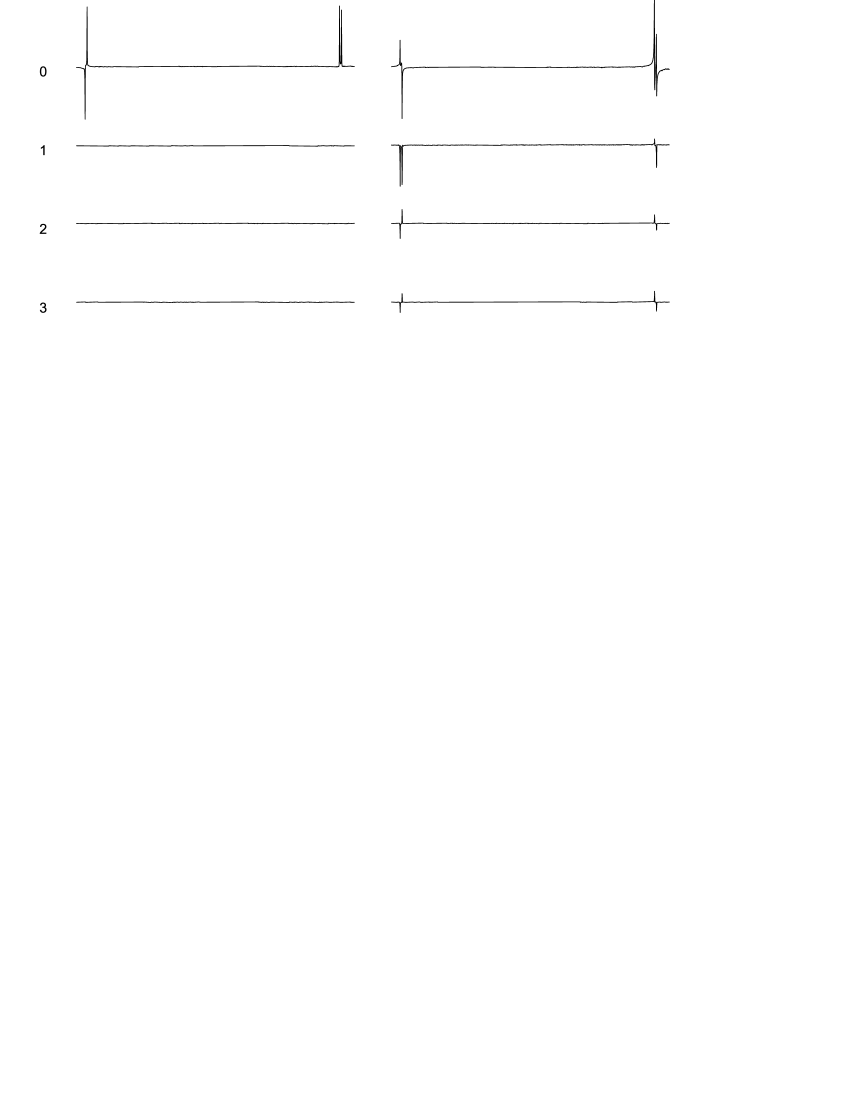
Figure 1: Experimental spectra depicting an implementation of an ensemble twirl. Spectra were obtained using the pulse sequences listed in table 1. The four rows correspond to spectra acquired after 0, 1, 2 or 3 stages of the twirl sequence, while the left and right columns correspond to direct signal acquisition and acquisition after the selective excitation sequence. The ideal result at the end of the full twirl (last row) is no signal with direct detection (left column), and a pair of antiphase doublets with equal and opposite intensities after a selective excitation sequence (right column).

The initial state $\rho$ contains many different components, and the observed spectra (top row) are complicated, reflecting this fact. After the first stage of the twirl sequence (the first field gradient) all components which are directly observable by NMR are crushed (averaged to zero), and so no signal is visible in the direct detection spectrum, but many other components remain, indicated by the variety of signals seen after excitation.

The second stage of the twirl (the $90_{x}$ pulse and the second gradient) removes most of these terms, producing a Bell diagonal state with equal populations of $|\Phi^{+}\rangle$ and $|\Phi^{-}\rangle$. As before there is no signal in the left hand spectrum, while the spectrum on the right contains two antiphase doublets with clearly different intensities. This intensity difference arises from the imbalance between the $|\Psi^{+}\rangle$ state and the two $|\Phi^{\pm}\rangle$ states anwar03 .

After the third and final stage of the twirl (the $54.74_{x}$ pulse and the last gradient) these two antiphase doublets have equal and opposite intensities, characteristic of a Werner singlet state. The final intensity of these doublets, compared with a calibration spectrum (not shown) acquired from the thermal state, is consistent with the twirl preserving the fraction of the singlet state as expected.

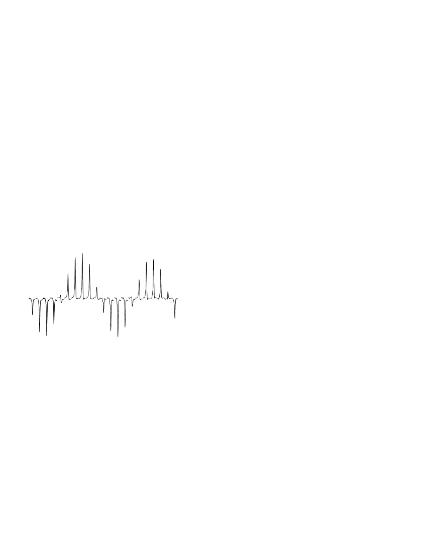
Figure 2: Spectra from Werner singlet states obtained by twirling impure states with varying singlet fractions; only one component of one antiphase doublet is shown. Successive spectra are obtained by incrementing the variable delay in the preparation sequence, Eq. 11, in steps of $1/(10\nu_{I})=\text{\mbox{$218\,\text{$\mu$s}$}}$, which causes the fraction of singlet in the initial state to be modulated, with a period of ten steps.

This last point is explored in more detail in the second experiment, in which the full twirl is applied to a range of initial states with different amounts of the singlet state. The size of the singlet component for our family of states is given in Equation 12, and shows two kinds of sinusoidal modulation with the variable delay $\tau$: a fast variation, arising from the offset frequency $\nu_{I}$, on top of a slow variation due to the coupling $J$ between the two qubits. If we choose $\tau$ to be close to $1/(2J)$, we are near the maximum of the slow $J$ modulation, and the effect of varying $\tau$ is dominated by a sinusoidal variation arising from $\nu_{I}$.

In this way we can produce a range of density matrices $\rho$ with varying amounts of singlet, together with other terms, each of which can be twirled to produce a Werner state. This state can then be observed using a selective excitation pulse prior to acquisition. In each case the expected spectrum is a pair of antiphase doublets, with the intensity of the signal showing a sinusoidal modulation at the frequency $\nu_{I}$. The results of this experiment are shown in Fig. 2, which depicts the intensity variation in the righthand component of the lefthand doublet as $\tau$ is varied around a value of $1/(2J)=\mbox{$69.3\,\text{ms}$}$, with an increment between successive spectra of $1/(10\nu_{I})=\text{\mbox{$218\,\text{$\mu$s}$}}$; equivalent effects can be seen for the other three components of the NMR signal. As expected a sinusoidal modulation of the signal is clearly seen, and the observed modulation period of ten spectra is exactly as expected. The small out of phase signals observable near the zero-crossings of the sine wave can be ascribed to the effects of spin–lattice relaxation during the gradient pulses.

V Conclusions

We have described a variety of strategies for the practical implementation of twirl sequences on conventional and ensemble quantum computers, and have demonstrated an ensemble implementation on an NMR quantum computer. With a conventional quantum computer the implementation requiring the smallest number of different bilateral operations is the set of 12 rotations previously described bennett96b , but our 18 step and 27 step averaging procedures require a smaller number of elementary operations and may be simpler to implement in practice. With an ensemble quantum computer, such as an NMR device, it can be simpler to replace the discrete averaging procedure by continuous averaging, exploiting the ensemble nature of the system. We have developed a scheme, involving the application of three successive crush gradients separated by RF pulses, which is well suited to NMR quantum computers, and have demonstrated that its experimental performance is consistent with theoretical expectations.

- (1) C. H. Bennett, G. Brassard, S. Popescu, B. Schumacher, J. A. Smolin, and W. K. Wootters, Phys. Rev. Lett. 76, 722 (1996); eprint quant-ph/9511027.
- (2) C. H. Bennett, D. P. DiVincenzo, J. A. Smolin, and W. K. Wootters, Phys. Rev. A 54, 3824 (1996); eprint quant-ph/9604024.
- (3) R. F. Werner, Phys. Rev. A 40, 4277 (1989).
- (4) J. Keeler, R. T. Clowes, A. L. Davis, and E. Laue, Methods Enzymol 239, 145 (1994).
- (5) D. G. Cory, A. F. Fahmy, T. F. Havel, in “PhysComp ’96” (T. Toffoli, M. Biafore and J. Leão, Eds.), pp. 87–91, New England Complex Systems Institute (1996).
- (6) J. A. Jones, Prog. Nucl. Magn. Reson. Spectrosc. 38, 325 (2001).
- (7) J. A. Jones, M. Mosca, and R. H. Hansen, Nature 393, 344 (1998).
- (8) M. A. Nielsen, E. Knill, and R. Laflamme, Nature 396, 52 (1998).
- (9) M. S. Anwar, D. Blazina, H. Carteret, S. B. Duckett, T. K. Halstead, J. A. Jones, C. M. Kozak, and R. J. K. Taylor, Phys. Rev. Lett. 93, 040501 (2004).
- (10) M. A. Nielsen and I. L. Chuang, Quantum Computation and Quantum Information (Cambridge University Press, 2000).
- (11) P. Hayden, D. Leung, P. W. Shor, and A. Winter, eprint quant-ph/0307104.
- (12) K. Schmidt-Rohr, and H. W. Spiess, Multidimensional Solid-State NMR and Polymers (Academic Press, London, 1994).
- (13) H. F. Jones, Groups, Representations and Physics (Institute of Physics Publishing, Bristol and Philadelphia, 1996).
- (14) A. Bax, N. M. Szeverenyi, and G. E. Maciel, J. Magn. Reson. 52, 147 (1983).
- (15) L. Viola, E. Knill, and S. Lloyd, Phys. Rev. Lett. 82, 2417 (1999); eprint quant-ph/9809071.
- (16) L. Viola, J. Mod. Opt. (2004, in press); eprint quant-ph/0404038.
- (17) P. K. Aravind, Phys. Lett. A 233, 7 (1997).
- (18) O. W. Sørensen, G. W. Eich, M. H. Levitt, G. Bodenhausen, and R. R. Ernst, Prog. Nucl. Magn. Reson. Spectrosc. 16, 163 (1983).
- (19) E. M. Fortunato, M. A. Pravia, N. Boulant, G. Teklemariam, T. F. Havel, and D. G. Cory, J. Chem. Phys. 116, 7599 (2002)
- (20) J. A. Jones, and M. Mosca, Phys. Rev. Lett. 83, 1050 (1999).