Abstract

We make a brief review of the Kramers escape rate theory for the probabilistic motion of a particle in a potential well $U(x)$, and under the influence of classical fluctuation forces. The Kramers theory is extended in order to take into account the action of the thermal and zero-point random electromagnetic fields on a charged particle. The result is physically relevant because we get a non null escape rate over the potential barrier at low temperatures ($T\rightarrow 0$). It is found that, even if the mean energy is much smaller than the barrier height, the classical particle can escape from the potential well due to the action of the zero-point fluctuating fields. These stochastic effects can be used to give a classical interpretation to some quantum tunneling phenomena. Relevant experimental data are used to illustrate the theoretical results.

Keywords: Foundations of quantum mechanics; zero-point radiation

1 Introduction

One of the most useful contributions to our understanding of the stochastic processes theory is the study of escape rates over a potential barrier. The theoretical approach, first proposed by Kramers [1], has many applications in chemistry kinetics, diffusion in solids, nucleation [2], and other phenomena [3]. The essential structure of the escape process is that the bounded particle is under the action of three types of forces: a deterministic nonlinear force with at least one metastable region, a fluctuating force whose action is capable of pushing the particle out of the metastable region, and a dissipative force which inevitably accompany the fluctuations.

In this work we describe the escape rates of a particular model: a classical charged particle moving in the metastable potential shown in the Figure 1, and under the influence of the fluctuating electromagnetic radiation forces commonly used in Stochastic Electrodynamics (SED)[4, 5]. The fluctuating fields postulated in SED are classical random fields, with zero mean but nonzero higher moments. The spectral distribution of this radiation can be expressed as a sum of two terms

$$\rho(\omega,T) = \frac{\omega^{2}}{\pi^{2}c^{3}}\left[\frac{\hbar\omega}{2}+\frac{\hbar\omega}{e^{\hbar\omega/k_{B}T}-1}\right]$$ (1)

The first term is the zero-point radiation contribution to the spectral distribution. It is independent of the temperature and is Lorentz invariant. The second term in (1) is the blackbody radiation spectral distribution, responsible for the temperature effects on the system.

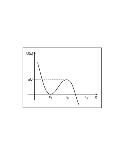
Figure 1: Metastable potential with a barrier height $\Delta U=U(x_{b})-U(x_{a})$, a local minimum $x_{a}$ and a local maximum $x_{b}$ (top of the barrier).

2 Properties of the harmonic oscillator motion under the action of a thermal and zero-point radiation

The zero-point radiation (first term in (1)) has a mean energy $\hbar\omega/2$ associated with each mode of the electromagnetic fields, and is responsible for the most important features of SED. With this zero-point radiation postulated, several phenomena associated with the quantum behavior of the microscopic world can be explained on classical grounds. Many examples can be found in the reviews [5, 6, 7, 8].

The potential $U(x)$ will be approximated by a harmonic oscillator in the region of the potential well $(x\approx x_{a})$ so that (see Figure 1)

$$U(x)\simeq U(x_{a})+\frac{1}{2}m\omega_{a}^{2}(x-x_{a})^{2},$$ (2)

where $\omega_{a}$ is the natural frequency of the oscillator.

The dynamical behavior of a harmonically bounded charged particle has been extensively studied in the context of classical SED. It is found that the zero-point radiation maintains the stability of this system. We shall use the statistical properties of the harmonic oscillator in order to understand, classically, the escape rate at very low temperatures. We give below a brief review of the harmonic motion under the action of the random electric fields characteristic of SED.

The nonrelativistic motion of the charged particle (charge $e$ and mass $m$) near the bottom of the potential well (see Figure 1) is governed by the equation

$$m\ddot{\xi}=-m\omega_{a}^{2}\xi+\frac{2e^{2}}{3c^{3}}\stackrel{{\scriptstyle\ldots}}{{\xi}}+eE_{x}(t),$$ (3)

where $\xi=x-x_{a}$, and $E_{x}(t)$ is the $x$ component of the random electric field. The term proportional to $\stackrel{{\scriptstyle\ldots}}{{\xi}}$ is the radiation reaction force. The electric field is such that $\left\langle E_{x}(t)\right\rangle=0$ and

$$\left\langle E_{x}(t)E_{x}(0)\right\rangle=\frac{4\pi}{3}\int^{\infty}_{0}d\omega\rho(\omega,T)\cos(\omega t),$$ (4)

where the spectral distribution $\rho(\omega,T)$ was introduced in the equation (1). The radiation reaction force can be approximated by [9]

$$\frac{2e^{2}}{3c^{3}}\stackrel{{\scriptstyle\ldots}}{{\xi}}\simeq-m\gamma\dot{\xi},$$ (5)

where $\gamma=2e^{2}\omega_{a}^{2}/3mc^{3}$. Moreover it is verified that $\gamma\ll\omega_{a}$. According to these approximations one can show that the average energy $\langle\epsilon\rangle$ of the oscillating charge is such that

$$\langle\epsilon\rangle=\frac{1}{2}m\langle\dot{\xi}^{2}\rangle+\frac{1}{2}m\omega_{a}^{2}\langle\xi^{2}\rangle=\frac{\hbar\omega_{a}}{2}\coth\left(\frac{\hbar\omega_{a}}{2k_{B}T}\right)\equiv D(T),$$ (6)

where we have introduced the function $D(T)$ in order to simplify our notation. Notice that the average energy depends on the temperature and on the oscillatory frequency $\omega_{a}$.

The result (6) is well known [5]. The average energy $\langle\epsilon\rangle$ becomes equal to $k_{B}T$ in the high temperature limit ($k_{B}T\gg\hbar\omega_{a}$), and is non zero when $T=0$. Actually $D(T)\rightarrow\hbar\omega_{a}/2$ as $T\rightarrow 0$. Notice that $D(T)$ depends on $\hbar$. We can show that the Planck constant comes from the intensity of the zero-point field $E_{x}(t)$ that appears in (3). We recall that $\hbar\omega_{a}/2$ is the value of the ground state energy of the harmonic oscillator in quantum mechanics. This result, obtained within the realm of SED, differs from the usual null result of ordinary classical physics because the zero-point fluctuations are taken into account.

It is quite natural to use the average energy (6) in the calculation of the Kramers escape rate of a potential well. We shall see that the consequence of the new form of the average energy is a non-vanishing escape rate even if $T\rightarrow 0$. Most authors do not mention the classical zero-point fluctuations and use the quantum mechanical formalism to interpret the non null escape rate as a tunneling through the classical forbidden region of the barrier. We shall see that the zero-point fluctuations allow the escape over the potential barrier even if the mean energy of the particle inside the barrier is much less than $\Delta U=U(x_{b})-U(x_{a})$. In the classical mechanics context the escape would be impossible without the action of the zero-point fluctuations. For simplicity we shall take $U(x_{a})=0$ in what follows.

3 The escape rate over the potential well

We shall use the approach of Chandrasekhar [10], based on the Kramers theory. The physical system considered by Chandrasekhar is a particle moving under the influence of a fluctuating force, and a potential $U(x)$ that has a metastable region (see Figure 1). The motion of the particle is governed by a Langevin type equation

$$m\ddot{x}=-m\gamma\dot{x}-U^{\prime}(x)+F(t),$$ (7)

where $-m\gamma\dot{x}$ is the dissipative force and $F(t)$ is the fluctuating force which is characterized by the average $\langle F(t)\rangle=0$. The average energy of the particle within the potential well, that is $x<x_{b}$, is assumed to be given by

$$\langle\frac{m}{2}\dot{x}^{2}+U(x)\rangle=k_{B}T,$$ (8)

in the high temperature limit.

It is possible to show that the Langevin equation (7) leads to a phase space Fokker-Planck equation given by [10]

$$\frac{\partial W}{\partial t}+\frac{p}{m}\frac{\partial W}{\partial x}-U^{\prime}(x)\frac{\partial W}{\partial p}=\gamma W+\gamma p\frac{\partial W}{\partial p}+m\gamma k_{B}T\frac{\partial^{2}W}{\partial p^{2}},$$ (9)

where $W=W(x,p,t)$ is the probability distribution in phase space. Notice that the left hand side of the above expression is equivalent to the Liouville equation. The right hand side appears as a consequence of the fluctuating and dissipation forces. For low temperatures, the Fokker-Planck equation (9) is not valid. As we have mentioned in previous section (see the equation (6)), the factor $k_{B}T$ in the last term of (9) must be replaced by $D(T)=\frac{\hbar\omega_{a}}{2}\coth\left(\frac{\hbar\omega_{a}}{2k_{B}T}\right)$. Therefore, we shall consider the following equation

$$\frac{\partial W}{\partial t}+\frac{p}{m}\frac{\partial W}{\partial x}-U^{\prime}(x)\frac{\partial W}{\partial p}=\gamma W+\gamma p\frac{\partial W}{\partial p}+m\gamma D(T)\frac{\partial^{2}W}{\partial p^{2}}.$$ (10)

We shall see that the equation (10) will allow us to give an accurate description of the escape rate at low temperatures.

In the Kramers theory, two quantities are essential to calculate the escape rate. One is the probability $P(t)$ of finding the particle inside the potential well. This probability can be obtained from the phase space distribution, namely

$$P(t)=\int_{-\infty}^{\infty}dp\int_{-\infty}^{x_{b}}dxW(x,p,t).$$ (11)

The other important quantity is the diffusion current, $j(x_{b})$, across the top of the potential barrier. The diffusion current in an arbitrary position $x$ is defined by

$$j(x,t)\equiv\int_{-\infty}^{\infty}dp\frac{p}{m}W(x,p,t).$$ (12)

Using (10), (11) and (12) one can show that

$$\frac{\partial P(t)}{\partial t}=-\int_{-\infty}^{\infty}dp\frac{p}{m}W(x_{b},p,t)=-j(x_{b},t).$$ (13)

The escape rate $\kappa$, regarded as the decay factor of the probability $P(t)$, can be defined by the equation

$$\frac{\partial P(t)}{\partial t}=-\kappa P(t).$$ (14)

The solution of the above equation is

$$P(t)=P_{0}e^{-\kappa t},$$ (15)

where $P_{0}$ is a constant that will be calculated later. On the other hand, consistently with the equations (13) and (14), one can define the escape rate as

$$\kappa\equiv\frac{j(x_{b},t)}{P(t)}.$$ (16)

Therefore, according to the above theory we have

$$W(x,p,t)=Q(x,p)e^{-\kappa t},$$ (17)

where $Q(x,p)$ satisfies the equation

$$\frac{p}{m}\frac{\partial Q}{\partial x}-U^{\prime}(x)\frac{\partial Q}{\partial p}-\gamma Q-\gamma p\frac{\partial Q}{\partial p}-m\gamma D(T)\frac{\partial^{2}Q}{\partial p^{2}}=0.$$ (18)

A physically interesting case could be

$$Q(x,p)\propto\exp\left[-\frac{p^{2}/2m+U(x)}{D(T)}\right],$$ (19)

however, this standard distribution leads to a situation in which there is no diffusion across the potential barrier at $x_{b}$.

Under the conditions of our problem, the equilibrium distribution (19) cannot be valid for all values of $x$. Hence we shall consider a solution of the equation (18) in the following form

$$Q(x,p)=CF(x,p)\exp\left[-\frac{\frac{p^{2}}{2m}+\frac{1}{2}m\omega_{a}^{2}(x-x_{a})^{2}}{D(T)}\right],$$ (20)

where $F(x,p)$ is an unknown function that will be determined below, and $C$ is a normalization constant. Notice that the above expression is valid for the phase space motion near the bottom of the potential well (see Figure 1). The new form for $Q(x,p)$, introduced in (20), requires a boundary condition on $F(x,p)$ for $x\approx x_{a}$, namely $F(x,p)\simeq 1$. An alternative form for this boundary condition is [10]

$$F(x,p)\rightarrow 1,\,\,\,{\rm for}\,\,\,x\ll x_{b}.$$ (21)

Another physical hypothesis is necessary. The probabilistic motion near the top of the barrier $(x\approx x_{b})$ is also governed by a phase space distribution similar to (20), namely

$$Q(x,p)=CF(x,p)\exp\left[-\frac{\frac{p^{2}}{2m}+U(x_{b})-\frac{1}{2}m\omega_{b}^{2}(x-x_{b})^{2}}{D(T)}\right],$$ (22)

because

$$U(x)\simeq U(x_{b})-\frac{1}{2}m\omega_{b}^{2}(x-x_{b})^{2}.$$ (23)

The use of $D(T)$ in both formulas (20) and (22) is justified because we are assuming that the particle stays a long time in the potential well (see section 2), and crosses the top of the barrier very quickly ($\omega_{b}\gg\omega_{a}$).

Since only a few particles can escape over the potential barrier, another boundary condition must be imposed on $F(x,p)$, that is

$$F(x,p)\rightarrow 0,\,\,\,{\rm for}\,\,\,x\gg x_{b}.$$ (24)

Notice that the boundary conditions (21) and (24) are simple hypothesis that can be justified on physical grounds.

Substituting (22) into (18), we obtain the following differential equation for $F(x,p)$,

$$\frac{p}{m}\frac{\partial F}{\partial x}+m\omega_{b}^{2}(x-x_{b})\frac{\partial F}{\partial p}=-\gamma p\frac{\partial F}{\partial p}+m\gamma D(T)\frac{\partial^{2}F}{\partial p^{2}}.$$ (25)

Following Chandrasekhar we assume that $F(x,p)=F\left(p-\alpha m(x-x_{b})\right)\equiv F(y)$, where $\alpha$ will be obtained below. With the introduction of the variable $y$, we obtain the more simple differential equation

$$-(\alpha-\gamma)y\frac{dF}{dy}=m\gamma D(T)\frac{d^{2}F}{dy^{2}},$$ (26)

provided that the constant $\alpha$ is such that

$$\alpha=\frac{\omega_{b}^{2}}{\alpha-\gamma}.$$ (27)

This equation for the constant $\alpha$ has the solutions

$$\alpha=\frac{\gamma}{2}\pm\sqrt{\frac{\gamma^{2}}{4}+\omega_{b}^{2}}.$$ (28)

The single variable differential equation (26) can be integrated giving

$$F=F_{0}\int^{y}_{-\infty}\exp\left[-\frac{(\alpha-\gamma)y^{\prime\,2}}{2m\gamma D(T)}\right]dy^{\prime},$$ (29)

where $F_{0}$ is a constant. One can see that only the positive root in (28) leads to $\alpha-\gamma$ positive, so that $F(y)$ naturally obeys the boundary conditions (21) and (24). Therefore, one can show that

$$F(x,p)=\sqrt{\frac{\alpha-\gamma}{2\pi m\gamma D(T)}}\int^{y}_{-\infty}\exp\left[-\frac{(\alpha-\gamma)y^{\prime\,2}}{2m\gamma D(T)}\right]dy^{\prime}.$$ (30)

Combining (22) and (30) we get for $Q(x,p)$ the result

$$Q(x,p)=C\sqrt{\frac{\alpha-\gamma}{2\pi m\gamma D(T)}}\times$$ (31)

$$\times\exp\left[-\frac{\frac{p^{2}}{2m}+U(x_{b})-\frac{1}{2}m\omega_{b}^{2}(x-x_{b})^{2}}{D(T)}\right]\int^{y}_{-\infty}\exp\left[-\frac{(\alpha-\gamma)y^{\prime\,2}}{2m\gamma D(T)}\right]dy^{\prime}.$$

The equation (31) is valid only in the neighborhood of $x_{b}$. Inside the potential well ($x\approx x_{a}$) the approximate solution is (see section 2)

$$Q(x,p)=C\exp\left[-\frac{\frac{p^{2}}{2m}+\frac{1}{2}m\omega_{a}^{2}(x-x_{a})^{2}}{D(T)}\right].$$ (32)

Using the expression (32), and considering the equations (11), (15) and (17), we obtain for the constant $P_{0}$

$$P_{0} = \int_{-\infty}^{\infty}dp\int_{-\infty}^{\infty}dxC\exp\left[-\frac{\frac{p^{2}}{2m}+\frac{1}{2}m\omega_{a}^{2}(x-x_{a})^{2}}{D(T)}\right]=$$ (33)

$$= C\frac{2\pi D(T)}{\omega_{a}}.$$

The diffusion current across the top of the barrier is (see (12) and (17))

$$j(x_{b})=\int_{-\infty}^{\infty}dp\frac{p}{m}Q(x=x_{b},p),$$ (34)

where $Q(x=x_{b},p)$ is given by our expression (31). From (34) we get

$$j(x_{b}) = C\sqrt{\frac{a-\gamma}{2\pi m\gamma D(T)}}\exp\left[-\frac{U(x_{b})}{D(T)}\right]\times$$

$$\times \int_{-\infty}^{\infty}dp\frac{p}{m}\exp\left[-\frac{p^{2}}{2mD(T)}\right]\int^{p}_{-\infty}dy^{\prime}\exp\left[-\frac{(\alpha-\gamma)y^{\prime\,2}}{2m\gamma D(T)}\right].$$

It is straightforward to show that

$$j(x_{b})=C\sqrt{\frac{\alpha-\gamma}{\alpha}}D(T)\exp\left[-\frac{U(x_{b})}{D(T)}\right].$$ (36)

The escape rate $\kappa$, defined in (16), becomes

$$\kappa=\frac{j(x_{b})}{P_{0}}=\frac{\omega_{a}}{2\pi}\sqrt{\frac{\alpha-\gamma}{\alpha}}\exp\left[-\frac{U(x_{b})}{D(T)}\right],$$ (37)

independently of the normalization constant $C$. Notice that the exponential factor $e^{-\kappa t}$, present in $j(x_{b},t)$ and $P(t)$, cancels leading to the result (37).

From the expression (28) for the positive root, it is possible to show that

$$\kappa=\frac{\omega_{a}}{2\pi\omega_{b}}\left(\sqrt{\frac{\gamma^{2}}{4}+\omega_{b}^{2}}-\frac{\gamma}{2}\right)\exp\left[-\frac{\Delta U}{D(T)}\right].$$ (38)

Notice that in the low friction limit $\gamma\rightarrow 0$, this expression is the simple formula $\kappa\simeq(\omega_{a}/2\pi)\exp{(-\Delta U/D)}$. It is very important to remark that, in this equation, the escape rate depends on the potential height $\Delta U$, and on the parameters characterizing the particle motion inside the barrier, namely, the frequency $\omega_{a}$ and the average energy $\langle\epsilon\rangle=D(T)=\frac{\hbar\omega_{a}}{2}\coth\left(\frac{\hbar\omega_{a}}{2k_{B}T}\right)$. We recall that $\langle\epsilon\rangle=k_{B}T$ when the temperature is high enough.

4 Comparison with experimental data and conclusion

In order to illustrate, in a quantitative manner, the great analogy between the quantum tunneling description and our classical stochastic escape rate calculation, the experimental results of Alberding et al. [11] will be used. Notice that

$$\frac{\gamma}{\omega_{b}}\ll\frac{\gamma}{\omega_{a}}=\frac{e^{2}}{\hbar c}\frac{\hbar\omega_{a}}{mc^{2}}\ll 1,$$ (39)

so that the expression (38) can be written in the form

$$\kappa(T)=\frac{\omega_{a}}{2\pi}\exp\left(-\frac{\Delta U}{\frac{\hbar\omega_{a}}{2}\coth\left(\frac{\hbar\omega_{a}}{2k_{B}T}\right)}\right).$$ (40)

According to Alberding et al., the beta-chain of hemoglobin ($\beta Hb$) is bounded to the carbon monoxide $CO$ from which it can be separated with a LASER. The rate of recombination can be obtained experimentally. The fraction $N(t)$ of the molecules that have not been recombined with $CO$ is measured as a function of time. Then, the time $\tau$, necessary to reduce $N(t)$ to 75% of its original value, is determined. It is assumed that this recombination is a passage through the potential barrier and a good estimate of the escape rate is $\kappa=1/\tau$.

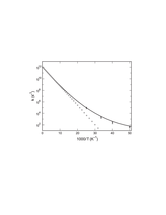
Figure 2: The solid line gives the high temperature behavior of our theoretical prediction (formula (40)). The intermediate temperature experimental data for the escape rate associated to the CO migration to a separated $\beta$ chain of hemoglobin are plotted (Alberding et al., 1976). The open circles corresponds to the escape rate without the zero-point fluctuations, namely the Arrhenius formula $\kappa=\frac{\omega_{a}}{2\pi}\exp(-\Delta U/k_{B}T)$.

This experimental procedure can be repeated for different temperatures $T$. The result for $\kappa(T)$ is indicated by the experimental points (black dots) in the Figures 2 and 3, obtained by N.R. Alberding and collaborators. We shall see that these experimental data are very well described by the formula (40).

We have adjusted the values of $\omega_{a}$ and $\Delta U$ so that the experimental data and the formula (40) are in good agreement. The values obtained are

$$\frac{\hbar\omega_{a}}{2}=2.53\cdot 10^{-3}eV,$$

$$\Delta U=6.68\cdot 10^{-2}eV.$$ (41)

Notice the impressive agreement between the classical theory with zero-point radiation and the experimental data. This is more clearly seen in the Figure 3. We conclude that the particle can escape from the potential well at $T\rightarrow 0$, despite the fact that the barrier height $\Delta U$ is much bigger than the particle mean energy $\hbar\omega_{a}/2$ inside the well ($2\Delta U/\hbar\omega_{a}\approx 26$).

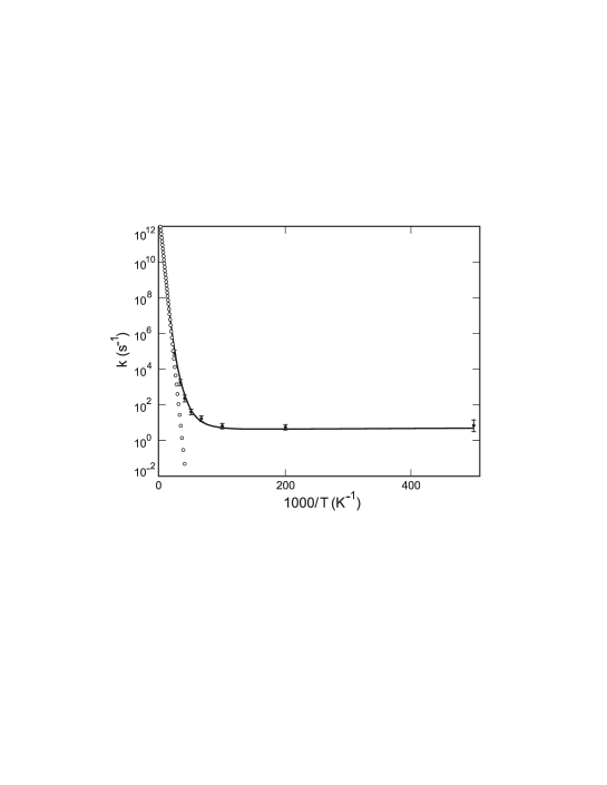
Figure 3: Experimental data for the escape rate associated to the CO migration to a separated $\beta$ chain of hemoglobin (Alberding et al., 1976). The solid line is our theoretical result (see formula (40)). The open circles correspond to the escape rate without the zero-point fluctuations (Arrhenius formula).

It is interesting to recall that Alberding et al. have obtained $\Delta U$ using a conventional quantum mechanics calculation. They have found a value for $\Delta U$ which is in semi-quantitative agreement with the value obtained by us. However, the frequency $\omega_{a}$ was not obtained by Alberding et al.. We want to stress that the frequency $\omega_{a}$ gives relevant information about the potential well (see (2)).

The classical stochastic interpretation of the zero temperature escape rate is that the zero-point fluctuations provide enough energy so that the particle can go over the potential barrier. Since the particle is subjected to both the fluctuation and the dissipation processes associated with the radiation bath, the energy is not a constant of the motion. Therefore, particles that are initially inside the potential well can escape and be detected at points $x_{c}\gg x_{b}$ (see Figure 1), with a fluctuating energy $\epsilon(t)<\Delta U$, contrary to the criticism of Baublitz concerning the SED type calculation [12]. Therefore, the classical escape rate calculation presented in our paper gives results entirely analogous to the quantum tunneling description, provided that the electromagnetic zero-point fluctuations are included in the calculations.

References

- [1] H.A. Kramers, “Brownian motion in a field of force and the diffusion model of chemical reactions”, Physica 7 (1940) 284.
- [2] P. Hänggi, P. Talkner and M. Borkovec, “Reaction-rate theory: fifty years after Kramers”, Rev. Mod. Phys. 62 (1990) 251.
- [3] T.W. Marshall and E. Santos, “Semiclassical treatment of macroscopic quantum relaxation”, Anales de Fisica 91 (1995) 49.
- [4] T.W. Marshall, “Random electrodynamics”, Proc. Royal Soc. London 276A (1963) 475.
- [5] T.H. Boyer, “Random electrodynamics: The theory of classical electrodynamics with classical electromagnetic zero-point radiation”, Phys. Rev. D 11 (1975) 790.
- [6] T.H. Boyer, “A Brief Survey of Stochastic Electrodynamics” in: A.O. Barut, editor, Foundations of Radiation Theory and Quantum Electrodynamics, pg. 49. Plenum Press, New York, 1980.
- [7] L. de la Peña and A.M. Cetto, The Quantum Dice. An Introduction to the Stochastic Electrodynamics. Kluwer Academic, Dordrecht, 1996.
- [8] P.W. Milonni, “Semiclassical and quantum-electrodynamical approaches in nonrelativistic radiation theory”, Phys. Rep. 25 (1976) 1.
- [9] J.D. Jackson, Classical Electrodynamics, 2nd ed. Jonh Wiley & Sons, New York, 1975. Chapters 9 and 17.
- [10] S. Chandrasekhar, “Stochastic Problems in Physics and Astronomy”, Rev. Mod. Phys. 15 (1943) 1.
- [11] N. Alberding, R.H. Austin, K.W. Beeson, S.S. Chan, L. Eisenstein, H. Frauenfelder and T.M. Nordlund, “Tunneling in ligand binding to heme proteins”, Science 192 (1976) 1002.
- [12] M. Baublitz Jr., “Electron field-emission data, quantum mechanics, and the classical stochastic theories”, Phys. Rev. A 51 (1995) 1677.