Is repulsive Casimir force physical?111This paper is based on my Ph.D. dissertation in physics at Virginia Polytechnic Institute and State University, April (2004) key-Sung-Nae-Cho .

Sung Nae Cho sucho2@vt.edu Department of Physics, Virginia Polytechnic Institute and State University, Blacksburg, Virginia 24061, USA
(Monday, August 30, 2004 )
Abstract

The Casimir force for charge-neutral, perfect conductors of non-planar geometric configurations have been investigated. The configurations are: (1) the plate-hemisphere, (2) the hemisphere-hemisphere and (3) the spherical shell. The resulting Casimir forces for these physical arrangements have been found to be attractive. The repulsive Casimir force found by Boyer for a spherical shell is a special case requiring stringent material property of the sphere, as well as the specific boundary conditions for the wave modes inside and outside of the sphere. The necessary criteria in detecting Boyer’s repulsive Casimir force for a sphere are discussed at the end of this investigation.

pacs:
12.20.-m

I Introduction

When two electrically neutral, conducting plates are placed parallel to each other, our understanding from classical electrodynamics tells us that nothing should happen to these plates. The plates are assumed to be that made of perfect conductors for simplicity. In 1948, H. B. G. Casimir and D. Polder faced a similar problem in studying forces between polarizable neutral molecules in colloidal solutions. Colloidal solutions are viscous materials, such as paint, that contain micron-sized particles in a liquid matrix. It had been thought that forces between such polarizable, neutral molecules were governed by the van der Waals interaction. The van der Waals interaction is also referred to as the “Lennard-Jones interaction.” It is a long range electrostatic interaction that acts to attract two nearby polarizable molecules. Casimir and Polder found to their surprise that there existed an attractive force which could not be ascribed to the van der Waals theory. Their experimental result could not be correctly explained unless the retardation effect was included in van der Waals’ theory. This retarded van der Waals interaction or Lienard-Wiechert dipole-dipole interaction is now known as the Casimir-Polder interaction key-Casimir-Polder ; key-Lifshitz ; key-Schwinger-DeRaas-Milton ; key-Milonni ; key-Milton . Casimir, following this first work, elaborated on the Casimir-Polder interaction in predicting the existence of an attractive force between two electrically neutral, parallel plates of perfect conductors separated by a small gap key-Casimir . This alternative derivation of the Casimir force is in terms of the difference between the zero-point energy in vacuum and the zero-point energy in the presence of boundaries. This force has been confirmed by experiments key-Lamoreaux ; key-Mohideen ; key-Bressi-Carugno-Onofrio-Ruoso ; key-Yale-Group-Casimir-Polder and the phenomenon is what is now known as the “Casimir Effect.” The force responsible for the attraction of two uncharged conducting plates is accordingly termed the “Casimir Force.” It was shown later that the Casimir force could be both attractive or repulsive depending on the geometry and the material property of the conductors key-Boyer ; key-Maclay ; key-Kenneth-Klich-Mann-Revzen .

Refer to caption
Figure 1: The vacuum polarization of a photon.

The Casimir effect is regarded as macroscopic manifestation of the retarded van der Waals interaction between uncharged polarizable molecules (or atoms). Microscopically, the Casimir effect is due to interactions between induced multipole moments, where the dipole term is the most dominant contributor if it is non-vanishing. Therefore, the dipole interaction is exclusively referred to, unless otherwise explicitly stated, throughout this investigation. The induced dipole moments can be qualitatively explained by the concept of “vacuum polarization” in quantum electrodynamics (QED). The idea is that a photon, whether real or virtual, has a charged particle content. Namely, the internal loop, illustrated in Figure 1, can be $e^{+}e^{-},$ $\mu^{+}\mu^{-},$ $\tau^{+}\tau^{-},$ $\pi^{+}\pi^{-}$ or $q\bar{q}$ pairs, etc. Its correctness have been born out from the precision measurements of Lamb shift key-Lundeen-Pipkin ; key-Dubler-et-al and photoproduction key-photo-pro-M-Ya-Amusia ; key-photo-pro-F-J-Gilman ; key-photo-pro-Lautrup-Peterman-Rafael ; key-photo-pro-Krawczyk-Zembrzuski-Staszel experiments over a vast range of energies. For the almost zero energy photons considered in the Casimir effect, these pairs last for a time interval $\triangle t$ consistent with that given by the Heisenberg uncertainty principle $\triangle E\cdot\triangle t=h,$ where $\triangle E$ is the energy imbalance and $h$ is the Planck constant. These virtual charged particles can induce the requisite polarizability on the boundary of the dielectric (or conducting) plates which explained the Casimir effect. However, the dipole strength is left as a free parameter in the calculations because it cannot be readily calculated key-Uehling . Its value can be determined from experiments.

Once this idea is taken for granted, one can then move forward to calculate the effective, temperature averaged, energy due to the dipole-dipole interactions with the time retardation effect folded in. The energy between the dielectric (or conducting) media is obtained from the allowed modes of electromagnetic waves determined by the Maxwell equations together with the boundary conditions. The Casimir force is then obtained by taking the negative gradient of the energy in space. This approach, as opposed to full atomistic treatment of the dielectrics (or conductors), is justified as long as the most significant photon wavelengths determining the interaction are large when compared with the spacing of the lattice points in the media. The effect of all the multiple dipole scattering by atoms in the dielectric (or conducting) media simply enforces the macroscopic reflection laws of electromagnetic waves. For instance, in the case of the two parallel plates, the most significant wavelengths are those of the order of the plate gap distance. When this wavelength is large compared with the interatomic distances, the macroscopic electromagnetic theory can be used with impunity. The geometric configuration can introduce significant complications, which is the subject matter this study is going to address.

In order to handle the dipole-dipole interaction Hamiltonian in this case, the classical electromagnetic fields have to be quantized into the photon representation first. The photon with non-zero occupation number have energies in units of $\hbar\omega;$ where $\hbar$ is the Planck constant divided by $2\pi,$ and $\omega,$ the angular frequency. The lowest energy state of the electromagnetic fields has energy $\hbar\omega/2.$ They are called the vacuum or the zero point energy state, and they play a major role in the Casimir effect. Throughout this investigation, the terminology “photon” is used to represent the entity with energy $\hbar\omega,$ or the entity with energy $\hbar\omega/2$ unless explicitly stated otherwise. With this in mind, the quantized field energy is written as

$\displaystyle\mathcal{H}^{\prime}_{n_{s},b}$ $\displaystyle=\left[n_{s}+\frac{1}{2}\right]\hbar c\Theta_{k^{\prime}}$
$\displaystyle\times\sum_{n_{1}=0}^{\infty}\sum_{n_{2}=0}^{\infty}\sum_{n_{3}=0}^{\infty}\sqrt{\sum_{i=1}^{3}\left[k^{\prime}_{i}\left(n_{i},L_{i}\right)\right]^{2}},$ (1)

where $c$ is the speed of light in empty space, $\Theta_{k^{\prime}}$ is the degree of freedom in polarization, $k^{\prime}_{i}$ is the wave number, $n_{i}$ is the wave mode number and $L_{i},$ the boundary length. The subscript $b$ of $\mathcal{H}^{\prime}_{n_{s},b}$ denotes the bounded space. For electromagnetic waves, the degree of freedom in polarization, $\Theta_{k^{\prime}}\equiv 2.$ Similarly, in free space, the field energy is quantized in the form

$\displaystyle\mathcal{H}^{\prime}_{n_{s},u}\equiv\mathcal{H}^{\prime}_{n_{s}}$ $\displaystyle=\frac{\left[n_{s}+\frac{1}{2}\right]\hbar c\Theta_{k^{\prime}}}{f_{1}\left(L_{1}\right)f_{2}\left(L_{2}\right)f_{3}\left(L_{3}\right)}\int_{0}^{\infty}\int_{0}^{\infty}$
$\displaystyle\times\int_{0}^{\infty}\sqrt{\sum_{i=1}^{3}\left[k^{\prime}_{i}\left(n_{i},L_{i}\right)\right]^{2}}dk^{\prime}_{1}dk^{\prime}_{2}dk^{\prime}_{3},$ (2)

where the subscript $u$ of $\mathcal{H}^{\prime}_{n_{s},u}$ denotes free (unbounded) space and the functional $f_{i}\left(L_{i}\right)$ in the denominator is equal to $\zeta_{zero}n_{i}^{-1}L_{i}^{-1}$ for a given $L_{i}.$ Here $\zeta_{zero}$ is the zeroes of the function representing the transversal component of the electric field. The corresponding zero point energy for bounded (or unbounded) space is obtained by setting $n_{s}=0$ in equations (1) and (2), respectively.

II Reflection Dynamics

In principle, the atomistic approach utilizing the Casimir-Polder interaction key-Casimir-Polder explains the Casimir effect observed in any system. Unfortunately, the pairwise summation of the intermolecular forces for systems containing large number of atoms can become very complicated. H. B. G. Casimir, realizing the linear relationship between the field and the polarization, devised an easier approach to the calculation of Casimir effect for large systems such as two perfectly conducting parallel plates key-Casimir . The Casimir effect have been also explained by Schwinger utilizing his original invention, “Source Theory” key-Milton ; key-Schwinger-DeRaas-Milton .

In this investigation, we do not follow Casimir’s energy method, nor do we take the route of Schwinger’s source theory. Instead, we adopt the vacuum pressure approach introduced by Milonni, Cook and Goggin key-Milonni-Cook-Goggin , which is a simple elaboration on Casimir’s original calculation technique utilizing the boundary conditions. We choose to consider the vacuum pressure approach over both Casimir’s energy method and Schwinger’s source theory not because it is a superior technique, but simply because it is the easiest one for the physical arrangements considered in this investigation.

The three physical arrangements for the boundary configurations considered in this investigation are: (1) the plate-hemisphere, (2) the hemisphere-hemisphere and (3) a sphere formed by brining two hemispheres together. Because the geometric configurations of items (2) and (3) are special versions of the more general, plate-hemisphere configuration, the basic reflection dynamics needed for the plate-hemisphere case is worked out first. The results can then be applied to the hemisphere-hemisphere and the sphere configurations later.

Refer to caption
Figure 2: The plane of incidence view of plate-hemisphere configuration. The waves that are allowed through internal reflections in the hemisphere cavity must satisfy the relation $\lambda\leq 2\left\|\vec{R^{\prime}}_{2}-\vec{R^{\prime}}_{1}\right\|.$

The vacuum-fields are subject to the appropriate boundary conditions. For boundaries made of perfect conductors, the transverse components of the electric field are zero at the surface. For this simplification, the skin depth of penetration is considered to be zero. The plate-hemisphere under consideration is shown in Figure 2. The solutions to the vacuum-fields are that of the Cartesian version of the free Maxwell field vector potential differential equation $\nabla^{2}\vec{A}\left(\vec{R}\right)-c^{-2}\partial_{t}^{2}\vec{A}\left(\vec{R}\right)=0,$ where the Coulomb gauge $\vec{\nabla}\cdot\vec{A}=0$ and the absence of the source $\rho$ for scalar potential $\Phi$ have been imposed, $\Phi\left(\rho,\left\|\vec{R}\right\|\right)=0.$ The electric and the magnetic field component of the vacuum-field are given by $\vec{E}=-c^{-1}\partial_{t}\vec{A}$ and $\vec{B}=\vec{\nabla}\times\vec{A},$ where $\vec{A}$ is the free field vector potential. The vanishing of the transversal component of the electric field at the perfect conductor surface implies that the solution for $\vec{E}$ is in the form of $\vec{E}\propto\sin\left(2\pi\lambda^{-1}\left\|\vec{L}\right\|\right),$ where $\lambda$ is the wavelength and $\left\|\vec{L}\right\|$ is the path length between the boundaries. The wavelength is restricted by the condition $\lambda\leq 2\left\|\vec{R^{\prime}}_{2}-\vec{R^{\prime}}_{1}\right\|\equiv 2\xi_{2},$ where $\vec{R^{\prime}}_{2}$ and $\vec{R^{\prime}}_{1}$ are two immediate reflection points in the hemisphere cavity of Figure 2. In order to compute the modes allowed inside the hemisphere resonator, a detailed knowledge of the reflections occurring in the hemisphere cavity is needed. This is described in the following section.

II.1 Reflection Points on the Surface of a Resonator

The wave vector directed along an arbitrary direction in Cartesian coordinates is written as

$\displaystyle\vec{k^{\prime}}_{1}\left(k^{\prime}_{1,x},k^{\prime}_{1,y},k^{\prime}_{1,z}\right)$ $\displaystyle=\sum_{i=1}^{3}k^{\prime}_{1,i}\hat{e_{i}},$ (3)

where

$\displaystyle k^{\prime}_{1,i}$ $\displaystyle=\left\{\begin{array}[]{cc}i=1\rightarrow k^{\prime}_{1,x},&\hat{e_{1}}=\hat{x},\\ \\ i=2\rightarrow k^{\prime}_{1,y},&\hat{e_{2}}=\hat{y},\\ \\ i=3\rightarrow k^{\prime}_{1,z},&\hat{e_{3}}=\hat{z}.\end{array}\right.$

Hence, the unit wave vector, $\hat{k^{\prime}}_{1}=\left\|\vec{k^{\prime}}_{1}\right\|^{-1}\sum_{i=1}^{3}k^{\prime}_{1,i}\hat{e_{i}}.$ Define the initial position $\vec{R^{\prime}}_{0}$ for the incident wave $\vec{k^{\prime}}_{1},$

$\displaystyle\vec{R^{\prime}}_{0}\left(r^{\prime}_{0,x},r^{\prime}_{0,y},r^{\prime}_{0,z}\right)$ $\displaystyle=\sum_{i=1}^{3}r^{\prime}_{0,i}\hat{e_{i}},$ (4)

where

$$r^{\prime}_{0,i}=\left\{\begin{array}[]{c}i=1\rightarrow r^{\prime}_{0,x},\\ \\ i=2\rightarrow r^{\prime}_{0,y},\\ \\ i=3\rightarrow r^{\prime}_{0,z}.\end{array}\right.$$

Here it should be noted that $\vec{R^{\prime}}_{0}$ really has only components $r^{\prime}_{0,x}$ and $r^{\prime}_{0,z}.$ But nevertheless, one can always set $r^{\prime}_{0,y}=0$ whenever needed. Since no particular wave vectors with specified wave lengths are prescribed initially, it is desirable to employ a parameterization scheme to represent these wave vectors. The line segment traced out by this wave vector $\hat{k^{\prime}}_{1}$ is formulated in the parametric form

$\displaystyle\vec{R^{\prime}}_{1}$ $\displaystyle=\xi_{1}\hat{k^{\prime}}_{1}+\vec{R^{\prime}}_{0}$
$\displaystyle=\sum_{i=1}^{3}\left[r^{\prime}_{0,i}+\xi_{1}\left\|\vec{k^{\prime}}_{1}\right\|^{-1}k^{\prime}_{1,i}\right]\hat{e_{i}},$ (5)

where the variable $\xi_{1}$ is a positive definite parameter. Here $\vec{R^{\prime}}_{1}$ is the first reflection point on the hemisphere. In terms of spherical coordinate variables, $\vec{R^{\prime}}_{1}$ takes the form

$\displaystyle\vec{R^{\prime}}_{1}\left(r^{\prime}_{i},\theta^{\prime}_{1},\phi^{\prime}_{1}\right)$ $\displaystyle=r^{\prime}_{i}\sum_{i=1}^{3}\Lambda^{\prime}_{1,i}\hat{e_{i}},$ (6)

where

$$\left\{\begin{array}[]{c}\Lambda^{\prime}_{1,1}=\sin\theta^{\prime}_{1}\cos\phi^{\prime}_{1},\\ \\ \Lambda^{\prime}_{1,2}=\sin\theta^{\prime}_{1}\sin\phi^{\prime}_{1},\\ \\ \Lambda^{\prime}_{1,3}=\cos\theta^{\prime}_{1}.\end{array}\right.$$

Here $r^{\prime}_{i}$ is the hemisphere radius, $\theta^{\prime}_{1}$ and $\phi^{\prime}_{1}$ are the polar and the azimuthal angle respectively of $\vec{R^{\prime}}_{1}$ at the first reflection point. Notice that subscript $i$ of $r^{\prime}_{i}$ denotes “inner radius” not a summation index.

By combining equations (5) and (6), we can solve for the parameter $\xi_{1}.$ It can be shown that

$\displaystyle\xi_{1}$ $\displaystyle\equiv\xi_{1,p}$
$\displaystyle=-\hat{k^{\prime}}_{1}\cdot\vec{R^{\prime}}_{0}+\sqrt{\left[\hat{k^{\prime}}_{1}\cdot\vec{R^{\prime}}_{0}\right]^{2}+\left[r^{\prime}_{i}\right]^{2}-\left\|\vec{R^{\prime}}_{0}\right\|^{2}},$ (7)

where the positive root for $\xi_{1}$ have been chosen due to the restriction $\xi_{1}\geq 0.$ The detailed proof of equation (7) is given in Appendix A of reference key-Sung-Nae-Cho . Substituting $\xi_{1}$ in equation (5), the first reflection point off the inner hemisphere surface is expressed as

$\displaystyle\vec{R^{\prime}}_{1}\left(\xi_{1,p};\vec{R^{\prime}}_{0},\hat{k^{\prime}}_{1}\right)$ $\displaystyle=\sum_{i=1}^{3}\left[r^{\prime}_{0,i}+\xi_{1,p}\left\|\vec{k^{\prime}}_{1}\right\|^{-1}k^{\prime}_{1,i}\right]\hat{e_{i}},$ (8)

where $\xi_{1,p}$ is from equation (7).

The incoming wave vector $\vec{k^{\prime}}_{i}$ can always be decomposed into parallel and perpendicular components, $\vec{k^{\prime}}_{i,\parallel}$ and $\vec{k^{\prime}}_{i,\perp},$ with respect to the local reflection surface. It is shown in Appendix A of reference key-Sung-Nae-Cho that the reflected wave vector $\vec{k^{\prime}}_{r}$ has the form

$\displaystyle\vec{k^{\prime}}_{r}$ $\displaystyle=\alpha_{r,\perp}\left[\hat{n^{\prime}}\times\vec{k^{\prime}}_{i}\right]\times\hat{n^{\prime}}-\alpha_{r,\parallel}\hat{n^{\prime}}\cdot\vec{k^{\prime}}_{i}\hat{n^{\prime}},$

where the quantities $\alpha_{r,\parallel}$ and $\alpha_{r,\perp}$ are the reflection coefficients and $\hat{n^{\prime}}$ is a unit surface normal. For the perfect reflecting surfaces, $\alpha_{r,\parallel}=\alpha_{r,\perp}=1.$ In component form,

$\displaystyle\vec{k^{\prime}}_{r}$ $\displaystyle=\sum_{l=1}^{3}\left\{\alpha_{r,\perp}\left[n^{\prime}_{n}k^{\prime}_{i,l}n^{\prime}_{n}-n^{\prime}_{l}k^{\prime}_{i,n}n^{\prime}_{n}\right]\right.$
$\displaystyle\left.-\alpha_{r,\parallel}n^{\prime}_{n}k^{\prime}_{i,n}n^{\prime}_{l}\right\}\hat{e_{l}},$

where it is understood that $\hat{n^{\prime}}$ is already normalized and Einstein summation convention is applied to the index $n.$ The second reflection point $\vec{R^{\prime}}_{2}$ is found then by repeating the steps done for $\vec{R^{\prime}}_{1}$ and by using the expression $\vec{k^{\prime}}_{r}\equiv\vec{k^{\prime}}_{r}/\left\|\vec{k^{\prime}}_{r}\right\|,$

$\displaystyle\vec{R^{\prime}}_{2}$ $\displaystyle=\vec{R^{\prime}}_{1}+\xi_{2,p}\hat{k^{\prime}}_{r}$
$\displaystyle=\vec{R^{\prime}}_{1}+\xi_{2,p}\frac{\alpha_{r,\perp}\left[\hat{n^{\prime}}\times\vec{k^{\prime}}_{i}\right]\times\hat{n^{\prime}}-\alpha_{r,\parallel}\hat{n^{\prime}}\cdot\vec{k^{\prime}}_{i}\hat{n^{\prime}}}{\left\|\alpha_{r,\perp}\left[\hat{n^{\prime}}\times\vec{k^{\prime}}_{i}\right]\times\hat{n^{\prime}}-\alpha_{r,\parallel}\hat{n^{\prime}}\cdot\vec{k^{\prime}}_{i}\hat{n^{\prime}}\right\|},$

where $\xi_{2,p}$ is the new positive definite parameter for the second reflection point.

The incidence plane of reflection is determined solely by the incident wave $\vec{k^{\prime}}_{i}$ and the local normal $\vec{n^{\prime}}_{i}$ of the reflecting surface. It is important to recognize the fact that the subsequent successive reflections of this incoming wave will be confined to this particular incidence plane. This incident plane can be characterized by a unit normal vector. For the system shown in Figure 2,

$\displaystyle\vec{k^{\prime}}_{i}$ $\displaystyle=\vec{k^{\prime}}_{1},$

and

$\displaystyle\vec{n^{\prime}}_{n^{\prime}_{i},1}$ $\displaystyle=-\xi_{1,p}\hat{k^{\prime}}_{1}-\vec{R^{\prime}}_{0}.$

The unit vector which represents the incidence plane is given by

$\displaystyle\hat{n^{\prime}}_{p,1}$ $\displaystyle=-\left\|\vec{n^{\prime}}_{p,1}\right\|^{-1}\sum_{i=1}^{3}\epsilon_{ijk}k^{\prime}_{1,j}r^{\prime}_{0,k}\hat{e_{i}},$

where the summations over indices $j$ and $k$ are implicit. If the plane of incidence is represented by a scalar function $f\left(x^{\prime},y^{\prime},z^{\prime}\right),$ then its unit normal vector $\hat{n^{\prime}}_{p,1}$ will satisfy the relationship $\hat{n^{\prime}}_{p,1}\propto\vec{\nabla^{\prime}}f_{p,1}\left(x^{\prime},y^{\prime},z^{\prime}\right).$ It can be shown (see Appendix A of reference key-Sung-Nae-Cho ) that

$\displaystyle f_{p,1}\left(\nu^{\prime}_{1},\nu^{\prime}_{2},\nu^{\prime}_{3}\right)$ $\displaystyle=-\left\|\vec{n^{\prime}}_{p,1}\right\|^{-1}\sum_{i=1}^{3}\epsilon_{ijk}k^{\prime}_{1,j}r^{\prime}_{0,k}\nu^{\prime}_{i},$ (9)

where

$$i=\left\{\begin{array}[]{c}1\rightarrow\nu^{\prime}_{1}=x^{\prime},\\ \\ 2\rightarrow\nu^{\prime}_{2}=y^{\prime},\\ \\ 3\rightarrow\nu^{\prime}_{3}=z^{\prime}\end{array}\right.$$

and

$$-\infty\leq\left\{\nu^{\prime}_{1}=x^{\prime},\nu^{\prime}_{2}=y^{\prime},\nu^{\prime}_{3}=z^{\prime}\right\}\leq\infty.$$
Refer to caption
Figure 3: The thick line shown here represents the intersection between hemisphere surface and the plane of incidence. The unit vector normal to the plane of incidence is given by $\hat{n^{\prime}}_{p,1}=-\left\|\vec{n^{\prime}}_{p,1}\right\|^{-1}\sum_{i=1}^{3}\epsilon_{ijk}k^{\prime}_{1,j}r^{\prime}_{0,k}\hat{e_{i}}.$

The surface of a sphere or hemisphere is defined through the relation

$\displaystyle f_{hemi}\left(x^{\prime},y^{\prime},z^{\prime}\right)$ $\displaystyle=\left[r^{\prime}_{i}\right]^{2}-\sum_{i=1}^{3}\left[\nu^{\prime}_{i}\right]^{2},$

where $r^{\prime}_{i}$ is the radius of sphere and the subscript $i$ denotes the inner surface. The intercept of interest is shown in Figure 3. The intersection between the hemisphere surface and the incidence plane $f_{p,1}\left(\nu^{\prime}_{1},\nu^{\prime}_{2},\nu^{\prime}_{3}\right)$ is given through the relation

$\displaystyle f_{hemi}\left(x^{\prime},y^{\prime},z^{\prime}\right)-f_{p,1}\left(x^{\prime},y^{\prime},z^{\prime}\right)$ $\displaystyle=0.$

After substitution of $f_{p,1}\left(x^{\prime},y^{\prime},z^{\prime}\right)$ and $f_{hemi}\left(x^{\prime},y^{\prime},z^{\prime}\right),$ we have

$\displaystyle\sum_{i=1}^{3}\left\{\left[\nu^{\prime}_{i}\right]^{2}-\left\|\vec{n^{\prime}}_{p,1}\right\|^{-1}\epsilon_{ijk}k^{\prime}_{1,j}r^{\prime}_{0,k}\nu^{\prime}_{i}\right\}-\left[r^{\prime}_{i}\right]^{2}$ $\displaystyle=0,$

where

$$i=\left\{\begin{array}[]{c}1\rightarrow\nu^{\prime}_{1}=x^{\prime},\\ \\ 2\rightarrow\nu^{\prime}_{2}=y^{\prime},\\ \\ 3\rightarrow\nu^{\prime}_{3}=z^{\prime}.\end{array}\right.$$

The term $\left[r^{\prime}_{i}\right]^{2}$ can be rewritten in the form

$\displaystyle\left[r^{\prime}_{i}\right]^{2}$ $\displaystyle=\sum_{i=1}^{3}\left[r^{\prime}_{i,i}\right]^{2},$

where

$$\left\{\begin{array}[]{c}r^{\prime}_{i,1}=r^{\prime}_{i,x^{\prime}},\\ \\ r^{\prime}_{i,2}=r^{\prime}_{i,y^{\prime}},\\ \\ r^{\prime}_{i,3}=r^{\prime}_{i,z^{\prime}}.\end{array}\right.$$

Solving for $\nu^{\prime}_{i},$ it can be shown (see Appendix A of reference key-Sung-Nae-Cho ) that

$\displaystyle\nu^{\prime}_{i}$ $\displaystyle=\frac{1}{2}\left\|\vec{n^{\prime}}_{p,1}\right\|^{-1}\epsilon_{ijk}k^{\prime}_{1,j}r^{\prime}_{0,k}$
$\displaystyle\pm\sqrt{\left[\frac{1}{2}\left\|\vec{n^{\prime}}_{p,1}\right\|^{-1}\epsilon_{ijk}k^{\prime}_{1,j}r^{\prime}_{0,k}\right]^{2}+\left[r^{\prime}_{i,i}\right]^{2}},$ (10)

where $i=1,2,3$ and $\epsilon_{ijk}$ is the Levi-Civita symbol. The result for $\nu^{\prime}_{i}$ shown above provide a set of discrete reflection points found by the intercept between the hemisphere and the plane of incidence. Using spherical coordinate representations for the variables $r^{\prime}_{i,1},$ $r^{\prime}_{i,2}$ and $r^{\prime}_{i,3},$

$$\left\{\begin{array}[]{c}r^{\prime}_{i,1}=r^{\prime}_{i}\sin\theta^{\prime}\cos\phi^{\prime},\\ \\ r^{\prime}_{i,2}=r^{\prime}_{i}\sin\theta^{\prime}\sin\phi^{\prime},\\ \\ r^{\prime}_{i,3}=r^{\prime}_{i}\cos\theta^{\prime},\end{array}\right.$$

the initial reflection point $\vec{R^{\prime}}_{1}$ can be expressed in terms of the spherical coordinate variables $\left(r^{\prime}_{i},\theta^{\prime}_{1},\phi^{\prime}_{1}\right),$

$\displaystyle\vec{R^{\prime}}_{1}\left(r^{\prime}_{i},\theta^{\prime}_{1},\phi^{\prime}_{1}\right)$ $\displaystyle=\sum_{i=1}^{3}\nu^{\prime}_{1,i}\left(r^{\prime}_{i},\theta^{\prime}_{1},\phi^{\prime}_{1}\right)\hat{e_{i}},$ (11)

where

$$i=\left\{\begin{array}[]{c}1\rightarrow\nu^{\prime}_{1,1}=r^{\prime}_{i}\sin\theta^{\prime}_{1}\cos\phi^{\prime}_{1},\\ \\ 2\rightarrow\nu^{\prime}_{1,2}=r^{\prime}_{i}\sin\theta^{\prime}_{1}\sin\phi^{\prime}_{1},\\ \\ 3\rightarrow\nu^{\prime}_{1,3}=r^{\prime}_{i}\cos\theta^{\prime}_{1}.\end{array}\right.$$

Here $r^{\prime}_{i}$ is the hemisphere radius, $\phi^{\prime}_{1}$ and $\theta^{\prime}_{1},$ the polar and azimuthal angle, respectively. The angles $\phi^{\prime}_{1}$ and $\theta^{\prime}_{1}$ are found to be (see Appendix A of reference key-Sung-Nae-Cho ):

$$\left\{\begin{array}[]{c}\lim_{\varepsilon\rightarrow 0}\left(0\leq\phi^{\prime}_{1}\leq\frac{1}{2}\pi-\left|\varepsilon\right|\right),\\ \\ \lim_{\varepsilon\rightarrow 0}\left(\pi+\left|\varepsilon\right|\leq\phi^{\prime}_{1}\leq\frac{3}{2}\pi-\left|\varepsilon\right|\right),\\ \\ \phi^{\prime}_{1}=\arctan\left(\sqrt{\frac{\Upsilon_{1,2}^{2}-\Upsilon_{1,2}\left\|\vec{n^{\prime}}_{p,1}\right\|^{-1}\epsilon_{2mn}k^{\prime}_{1,m}r^{\prime}_{0,n}}{\Upsilon_{1,1}^{2}-\Upsilon_{1,1}\left\|\vec{n^{\prime}}_{p,1}\right\|^{-1}\epsilon_{1jk}k^{\prime}_{1,j}r^{\prime}_{0,k}}}\right);\end{array}\right.$$ (12)
$$\left\{\begin{array}[]{c}\lim_{\varepsilon\rightarrow 0}\left(\frac{1}{2}\pi+\left|\varepsilon\right|\leq\phi^{\prime}_{1}\leq\pi-\varepsilon\right),\\ \\ \lim_{\varepsilon\rightarrow 0}\left(\frac{3}{2}\pi+\left|\varepsilon\right|\leq\phi^{\prime}_{1}<2\pi-\left|\varepsilon\right|\right),\\ \\ \phi^{\prime}_{1}=\arctan\left(-\sqrt{\frac{\Upsilon_{1,2}^{2}-\Upsilon_{1,2}\left\|\vec{n^{\prime}}_{p,1}\right\|^{-1}\epsilon_{2mn}k^{\prime}_{1,m}r^{\prime}_{0,n}}{\Upsilon_{1,1}^{2}-\Upsilon_{1,1}\left\|\vec{n^{\prime}}_{p,1}\right\|^{-1}\epsilon_{1jk}k^{\prime}_{1,j}r^{\prime}_{0,k}}}\right);\end{array}\right.$$ (13)
$$\left\{\begin{array}[]{c}\lim_{\varepsilon\rightarrow 0}\left(0\leq\theta^{\prime}_{1}\leq\frac{1}{2}\pi-\left|\varepsilon\right|\right),\\ \\ \theta^{\prime}_{1}=\arctan\left(\left[\frac{\Upsilon_{1,1}^{2}+\Upsilon_{1,2}^{2}}{\Upsilon_{1,3}^{2}-\Upsilon_{1,3}\left\|\vec{n^{\prime}}_{p,1}\right\|^{-1}\epsilon_{3qr}k^{\prime}_{1,q}r^{\prime}_{0,r}}\right.\right.\\ \left.\left.-\frac{\Upsilon_{1,1}\epsilon_{1jk}k^{\prime}_{1,j}r^{\prime}_{0,k}+\Upsilon_{1,2}\epsilon_{2mn}k^{\prime}_{1,m}r^{\prime}_{0,n}}{\left\|\vec{n^{\prime}}_{p,1}\right\|\left\{\Upsilon_{1,3}^{2}-\Upsilon_{1,3}\left\|\vec{n^{\prime}}_{p,1}\right\|^{-1}\epsilon_{3qr}k^{\prime}_{1,q}r^{\prime}_{0,r}\right\}}\right]^{1/2}\right);\end{array}\right.$$ (14)
$$\left\{\begin{array}[]{c}\lim_{\varepsilon\rightarrow 0}\left(\frac{1}{2}\pi+\left|\varepsilon\right|\leq\theta^{\prime}_{1}\leq\pi\right),\\ \\ \theta^{\prime}_{1}=\arctan\left(-\left[\frac{\Upsilon_{1,1}^{2}+\Upsilon_{1,2}^{2}}{\Upsilon_{1,3}^{2}-\Upsilon_{1,3}\left\|\vec{n^{\prime}}_{p,1}\right\|^{-1}\epsilon_{3qr}k^{\prime}_{1,q}r^{\prime}_{0,r}}\right.\right.\\ \left.\left.-\frac{\Upsilon_{1,1}\epsilon_{1jk}k^{\prime}_{1,j}r^{\prime}_{0,k}+\Upsilon_{1,2}\epsilon_{2mn}k^{\prime}_{1,m}r^{\prime}_{0,n}}{\left\|\vec{n^{\prime}}_{p,1}\right\|\left\{\Upsilon_{1,3}^{2}-\Upsilon_{1,3}\left\|\vec{n^{\prime}}_{p,1}\right\|^{-1}\epsilon_{3qr}k^{\prime}_{1,q}r^{\prime}_{0,r}\right\}}\right]^{1/2}\right),\end{array}\right.$$ (15)

where

$\displaystyle\Upsilon_{1,i}=r^{\prime}_{0,i}+\xi_{1,p}\left\|\vec{k^{\prime}}_{1}\right\|^{-1}k^{\prime}_{1,i},$ $\displaystyle i=1,2,3.$

Similarly, the second reflection point on the inner hemisphere surface is given by (see Appendix A of reference key-Sung-Nae-Cho ):

$\displaystyle\vec{R^{\prime}}_{2}\left(r^{\prime}_{i},\theta^{\prime}_{2},\phi^{\prime}_{2}\right)$ $\displaystyle=\sum_{i=1}^{3}\nu^{\prime}_{2,i}\left(r^{\prime}_{i},\theta^{\prime}_{2},\phi^{\prime}_{2}\right)\hat{e_{i}},$ (16)

where

$$i=\left\{\begin{array}[]{c}1\rightarrow\nu^{\prime}_{2,1}=r^{\prime}_{i}\sin\theta^{\prime}_{2}\cos\phi^{\prime}_{2},\\ \\ 2\rightarrow\nu^{\prime}_{2,2}=r^{\prime}_{i}\sin\theta^{\prime}_{2}\sin\phi^{\prime}_{2},\\ \\ 3\rightarrow\nu^{\prime}_{2,3}=r^{\prime}_{i}\cos\theta^{\prime}_{2}.\end{array}\right.$$

Here the spherical angles $\phi^{\prime}_{2}$ and $\theta^{\prime}_{2}$ are found to be (see Appendix A of reference key-Sung-Nae-Cho ):

$$\left\{\begin{array}[]{c}\lim_{\varepsilon\rightarrow 0}\left(0\leq\phi^{\prime}_{2}\leq\frac{1}{2}\pi-\left|\varepsilon\right|\right),\\ \\ \lim_{\varepsilon\rightarrow 0}\left(\pi+\left|\varepsilon\right|\leq\phi^{\prime}_{2}\leq\frac{3}{2}\pi-\left|\varepsilon\right|\right),\\ \\ \phi^{\prime}_{2}=\arctan\left(\left\{\left[\frac{1}{2}\left\|\vec{n^{\prime}}_{p,1}\right\|^{-1}\epsilon_{2mn}k^{\prime}_{1,m}r^{\prime}_{0,n}-\grave{\nu}^{\prime}_{2,2}\right]^{2}\right.\right.\\ \left.-\left[\frac{1}{2}\left\|\vec{n^{\prime}}_{p,1}\right\|^{-1}\epsilon_{2mn}k^{\prime}_{1,m}r^{\prime}_{0,n}\right]^{2}\right\}^{1/2}\\ \times\left\{\left[\frac{1}{2}\left\|\vec{n^{\prime}}_{p,1}\right\|^{-1}\epsilon_{1jk}k^{\prime}_{1,j}r^{\prime}_{0,k}-\grave{\nu}^{\prime}_{2,1}\right]^{2}\right.\\ \left.\left.-\left[\frac{1}{2}\left\|\vec{n^{\prime}}_{p,1}\right\|^{-1}\epsilon_{1jk}k^{\prime}_{1,j}r^{\prime}_{0,k}\right]^{2}\right\}^{-1/2}\right);\end{array}\right.$$ (17)
$$\left\{\begin{array}[]{c}\lim_{\varepsilon\rightarrow 0}\left(\frac{1}{2}\pi+\left|\varepsilon\right|\leq\phi^{\prime}_{2}\leq\pi-\varepsilon\right),\\ \\ \lim_{\varepsilon\rightarrow 0}\left(\frac{3}{2}\pi+\left|\varepsilon\right|\leq\phi^{\prime}_{2}<2\pi-\left|\varepsilon\right|\right),\\ \\ \phi^{\prime}_{2}=\arctan\left(-\left\{\left[\frac{1}{2}\left\|\vec{n^{\prime}}_{p,1}\right\|^{-1}\epsilon_{2mn}k^{\prime}_{1,m}r^{\prime}_{0,n}-\grave{\nu}^{\prime}_{2,2}\right]^{2}\right.\right.\\ \left.-\left[\frac{1}{2}\left\|\vec{n^{\prime}}_{p,1}\right\|^{-1}\epsilon_{2mn}k^{\prime}_{1,m}r^{\prime}_{0,n}\right]^{2}\right\}^{1/2}\\ \times\left\{\left[\frac{1}{2}\left\|\vec{n^{\prime}}_{p,1}\right\|^{-1}\epsilon_{1jk}k^{\prime}_{1,j}r^{\prime}_{0,k}-\grave{\nu}^{\prime}_{2,1}\right]^{2}\right.\\ \left.\left.-\left[\frac{1}{2}\left\|\vec{n^{\prime}}_{p,1}\right\|^{-1}\epsilon_{1jk}k^{\prime}_{1,j}r^{\prime}_{0,k}\right]^{2}\right\}^{-1/2}\right);\end{array}\right.$$ (18)
$$\left\{\begin{array}[]{c}\lim_{\varepsilon\rightarrow 0}\left(0\leq\theta^{\prime}_{2}\leq\frac{1}{2}\pi-\left|\varepsilon\right|\right),\\ \\ \theta^{\prime}_{2}=\arctan\left(\left\{\left[\frac{1}{2}\left\|\vec{n^{\prime}}_{p,1}\right\|^{-1}\epsilon_{1jk}k^{\prime}_{1,j}r^{\prime}_{0,k}-\grave{\nu}^{\prime}_{2,1}\right]^{2}\right.\right.\\ -\left[\frac{1}{2}\left\|\vec{n^{\prime}}_{p,1}\right\|^{-1}\epsilon_{1jk}k^{\prime}_{1,j}r^{\prime}_{0,k}\right]^{2}\\ +\left[\frac{1}{2}\left\|\vec{n^{\prime}}_{p,1}\right\|^{-1}\epsilon_{2mn}k^{\prime}_{1,m}r^{\prime}_{0,n}-\grave{\nu}^{\prime}_{2,2}\right]^{2}\\ \left.-\left[\frac{1}{2}\left\|\vec{n^{\prime}}_{p,1}\right\|^{-1}\epsilon_{2mn}k^{\prime}_{1,m}r^{\prime}_{0,n}\right]^{2}\right\}^{1/2}\\ \times\left\{\left[\frac{1}{2}\left\|\vec{n^{\prime}}_{p,1}\right\|^{-1}\epsilon_{3qr}k^{\prime}_{1,q}r^{\prime}_{0,r}-\grave{\nu}^{\prime}_{2,3}\right]^{2}\right.\\ \left.\left.-\left[\frac{1}{2}\left\|\vec{n^{\prime}}_{p,1}\right\|^{-1}\epsilon_{3qr}k^{\prime}_{1,q}r^{\prime}_{0,r}\right]^{2}\right\}^{-1/2}\right);\end{array}\right.$$ (19)
$$\left\{\begin{array}[]{c}\lim_{\varepsilon\rightarrow 0}\left(\frac{1}{2}\pi+\left|\varepsilon\right|\leq\theta^{\prime}_{2}\leq\pi\right),\\ \\ \theta^{\prime}_{2}=\arctan\left(-\left\{\left[\frac{1}{2}\left\|\vec{n^{\prime}}_{p,1}\right\|^{-1}\epsilon_{1jk}k^{\prime}_{1,j}r^{\prime}_{0,k}-\grave{\nu}^{\prime}_{2,1}\right]^{2}\right.\right.\\ -\left[\frac{1}{2}\left\|\vec{n^{\prime}}_{p,1}\right\|^{-1}\epsilon_{1jk}k^{\prime}_{1,j}r^{\prime}_{0,k}\right]^{2}\\ +\left[\frac{1}{2}\left\|\vec{n^{\prime}}_{p,1}\right\|^{-1}\epsilon_{2mn}k^{\prime}_{1,m}r^{\prime}_{0,n}-\grave{\nu}^{\prime}_{2,2}\right]^{2}\\ \left.-\left[\frac{1}{2}\left\|\vec{n^{\prime}}_{p,1}\right\|^{-1}\epsilon_{2mn}k^{\prime}_{1,m}r^{\prime}_{0,n}\right]^{2}\right\}^{1/2}\\ \times\left\{\left[\frac{1}{2}\left\|\vec{n^{\prime}}_{p,1}\right\|^{-1}\epsilon_{3qr}k^{\prime}_{1,q}r^{\prime}_{0,r}-\grave{\nu}^{\prime}_{2,3}\right]^{2}\right.\\ \left.\left.-\left[\frac{1}{2}\left\|\vec{n^{\prime}}_{p,1}\right\|^{-1}\epsilon_{3qr}k^{\prime}_{1,q}r^{\prime}_{0,r}\right]^{2}\right\}^{-1/2}\right),\end{array}\right.$$ (20)

where the variables have the definition:

$$\left\{\begin{array}[]{c}\nu^{\prime}_{1,1}=x^{\prime}_{1}=r^{\prime}_{i}\sin\theta^{\prime}_{1}\cos\phi^{\prime}_{1},\\ \\ \nu^{\prime}_{1,2}=y^{\prime}_{1}=r^{\prime}_{i}\sin\theta^{\prime}_{1}\sin\phi^{\prime}_{1},\\ \\ \nu^{\prime}_{1,3}=z^{\prime}_{1}=r^{\prime}_{i}\cos\theta^{\prime}_{1};\end{array}\right.$$
$\displaystyle\theta_{inc}$ $\displaystyle=\arccos\left(\left\{\sin\theta^{\prime}_{1}\left[k^{\prime}_{x^{\prime}_{1}}\cos\phi^{\prime}_{1}+k^{\prime}_{y^{\prime}_{1}}\sin\phi^{\prime}_{1}\right]\right.\right.$
$\displaystyle\left.\left.+k^{\prime}_{z^{\prime}_{1}}\cos\theta^{\prime}_{1}\right\}\left\{\left[k^{\prime}_{x^{\prime}_{1}}\right]^{2}+\left[k^{\prime}_{y^{\prime}_{1}}\right]^{2}+\left[k^{\prime}_{z^{\prime}_{1}}\right]^{2}\right\}^{-1/2}\right),$ (21)

where $k^{\prime}_{1,1}=k^{\prime}_{x^{\prime}_{1}},$ $k^{\prime}_{1,2}=k^{\prime}_{y^{\prime}_{1}}$ and $k^{\prime}_{1,3}=k^{\prime}_{z^{\prime}_{1}};$ and

$\displaystyle\Gamma_{1,2}$ $\displaystyle=\left[r^{\prime}_{i}\right]^{2}\sin\left(\pi-2\theta_{inc}\right),$
$$\left\{\begin{array}[]{ccc}\alpha_{1}=\nu^{\prime}_{1,2}+\nu^{\prime}_{1,3},&&\alpha_{2}=\nu^{\prime}_{1,3}-\nu^{\prime}_{1,2},\\ \\ \alpha_{3}=\nu^{\prime}_{1,1}-\nu^{\prime}_{1,3},&&\alpha_{4}=\nu^{\prime}_{1,3}+\nu^{\prime}_{1,1},\\ \\ \alpha_{5}=\nu^{\prime}_{1,1}+\nu^{\prime}_{1,2},&&\alpha_{6}=\nu^{\prime}_{1,2}-\nu^{\prime}_{1,1},\end{array}\right.$$
$$\left\{\begin{array}[]{c}\zeta_{1}=\Gamma_{1,2}\left\|\vec{n^{\prime}}_{p,1}\right\|^{-1}\epsilon_{1jk}k^{\prime}_{1,j}r^{\prime}_{0,k}-\frac{1}{2}\frac{d\Gamma_{1,2}}{d\theta_{inc}},\\ \\ \zeta_{2}=\Gamma_{1,2}\left\|\vec{n^{\prime}}_{p,1}\right\|^{-1}\epsilon_{2jk}k^{\prime}_{1,j}r^{\prime}_{0,k}-\frac{1}{2}\frac{d\Gamma_{1,2}}{d\theta_{inc}},\\ \\ \zeta_{3}=\Gamma_{1,2}\left\|\vec{n^{\prime}}_{p,1}\right\|^{-1}\epsilon_{3jk}k^{\prime}_{1,j}r^{\prime}_{0,k}-\frac{1}{2}\frac{d\Gamma_{1,2}}{d\theta_{inc}},\end{array}\right.$$
$\displaystyle\widetilde{M}_{1}=\left[\begin{array}[]{ccc}\zeta_{1}&\alpha_{1}&\alpha_{2}\\ \zeta_{2}&\nu^{\prime}_{1,2}&\alpha_{4}\\ \zeta_{3}&\alpha_{6}&\nu^{\prime}_{1,3}\end{array}\right],$ $\displaystyle\widetilde{M}_{2}=\left[\begin{array}[]{ccc}\nu^{\prime}_{1,1}&\zeta_{1}&\alpha_{2}\\ \alpha_{3}&\zeta_{2}&\alpha_{4}\\ \alpha_{5}&\zeta_{3}&\nu^{\prime}_{1,3}\end{array}\right],$
$\displaystyle\widetilde{M}_{3}$ $\displaystyle=\left[\begin{array}[]{ccc}\nu^{\prime}_{1,1}&\alpha_{1}&\zeta_{1}\\ \alpha_{3}&\nu^{\prime}_{1,2}&\zeta_{2}\\ \alpha_{5}&\alpha_{6}&\zeta_{3}\end{array}\right];$
$\displaystyle\grave{\nu}^{\prime}_{2,1}$ $\displaystyle=\frac{\left[r^{\prime}_{i}\right]^{-2}\det\left(\widetilde{M}_{1}\right)}{\nu^{\prime}_{1,1}+\nu^{\prime}_{1,2}+\nu^{\prime}_{1,3}},$ (23)
$\displaystyle\grave{\nu}^{\prime}_{2,2}$ $\displaystyle=\frac{\left[r^{\prime}_{i}\right]^{-2}\det\left(\widetilde{M}_{2}\right)}{\nu^{\prime}_{1,1}+\nu^{\prime}_{1,2}+\nu^{\prime}_{1,3}},$ (24)
$\displaystyle\grave{\nu}^{\prime}_{2,3}$ $\displaystyle=\frac{\left[r^{\prime}_{i}\right]^{-2}\det\left(\widetilde{M}_{3}\right)}{\nu^{\prime}_{1,1}+\nu^{\prime}_{1,2}+\nu^{\prime}_{1,3}}.$ (25)

It can be shown that $N$th reflection point inside the hemisphere (see Appendix A of reference key-Sung-Nae-Cho ) is,

$\displaystyle\vec{R^{\prime}}_{N}\left(r^{\prime}_{i},\theta^{\prime}_{N},\phi^{\prime}_{N}\right)$ $\displaystyle=\sum_{i=1}^{3}\nu^{\prime}_{N,i}\left(r^{\prime}_{i},\theta^{\prime}_{N},\phi^{\prime}_{N}\right)\hat{e_{i}},$ (26)

where

$$i=\left\{\begin{array}[]{c}1\rightarrow\nu^{\prime}_{N,1}=r^{\prime}_{i}\sin\theta^{\prime}_{N}\cos\phi^{\prime}_{N},\\ \\ 2\rightarrow\nu^{\prime}_{N,2}=r^{\prime}_{i}\sin\theta^{\prime}_{N}\sin\phi^{\prime}_{N},\\ \\ 3\rightarrow\nu^{\prime}_{N,3}=r^{\prime}_{i}\cos\theta^{\prime}_{N}.\end{array}\right.$$

The angular variables $\theta^{\prime}_{N}$ and $\phi^{\prime}_{N}$ corresponding to $N$th reflection point $\vec{R^{\prime}}_{N}$ are given (see Appendix A of reference key-Sung-Nae-Cho ) as

$$\left\{\begin{array}[]{c}\begin{array}[]{ccc}\lim_{\varepsilon\rightarrow 0}\left(0\leq\theta^{\prime}_{N}\leq\frac{1}{2}\pi-\left|\varepsilon\right|\right),&&N\geq 2,\end{array}\\ \\ \theta^{\prime}_{N\geq 2}=\arctan\left(\left\{\left[\frac{1}{2}\left\|\vec{n^{\prime}}_{p,1}\right\|^{-1}\epsilon_{1jk}k^{\prime}_{1,j}r^{\prime}_{0,k}-\grave{\nu}^{\prime}_{N,1}\right]^{2}\right.\right.\\ -\left[\frac{1}{2}\left\|\vec{n^{\prime}}_{p,1}\right\|^{-1}\epsilon_{1jk}k^{\prime}_{1,j}r^{\prime}_{0,k}\right]^{2}\\ +\left[\frac{1}{2}\left\|\vec{n^{\prime}}_{p,1}\right\|^{-1}\epsilon_{2mn}k^{\prime}_{1,m}r^{\prime}_{0,n}-\grave{\nu}^{\prime}_{N,2}\right]^{2}\\ \left.-\left[\frac{1}{2}\left\|\vec{n^{\prime}}_{p,1}\right\|^{-1}\epsilon_{2mn}k^{\prime}_{1,m}r^{\prime}_{0,n}\right]^{2}\right\}^{1/2}\\ \times\left\{\left[\frac{1}{2}\left\|\vec{n^{\prime}}_{p,1}\right\|^{-1}\epsilon_{3qr}k^{\prime}_{1,q}r^{\prime}_{0,r}-\grave{\nu}^{\prime}_{N,3}\right]^{2}\right.\\ \left.\left.-\left[\frac{1}{2}\left\|\vec{n^{\prime}}_{p,1}\right\|^{-1}\epsilon_{3qr}k^{\prime}_{1,q}r^{\prime}_{0,r}\right]^{2}\right\}^{-1/2}\right);\end{array}\right.$$ (27)
$$\left\{\begin{array}[]{c}\begin{array}[]{ccc}\lim_{\varepsilon\rightarrow 0}\left(\frac{1}{2}\pi+\left|\varepsilon\right|\leq\theta^{\prime}_{N}\leq\pi\right),&&N\geq 2,\end{array}\\ \\ \theta^{\prime}_{N\geq 2}=\arctan\left(-\left\{\left[\frac{1}{2}\left\|\vec{n^{\prime}}_{p,1}\right\|^{-1}\epsilon_{1jk}k^{\prime}_{1,j}r^{\prime}_{0,k}-\grave{\nu}^{\prime}_{N,1}\right]^{2}\right.\right.\\ -\left[\frac{1}{2}\left\|\vec{n^{\prime}}_{p,1}\right\|^{-1}\epsilon_{1jk}k^{\prime}_{1,j}r^{\prime}_{0,k}\right]^{2}\\ +\left[\frac{1}{2}\left\|\vec{n^{\prime}}_{p,1}\right\|^{-1}\epsilon_{2mn}k^{\prime}_{1,m}r^{\prime}_{0,n}-\grave{\nu}^{\prime}_{N,2}\right]^{2}\\ \left.-\left[\frac{1}{2}\left\|\vec{n^{\prime}}_{p,1}\right\|^{-1}\epsilon_{2mn}k^{\prime}_{1,m}r^{\prime}_{0,n}\right]^{2}\right\}^{1/2}\\ \times\left\{\left[\frac{1}{2}\left\|\vec{n^{\prime}}_{p,1}\right\|^{-1}\epsilon_{3qr}k^{\prime}_{1,q}r^{\prime}_{0,r}-\grave{\nu}^{\prime}_{N,3}\right]^{2}\right.\\ \left.\left.-\left[\frac{1}{2}\left\|\vec{n^{\prime}}_{p,1}\right\|^{-1}\epsilon_{3qr}k^{\prime}_{1,q}r^{\prime}_{0,r}\right]^{2}\right\}^{-1/2}\right).\end{array}\right.$$ (28)
$$\left\{\begin{array}[]{c}N\geq 2,\\ \\ \lim_{\varepsilon\rightarrow 0}\left(0\leq\phi^{\prime}_{N}\leq\frac{1}{2}\pi-\left|\varepsilon\right|\right),\\ \\ \lim_{\varepsilon\rightarrow 0}\left(\pi+\left|\varepsilon\right|\leq\phi^{\prime}_{N}\leq\frac{3}{2}\pi-\left|\varepsilon\right|\right),\\ \\ \phi^{\prime}_{N\geq 2}=\arctan\left(\left\{\left[\frac{1}{2}\left\|\vec{n^{\prime}}_{p,1}\right\|^{-1}\epsilon_{2mn}k^{\prime}_{1,m}r^{\prime}_{0,n}-\grave{\nu}^{\prime}_{N,2}\right]^{2}\right.\right.\\ \left.-\left[\frac{1}{2}\left\|\vec{n^{\prime}}_{p,1}\right\|^{-1}\epsilon_{2mn}k^{\prime}_{1,m}r^{\prime}_{0,n}\right]^{2}\right\}^{1/2}\\ \times\left\{\left[\frac{1}{2}\left\|\vec{n^{\prime}}_{p,1}\right\|^{-1}\epsilon_{1jk}k^{\prime}_{1,j}r^{\prime}_{0,k}-\grave{\nu}^{\prime}_{N,1}\right]^{2}\right.\\ \left.\left.-\left[\frac{1}{2}\left\|\vec{n^{\prime}}_{p,1}\right\|^{-1}\epsilon_{1jk}k^{\prime}_{1,j}r^{\prime}_{0,k}\right]^{2}\right\}^{-1/2}\right);\end{array}\right.$$ (29)
$$\left\{\begin{array}[]{c}N\geq 2,\\ \\ \lim_{\varepsilon\rightarrow 0}\left(\frac{1}{2}\pi+\left|\varepsilon\right|\leq\phi^{\prime}_{N}\leq\pi-\varepsilon\right),\\ \\ \lim_{\varepsilon\rightarrow 0}\left(\frac{3}{2}\pi+\left|\varepsilon\right|\leq\phi^{\prime}_{N}<2\pi-\left|\varepsilon\right|\right),\\ \\ \phi^{\prime}_{N\geq 2}=\arctan\left(-\left\{\left[\frac{1}{2}\left\|\vec{n^{\prime}}_{p,1}\right\|^{-1}\epsilon_{2mn}k^{\prime}_{1,m}r^{\prime}_{0,n}-\grave{\nu}^{\prime}_{N,2}\right]^{2}\right.\right.\\ \left.-\left[\frac{1}{2}\left\|\vec{n^{\prime}}_{p,1}\right\|^{-1}\epsilon_{2mn}k^{\prime}_{1,m}r^{\prime}_{0,n}\right]^{2}\right\}^{1/2}\\ \times\left\{\left[\frac{1}{2}\left\|\vec{n^{\prime}}_{p,1}\right\|^{-1}\epsilon_{1jk}k^{\prime}_{1,j}r^{\prime}_{0,k}-\grave{\nu}^{\prime}_{N,1}\right]^{2}\right.\\ \left.\left.-\left[\frac{1}{2}\left\|\vec{n^{\prime}}_{p,1}\right\|^{-1}\epsilon_{1jk}k^{\prime}_{1,j}r^{\prime}_{0,k}\right]^{2}\right\}^{-1/2}\right);\end{array}\right.$$ (30)

where $\left\{\grave{\nu}^{\prime}_{N,i}:i=1,2,3\right\}$ are found by simply replacing in equations (23), (24) and (25) the following:

$$\left\{\begin{array}[]{c}\grave{\nu}^{\prime}_{2,i}\rightarrow\grave{\nu}^{\prime}_{N,i},\\ \\ \zeta_{1}\left(\Gamma_{1,2}\right)\rightarrow\zeta_{1}\left(\Gamma_{1,N}\right),\\ \\ \zeta_{2}\left(\Gamma_{1,2}\right)\rightarrow\zeta_{2}\left(\Gamma_{1,N}\right),\\ \\ \zeta_{3}\left(\Gamma_{1,2}\right)\rightarrow\zeta_{3}\left(\Gamma_{1,N}\right),\end{array}\right.$$

where $\Gamma_{1,N}$ is

$\displaystyle\Gamma_{1,N}$ $\displaystyle=\left[r^{\prime}_{i}\right]^{2}\sin\left(\left[N-1\right]\left[\pi-2\theta_{inc}\right]\right).$

The details of all the work shown up to this point can be found in Appendix A of reference key-Sung-Nae-Cho .

Refer to caption
Figure 4: The surface of the hemisphere-hemisphere configuration can be described relative to the system origin through $\vec{R},$ or relative to the hemisphere centers through $\vec{R^{\prime}}.$

The previously shown reflection points ($\vec{R^{\prime}}_{1},$ $\vec{R^{\prime}}_{2}$ and $\vec{R^{\prime}}_{N}$) were described relative to the hemisphere center. In many cases, the preferred choice for the system origin, from which the variables are defined, depend on the physical arrangements of the system being considered. For a sphere, the natural choice for the origin is its center from which the spherical variables $\left(r^{\prime}_{i},\theta^{\prime},\phi^{\prime}\right)$ are prescribed. For more complicated configuration shown in Figure 4, the preferred choice for origin really depends on the problem at hand. For this reason, a set of transformation rules between $\left(r^{\prime}_{i},\theta^{\prime},\phi^{\prime}\right)$ and $\left(r_{i},\theta,\phi\right)$ is sought. Here the primed set is defined relative to the sphere center and the unprimed set is defined relative to the origin of the global configuration. In terms of the Cartesian variables, the two vectors $\vec{R}$ and $\vec{R^{\prime}}$ describing an identical point on the hemisphere surface are expressed by

$\displaystyle\left\{\begin{array}[]{c}\vec{R}\left(\nu_{1},\nu_{2},\nu_{3}\right)=\sum_{i=1}^{3}\nu_{i}\hat{e_{i}},\\ \\ \vec{R^{\prime}}\left(\nu^{\prime}_{1},\nu^{\prime}_{2},\nu^{\prime}_{3}\right)=\sum_{i=1}^{3}\nu^{\prime}_{i}\hat{e_{i}},\end{array}\right.$ (34)

where

$$\left\{\begin{array}[]{c}\left(\nu_{1},\nu_{2},\nu_{3}\right)\rightarrow\left(x,y,z\right),\\ \\ \left(\nu^{\prime}_{1},\nu^{\prime}_{2},\nu^{\prime}_{3}\right)\rightarrow\left(x^{\prime},y^{\prime},z^{\prime}\right),\\ \\ \left(\hat{e_{1}},\hat{e_{2}},\hat{e_{3}}\right)\rightarrow\left(\hat{x},\hat{y},\hat{z}\right).\end{array}\right.$$

The vectors $\vec{R}$ and $\vec{R^{\prime}}$ are connected through the relation

$\displaystyle\vec{R}\left(\nu_{1},\nu_{2},\nu_{3}\right)$ $\displaystyle=\sum_{i=1}^{3}\left[\nu_{T,i}+\nu^{\prime}_{i}\right]\hat{e_{i}}$

with

$\displaystyle\vec{R}_{T}$ $\displaystyle\equiv\sum_{i=1}^{3}\nu_{T,i}\hat{e_{i}}$

representing the position of hemisphere center relative to the system origin. One has then the condition

$\displaystyle\sum_{i=1}^{3}\left[\nu_{i}-\nu_{T,i}-\nu^{\prime}_{i}\right]\hat{e_{i}}$ $\displaystyle=0.$

In terms of spherical coordinate representation for $\left(\nu_{1},\nu_{2},\nu_{3}\right)$ and $\left(\nu^{\prime}_{1},\nu^{\prime}_{2},\nu^{\prime}_{3}\right),$ we can solve for $\theta$ and $\phi$ to yield the results (see Appendix B of reference key-Sung-Nae-Cho ):

$\displaystyle\phi$ $\displaystyle\equiv\grave{\phi}\left(r^{\prime}_{i},\theta^{\prime},\phi^{\prime},\nu_{T,1},\nu_{T,2}\right)$
$\displaystyle=\arctan\left(\frac{\nu_{T,2}+r^{\prime}_{i}\sin\theta^{\prime}\sin\phi^{\prime}}{\nu_{T,1}+r^{\prime}_{i}\sin\theta^{\prime}\cos\phi^{\prime}}\right),$ (35)
$\displaystyle\theta$ $\displaystyle\equiv\grave{\theta}\left(r^{\prime}_{i},\theta^{\prime},\phi^{\prime},\vec{R}_{T}\right)$
$\displaystyle=\arctan\left(\left\{\frac{\nu_{T,1}+\nu_{T,2}+r^{\prime}_{i}\sin\theta^{\prime}\left[\cos\phi^{\prime}+\sin\phi^{\prime}\right]}{\nu_{T,3}+r^{\prime}_{i}\cos\theta^{\prime}}\right\}\right.$
$\displaystyle\times\left\{\cos\left(\arctan\left(\frac{\nu_{T,2}+r^{\prime}_{i}\sin\theta^{\prime}\sin\phi^{\prime}}{\nu_{T,1}+r^{\prime}_{i}\sin\theta^{\prime}\cos\phi^{\prime}}\right)\right)\right.$
$\displaystyle\left.\left.+\sin\left(\arctan\left(\frac{\nu_{T,2}+r^{\prime}_{i}\sin\theta^{\prime}\sin\phi^{\prime}}{\nu_{T,1}+r^{\prime}_{i}\sin\theta^{\prime}\cos\phi^{\prime}}\right)\right)\right\}^{-1}\right),$ (36)

where the notation $\grave{\phi}$ and $\grave{\theta}$ indicates that $\phi$ and $\theta$ are explicitly expressed in terms of the primed variables, respectively. It is to be noticed that for the configuration shown in Figure 4, the hemisphere center is only shifted along $\hat{y}$ by an amount of $\nu_{T,2}=a,$ which leads to $\nu_{T,i\neq 2}=0.$ Nevertheless, the derivation have been done for the case where $\nu_{T,i}\neq 0,$ $i=1,2,3$ for the purpose of generalization. With the magnitude $\left\|\vec{R}\right\|$ defined as

$\displaystyle\left\|\vec{R}\right\|$ $\displaystyle=\sqrt{\sum_{i=1}^{3}\left[\nu_{T,i}+r^{\prime}_{i}\Lambda^{\prime}_{i}\right]^{2}},$

where

$$\left\{\begin{array}[]{c}\Lambda^{\prime}_{1}\left(\theta^{\prime},\phi^{\prime}\right)=\sin\theta^{\prime}\cos\phi^{\prime},\\ \\ \Lambda^{\prime}_{2}\left(\theta^{\prime},\phi^{\prime}\right)=\sin\theta^{\prime}\sin\phi^{\prime},\\ \\ \Lambda^{\prime}_{3}\left(\theta^{\prime}\right)=\cos\theta^{\prime},\end{array}\right.$$

the vector $\vec{R}\left(r^{\prime}_{i},\grave{\vec{\Lambda}},\vec{\Lambda}^{\prime},\vec{R}_{T}\right)$ is written as

$\displaystyle\vec{R}\left(r^{\prime}_{i},\grave{\vec{\Lambda}},\vec{\Lambda}^{\prime},\vec{R}_{T}\right)$ $\displaystyle=\sqrt{\sum_{i=1}^{3}\left[\nu_{T,i}+r^{\prime}_{i}\Lambda^{\prime}_{i}\right]^{2}}\sum_{i=1}^{3}\grave{\Lambda}_{i}\hat{e_{i}}.$ (37)

Here $\grave{\Lambda}_{i},$ $i=1,2,3$ is defined as

$$\left\{\begin{array}[]{c}\grave{\Lambda}_{1}\left(\grave{\theta},\grave{\phi}\right)=\sin\grave{\theta}\cos\grave{\phi},\\ \\ \grave{\Lambda}_{2}\left(\grave{\theta},\grave{\phi}\right)=\sin\grave{\theta}\sin\grave{\phi}\\ \\ \grave{\Lambda}_{3}\left(\grave{\theta}\right)=\cos\grave{\theta}.\end{array}\right.$$

The details of this section can be found in Appendices A and B of reference key-Sung-Nae-Cho .

II.2 Selected Configurations

Having found all of the wave reflection points in the hemisphere resonator, the net momentum imparted on both the inner and outer surfaces by the incident wave is computed for three configurations: (1) the sphere, (2) the hemisphere-hemisphere and (3) the plate-hemisphere. The surface element that is being impinged upon by an incident wave would experience the net momentum change in an amount proportional to $\triangle\vec{k^{\prime}}_{inner}\left(;\vec{R^{\prime}}_{s,1},\vec{R^{\prime}}_{s,0}\right)$ on the inner side, and $\triangle\vec{k^{\prime}}_{outer}\left(;\vec{R^{\prime}}_{s,1}+a\hat{R^{\prime}}_{s,1}\right)$ on the outer side of the surface. The quantities $\triangle\vec{k^{\prime}}_{inner}$ and $\triangle\vec{k^{\prime}}_{outer}$ are due to the contribution from a single mode of wave traveling in particular direction. The notation $\left(;\vec{R^{\prime}}_{s,1},\vec{R^{\prime}}_{s,0}\right)$ of $\triangle\vec{k^{\prime}}_{inner}$ denotes that it is defined in terms of the initial reflection point $\vec{R^{\prime}}_{s,1}$ on the surface and the initial crossing point $\vec{R^{\prime}}_{s,0}$ of the hemisphere opening (or the sphere cross-section). The notation $\left(;\vec{R^{\prime}}_{s,1}+a\hat{R^{\prime}}_{s,1}\right)$ of $\triangle\vec{k^{\prime}}_{outer}$ implies the outer surface reflection point. The total resultant imparted momentum on the hemisphere or sphere is found by summing over all modes of wave, over all directions.

II.2.1 Hollow Spherical Shell

A sphere formed by bringing in two hemispheres together is shown in Figure 5.

Refer to caption
Figure 5: Inside the cavity, an incident wave $\vec{k^{\prime}}_{i}$ on first impact point $\vec{R^{\prime}}_{i}$ induces a series of reflections that propagate throughout the entire inner cavity. Similarly, a wave $\vec{k^{\prime}}_{i}$ incident on the impact point $\vec{R^{\prime}}_{i}+a\hat{R^{\prime}}_{i},$ where $a$ is the thickness of the sphere, induces reflected wave of magnitude $\left\|\vec{k^{\prime}}_{i}\right\|.$ The resultant wave direction in the external region is along $\vec{R^{\prime}}_{i}$ and the resultant wave direction in the resonator is along $-\vec{R^{\prime}}_{i}$ due to the fact there is exactly another wave vector traveling in opposite direction in both regions. In both cases, the reflected and incident waves have equal magnitude due to the fact that the sphere is assumed to be a perfect conductor.

The resultant change in wave vector direction upon reflection at the inner surface of the sphere is found to be (see Appendix C1 of reference key-Sung-Nae-Cho ),

$\displaystyle\triangle\vec{k^{\prime}}_{inner}\left(;\vec{R^{\prime}}_{s,1},\vec{R^{\prime}}_{s,0}\right)$
$\displaystyle=-\frac{4n\pi\cos\theta_{inc}}{\left\|\vec{R}_{s,2}\left(r^{\prime}_{i},\vec{\Lambda}^{\prime}_{s,2}\right)-\vec{R}_{s,1}\left(r^{\prime}_{i},\vec{\Lambda}^{\prime}_{s,1}\right)\right\|}\hat{R^{\prime}}_{s,1},$ (38)

where

$$\left\{\begin{array}[]{c}0\leq\theta_{inc}<\pi/2,\\ \\ n=1,2,\cdots.\end{array}\right.$$

Here $\theta_{inc}$ is from equation (21) and, the two vectors $\vec{R}_{s,1}\left(r^{\prime}_{i},\vec{\Lambda}^{\prime}_{s,1}\right)$ and $\vec{R}_{s,2}\left(r^{\prime}_{i},\vec{\Lambda}^{\prime}_{s,2}\right)$ have the generic form

$\displaystyle\vec{R}_{s,N}\left(r^{\prime}_{i},\vec{\Lambda}^{\prime}_{s,N}\right)$ $\displaystyle=r^{\prime}_{i}\sum_{i=1}^{3}\Lambda^{\prime}_{s,N,i}\hat{e_{i}},$ (39)

where

$$\left\{\begin{array}[]{c}\Lambda^{\prime}_{s,N,1}\left(\theta^{\prime}_{s,N},\phi^{\prime}_{s,N}\right)=\sin\theta^{\prime}_{s,N}\cos\phi^{\prime}_{s,N},\\ \\ \Lambda^{\prime}_{s,N,2}\left(\theta^{\prime}_{s,N},\phi^{\prime}_{s,N}\right)=\sin\theta^{\prime}_{s,N}\sin\phi^{\prime}_{s,N},\\ \\ \Lambda^{\prime}_{s,N,3}\left(\theta^{\prime}_{s,N}\right)=\cos\theta^{\prime}_{s,N}.\end{array}\right.$$

The label $s$ has been attached to denote the sphere, and the obvious index changes in the spherical variables $\theta^{\prime}_{s,N}$ and $\phi^{\prime}_{s,N}$ are understood from the set of equations (27), (28), (29) and (30). Similarly, the resultant change in wave vector direction upon reflection at the outer surface of the sphere is shown to be (see Appendix C1 of reference key-Sung-Nae-Cho ),

$\displaystyle\triangle\vec{k^{\prime}}_{outer}\left(;\vec{R^{\prime}}_{s,1}+a\hat{R^{\prime}}_{s,1}\right)$ $\displaystyle=4\left\|\vec{k^{\prime}}_{i,f}\right\|\cos\theta_{inc}\hat{R^{\prime}}_{s,1},$ (40)

where

$$\left\{\begin{array}[]{c}0\leq\theta_{inc}<\pi/2,\\ \\ n=1,2,\cdots.\end{array}\right.$$

The details of this section can be found in Appendix C1 of reference key-Sung-Nae-Cho .

II.2.2 Hemisphere-Hemisphere

For the hemisphere, the changes in wave vector directions after the reflection at a point $\hat{R^{\prime}}_{h,1}$ inside the resonator, or after the reflection at location $\vec{R^{\prime}}_{h,1}+a\hat{R^{\prime}}_{h,1}$ outside the hemisphere, can be found from equations (38) and (40) with obvious subscript changes,

$\displaystyle\triangle\vec{k^{\prime}}_{inner}\left(;\vec{R^{\prime}}_{h,1},\vec{R^{\prime}}_{h,0}\right)$
$\displaystyle=-\frac{4n\pi\cos\theta_{inc}}{\left\|\vec{R}_{h,2}\left(r^{\prime}_{i},\vec{\Lambda}^{\prime}_{h,2}\right)-\vec{R}_{h,1}\left(r^{\prime}_{i},\vec{\Lambda}^{\prime}_{h,1}\right)\right\|}\hat{R^{\prime}}_{h,1}$ (41)

and

$\displaystyle\triangle\vec{k^{\prime}}_{outer}\left(;\vec{R^{\prime}}_{h,1}+a\hat{R^{\prime}}_{h,1}\right)$ $\displaystyle=4\left\|\vec{k^{\prime}}_{i,f}\right\|\cos\theta_{inc}\hat{R^{\prime}}_{h,1},$ (42)

where

$$\left\{\begin{array}[]{c}0\leq\theta_{inc}<\pi/2,\\ \\ n=1,2,\cdots.\end{array}\right.$$

The reflection location $\vec{R}_{h,N}\left(r^{\prime}_{i},\grave{\vec{\Lambda}}_{h,N},\vec{\Lambda}^{\prime}_{h,N},\vec{R}_{T,h}\right)$ has the generic form (see Appendix C2 of reference key-Sung-Nae-Cho ),

$\displaystyle\vec{R}_{h,N}\left(r^{\prime}_{i},\grave{\vec{\Lambda}}_{h,N},\vec{\Lambda}^{\prime}_{h,N},\vec{R}_{T,h}\right)$
$\displaystyle=\sqrt{\sum_{i=1}^{3}\left[\nu_{T,h,i}+r^{\prime}_{i}\Lambda^{\prime}_{h,N,i}\right]^{2}}\sum_{i=1}^{3}\grave{\Lambda}_{h,N,i}\hat{e_{i}},$ (43)

where

$$\left\{\begin{array}[]{c}\grave{\Lambda}_{h,N,1}\left(\grave{\theta}_{h,N},\grave{\phi}_{h,N}\right)=\sin\grave{\theta}_{h,N}\cos\grave{\phi}_{h,N},\\ \\ \grave{\Lambda}_{h,N,2}\left(\grave{\theta}_{h,N},\grave{\phi}_{h,N}\right)=\sin\grave{\theta}_{h,N}\sin\grave{\phi}_{h,N},\\ \\ \grave{\Lambda}_{h,N,3}\left(\grave{\theta}_{h,N}\right)=\cos\grave{\theta}_{h,N}.\end{array}\right.$$

The subscript $h$ here denotes the hemisphere. The expressions for $\Lambda^{\prime}_{h,N,i},$ $i=1,2,3,$ are defined identically in form. The angular variables in spherical coordinates, $\grave{\theta}_{h,N}$ and $\grave{\phi}_{h,N},$ can be obtained from equations (35) and (36), where the obvious notational changes are understood. The implicit angular variables, $\theta^{\prime}_{h,N}$ and $\phi^{\prime}_{h,N},$ are the sets defined in equations (27) and (28) for $\theta^{\prime}_{s,N},$ and the sets from equations (29) and (30) for $\phi^{\prime}_{s,N}.$

Unlike the sphere situation, the initial wave could eventually escape the hemisphere resonator after some maximum number of reflections. It is shown (see Appendix C2 of referencekey-Sung-Nae-Cho ) that this maximum number for internal reflection is given by

$\displaystyle N_{h,max}$ $\displaystyle=\left[\mathbb{Z}_{h,max}\right]_{G},$ (44)

where the notation $\left[\mathbb{Z}_{h,max}\right]_{G}$ denotes the greatest integer function, and $\mathbb{Z}_{h,max}$ is given by

$\displaystyle\mathbb{Z}_{h,max}$ $\displaystyle=\frac{1}{\pi-2\theta_{inc}}\left[\pi-\arccos\left(\frac{1}{2}\left\{r^{\prime}_{i}\left\|\vec{R^{\prime}}_{0}\right\|^{-1}\right.\right.\right.$
$\displaystyle\left.\left.\left.+\left[r^{\prime}_{i}\right]^{-1}\left\|\vec{R^{\prime}}_{0}\right\|-\left[r^{\prime}_{i}\left\|\vec{R^{\prime}}_{0}\right\|\right]^{-1}\xi_{1,p}^{2}\right\}\right)\right].$ (45)

Here $\xi_{1,p}$ is from equation (7) and $\theta_{inc}$ is from equation (21).

Refer to caption
Figure 6: The dashed line vectors represent the situation where only single internal reflection occurs. The dark line vectors represent the situation where multiple internal reflections occur.

The above results of $\triangle\vec{k^{\prime}}_{inner}\left(;\vec{R^{\prime}}_{h,1},\vec{R^{\prime}}_{h,0}\right)$ and $\triangle\vec{k^{\prime}}_{outer}\left(;\vec{R^{\prime}}_{h,1}+a\hat{R^{\prime}}_{h,1}\right)$ have been derived based on the fact that there are multiple internal reflections. For a sphere, the multiple internal reflections are inherent. However, for a hemisphere, it is not necessarily true that all incoming waves would result in multiple internal reflections. Naturally, the criteria for multiple internal reflections are in order. If the initial direction of the incoming wave vector, $\hat{k^{\prime}}_{1},$ is given, the internal reflections can be either single or multiple depending upon the location of the entry point in the cavity, $\vec{R^{\prime}}_{0}.$ As shown in Figure 6, these are two reflection dynamics where the dashed vectors represent the single reflection case and the non-dashed vectors represent multiple reflections case. Because the whole process occurs in the same plane of incidence, the vector $\vec{R^{\prime}}_{f}=-\lambda_{0}\vec{R^{\prime}}_{0}$ where $\lambda_{0}>0.$ The multiple or single internal reflection criteria can be summarized by the relation (see Appendix C2 of reference key-Sung-Nae-Cho ):

$\displaystyle\left\|\vec{R^{\prime}}_{f}\right\|$ $\displaystyle=\frac{1}{2}\left\|\vec{R^{\prime}}_{0}\right\|\left[\sum_{n=1}^{3}k^{\prime}_{1,n}\right]\left\{\sum_{j=1}^{3}\sum_{l=1}^{3}\left[\left\|\vec{k^{\prime}}_{1}\right\|^{2}-k^{\prime}_{1,l}\right.\right.$
$\displaystyle\left.\left.\times\sum_{m=1}^{3}k^{\prime}_{1,m}\right]r^{\prime}_{0,l}r^{\prime}_{0,j}\right\}^{-1}\sum_{l=1}^{3}\left\{k^{\prime}_{1,l}\left[r^{\prime}_{i}\right]^{2}-\left[r^{\prime}_{0,l}\right]^{2}\right.$
$\displaystyle+2\vec{R^{\prime}}_{0}\cdot\vec{k^{\prime}}_{1}r^{\prime}_{0,l}-\left\|\vec{R^{\prime}}_{0}\right\|^{2}k^{\prime}_{1,l}-2r^{\prime}_{0,l}\left[\sum_{l=1}^{3}k^{\prime}_{1,l}\right]^{-1}$
$\displaystyle\left.\times\sum_{i=1}^{3}\left[\left\|\vec{k^{\prime}}_{1}\right\|^{2}-k^{\prime}_{1,i}\sum_{m=1}^{3}k^{\prime}_{1,m}\right]r^{\prime}_{0,i}\right\}.$ (46)

Because the hemisphere opening has a radius $r^{\prime}_{i},$ the following criteria are concluded:

$$\left\{\begin{array}[]{ccc}\left\|\vec{R^{\prime}}_{f}\right\|<r^{\prime}_{i},&&single\;internal\;reflection,\\ \\ \left\|\vec{R^{\prime}}_{f}\right\|\geq r^{\prime}_{i},&&multiple\;internal\;reflections,\end{array}\right.$$ (47)

where $\left\|\vec{R^{\prime}}_{f}\right\|$ is defined in equation (46). The details of this section can be found in Appendix C2 of reference key-Sung-Nae-Cho .

II.2.3 Plate-Hemisphere

A surface is represented by a unit vector $\hat{n^{\prime}}_{p},$ which is normal to the surface locally. For the circular plate shown in Figure 7, its orthonormal triad $\left(\hat{n^{\prime}}_{p},\hat{\theta^{\prime}}_{p},\hat{\phi^{\prime}}_{p}\right)$ has the form

$\displaystyle\hat{n^{\prime}}_{p}=\sum_{i=1}^{3}\Lambda^{\prime}_{p,i}\hat{e}_{i},$ $\displaystyle\hat{\theta^{\prime}}_{p}=\sum_{i=1}^{3}\frac{\partial\Lambda^{\prime}_{p,i}}{\partial\theta^{\prime}_{p}}\hat{e}_{i},$
$$\hat{\phi^{\prime}}_{p}=\sum_{i=1}^{3}\frac{1}{\sin\theta^{\prime}_{p}}\frac{\partial\Lambda^{\prime}_{p,i}}{\partial\phi^{\prime}_{p}}\hat{e}_{i},$$

where

$$\left\{\begin{array}[]{c}\Lambda^{\prime}_{p,1}\left(\theta^{\prime}_{p},\phi^{\prime}_{p}\right)=\sin\theta^{\prime}_{p}\cos\phi^{\prime}_{p},\\ \\ \Lambda^{\prime}_{p,2}\left(\theta^{\prime}_{p},\phi^{\prime}_{p}\right)=\sin\theta^{\prime}_{p}\sin\phi^{\prime}_{p},\\ \\ \Lambda^{\prime}_{p,3}\left(\theta^{\prime}_{p}\right)=\cos\theta^{\prime}_{p}.\end{array}\right.$$
Refer to caption
Figure 7: The orientation of a disk is given through the surface unit normal $\hat{n^{\prime}}_{p}.$ The disk is spanned by the two unit vectors $\hat{\theta^{\prime}}_{p}$ and $\hat{\phi^{\prime}}_{p}.$

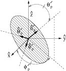
For the plate-hemisphere configuration shown in Figure 8, it can be shown that the element $\vec{R}_{p}$ on the plane and its velocity $d\vec{R}_{p}/dt$ are given by (see Appendix C3 of reference key-Sung-Nae-Cho ):

$\displaystyle\vec{R}_{p}\left(\grave{\vec{\Lambda}}_{p},\vec{\Lambda}^{\prime}_{p},\vec{R}_{T,p}\right)$
$\displaystyle=\left\{\sum_{i=1}^{3}\left[\nu_{T,p,i}+\nu^{\prime}_{p,\theta^{\prime}_{p}}\frac{\partial\Lambda^{\prime}_{p,i}}{\partial\theta^{\prime}_{p}}+\frac{\nu^{\prime}_{p,\phi^{\prime}_{p}}}{\sin\theta^{\prime}_{p}}\frac{\partial\Lambda^{\prime}_{p,i}}{\partial\phi^{\prime}_{p}}\right]^{2}\right\}^{1/2}$
$\displaystyle\times\sum_{i=1}^{3}\grave{\Lambda}_{p,i}\hat{e_{i}}$ (48)

and

$\displaystyle\dot{\vec{R}}_{p}$ $\displaystyle\equiv\frac{d\vec{R}_{p}}{dt}$
$\displaystyle=\left\{\sum_{i=1}^{3}\left[\nu_{T,p,i}+\nu^{\prime}_{p,\theta^{\prime}_{p}}\frac{\partial\Lambda^{\prime}_{p,i}}{\partial\theta^{\prime}_{p}}+\frac{\nu^{\prime}_{p,\phi^{\prime}_{p}}}{\sin\theta^{\prime}_{p}}\frac{\partial\Lambda^{\prime}_{p,i}}{\partial\phi^{\prime}_{p}}\right]^{2}\right\}^{-1/2}$
$\displaystyle\times\sum_{j=1}^{3}\sum_{k=1}^{3}\left(\left[\nu_{T,p,k}+\nu^{\prime}_{p,\theta^{\prime}_{p}}\frac{\partial\Lambda^{\prime}_{p,k}}{\partial\theta^{\prime}_{p}}+\frac{\nu^{\prime}_{p,\phi^{\prime}_{p}}}{\sin\theta^{\prime}_{p}}\frac{\partial\Lambda^{\prime}_{p,k}}{\partial\phi^{\prime}_{p}}\right]\right.$
$\displaystyle\times\left[\dot{\nu}_{T,p,k}+\left\{\nu^{\prime}_{p,\theta^{\prime}_{p}}\frac{\partial^{2}\Lambda^{\prime}_{p,k}}{\partial\left[\theta^{\prime}_{p}\right]^{2}}+\frac{\nu^{\prime}_{p,\phi^{\prime}_{p}}}{\sin\theta^{\prime}_{p}}\left(\frac{\partial^{2}\Lambda^{\prime}_{p,k}}{\partial\theta^{\prime}_{p}\partial\phi^{\prime}_{p}}\right.\right.\right.$
$\displaystyle\left.\left.-\cot\theta^{\prime}_{p}\frac{\partial\Lambda^{\prime}_{p,k}}{\partial\phi^{\prime}_{p}}\right)\right\}\dot{\theta^{\prime}}_{p}+\left\{\nu^{\prime}_{p,\theta^{\prime}_{p}}\frac{\partial^{2}\Lambda^{\prime}_{p,k}}{\partial\phi^{\prime}_{p}\partial\theta^{\prime}_{p}}+\frac{\nu^{\prime}_{p,\phi^{\prime}_{p}}}{\sin\theta^{\prime}_{p}}\right.$
$\displaystyle\left.\left.\times\frac{\partial^{2}\Lambda^{\prime}_{p,k}}{\partial\left[\phi^{\prime}_{p}\right]^{2}}\right\}\dot{\phi^{\prime}}_{p}+\dot{\nu^{\prime}}_{p,\theta^{\prime}_{p}}\frac{\partial\Lambda^{\prime}_{p,k}}{\partial\theta^{\prime}_{p}}+\frac{\dot{\nu^{\prime}}_{p,\phi^{\prime}_{p}}}{\sin\theta^{\prime}_{p}}\frac{\partial\Lambda^{\prime}_{p,k}}{\partial\phi^{\prime}_{p}}\right]$
$\displaystyle\times\grave{\Lambda}_{p,j}+\sum_{i=1}^{3}\left[\nu_{T,p,i}+\nu^{\prime}_{p,\theta^{\prime}_{p}}\frac{\partial\Lambda^{\prime}_{p,i}}{\partial\theta^{\prime}_{p}}+\frac{\nu^{\prime}_{p,\phi^{\prime}_{p}}}{\sin\theta^{\prime}_{p}}\frac{\partial\Lambda^{\prime}_{p,i}}{\partial\phi^{\prime}_{p}}\right]^{2}$
$\displaystyle\left.\times\left[\frac{\partial\grave{\Lambda}_{p,j}}{\partial\grave{\theta}_{p}}\frac{\partial\grave{\theta}_{p}}{\partial\phi^{\prime}_{p}}\dot{\theta}^{\prime}_{p}+\frac{\partial\grave{\Lambda}_{p,j}}{\partial\grave{\phi}_{p}}\frac{\partial\grave{\phi}_{p}}{\partial\phi^{\prime}_{p}}\dot{\phi}^{\prime}_{p}\right]\right)\hat{e_{j}},$ (49)

where

$\displaystyle\grave{\phi}_{p}$ $\displaystyle\equiv\grave{\phi}_{p}\left(\theta^{\prime}_{p},\phi^{\prime}_{p},\nu_{T,p,1},\nu_{T,p,2}\right)$
$\displaystyle=\arctan\left(\frac{\nu_{T,p,2}+\sin\theta^{\prime}_{p}\sin\phi^{\prime}_{p}}{\nu_{T,p,1}+\sin\theta^{\prime}_{p}\cos\phi^{\prime}_{p}}\right),$ (50)
$\displaystyle\grave{\theta}_{p}$ $\displaystyle\equiv\grave{\theta}_{p}\left(\theta^{\prime}_{p},\phi^{\prime}_{p},\vec{R}_{T,p}\right)$
$\displaystyle=\arctan\left(\frac{\nu_{T,p,1}+\nu_{T,p,2}+\sin\theta^{\prime}_{p}\left[\cos\phi^{\prime}_{p}+\sin\phi^{\prime}_{p}\right]}{\nu_{T,p,3}+\cos\theta^{\prime}_{p}}\right.$
$\displaystyle\times\left\{\cos\left(\arctan\left(\frac{\nu_{T,p,2}+\sin\theta^{\prime}_{p}\sin\phi^{\prime}_{p}}{\nu_{T,p,1}+\sin\theta^{\prime}_{p}\cos\phi^{\prime}_{p}}\right)\right)\right.$
$\displaystyle\left.\left.+\sin\left(\arctan\left(\frac{\nu_{T,p,2}+\sin\theta^{\prime}_{p}\sin\phi^{\prime}_{p}}{\nu_{T,p,1}+\sin\theta^{\prime}_{p}\cos\phi^{\prime}_{p}}\right)\right)\right\}^{-1}\right),$ (51)

and

$$\left\{\begin{array}[]{c}\grave{\Lambda}_{p,1}\left(\grave{\theta}_{p},\grave{\phi}_{p}\right)=\sin\grave{\theta}_{p}\cos\grave{\phi}_{p},\\ \\ \grave{\Lambda}_{p,2}\left(\grave{\theta}_{p},\grave{\phi}_{p}\right)=\sin\grave{\theta}_{p}\sin\grave{\phi}_{p},\\ \\ \grave{\Lambda}_{p,3}\left(\grave{\theta}_{p}\right)=\cos\grave{\theta}_{p}.\end{array}\right.$$ (52)

The subscript $p$ of $\grave{\phi}_{p}$ and $\grave{\theta}_{p}$ indicates that these are spherical variables for the points on the plate of Figure 8, not that of the hemisphere. It is also understood that $\Lambda^{\prime}_{p,3}$ and $\grave{\Lambda}_{p,3}$ are independent of $\phi^{\prime}_{p}$ and $\grave{\phi}_{p},$ respectively. Therefore, their differentiation with respect to $\phi^{\prime}_{p}$ and $\grave{\phi}_{p}$ respectively vanishes. The quantities $\dot{\theta^{\prime}}_{p}$ and $\dot{\phi^{\prime}}_{p}$ are the angular frequencies, and $\dot{\nu}_{T,p,i}$ is the translation speed of the plate relative to the system origin. The quantities $\dot{\nu^{\prime}}_{p,\theta^{\prime}_{p}}$ and $\dot{\nu^{\prime}}_{p,\phi^{\prime}_{p}}$ are the lattice vibrations along the directions $\hat{\theta^{\prime}}_{p}$ and $\hat{\phi^{\prime}}_{p}$ respectively. For the static plate without lattice vibrations, $\dot{\nu^{\prime}}_{p,\theta^{\prime}_{p}}$ and $\dot{\nu^{\prime}}_{p,\phi^{\prime}_{p}}$ vanishes.

Refer to caption
Figure 8: The plate-hemisphere configuration.

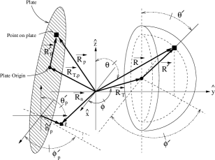
In the cross-sectional view of the plate-hemisphere system shown in Figure 9, the initial wave vector $\vec{k^{\prime}}_{i}$ traveling toward the hemisphere would go through a series of reflections according to the law of reflection and finally exit the cavity. It would then continue toward the plate, and depending on the orientation of plate at the time of impact, the wave-vector, now reflecting off the plate, would either escape to infinity or re-enter the hemisphere. The process repeats successively. In order to determine whether the wave that just escaped from the hemisphere cavity can reflect back from the plate and re-enter the hemisphere or escape to infinity, the exact location of reflection on the plate must be known. This reflection point on the plate is found to be (see Appendix C3 of reference key-Sung-Nae-Cho ),

$\displaystyle\vec{R}_{p}=$ $\displaystyle\left\{\sum_{s=1}^{3}\left[-\frac{\sum_{i=1}^{3}\frac{\partial\Lambda^{\prime}_{p,i}}{\partial\phi^{\prime}_{p}}\left(\Lambda^{\prime}_{p,i}+\frac{\epsilon_{ijk}k^{\prime}_{1,j}r^{\prime}_{0,k}}{\left\|\vec{n^{\prime}}_{p,1}\right\|}\right)}{\sum_{l=1}^{3}\frac{\partial\Lambda^{\prime}_{p,l}}{\partial\theta^{\prime}_{p}}\left(\Lambda^{\prime}_{p,l}+\frac{\epsilon_{lmn}k^{\prime}_{1,m}r^{\prime}_{0,n}}{\left\|\vec{n^{\prime}}_{p,1}\right\|}\right)}\right.\right.$
$\displaystyle\left.\left.\times\frac{\partial\Lambda^{\prime}_{p,s}}{\partial\theta^{\prime}_{p}}+\frac{\partial\Lambda^{\prime}_{p,s}}{\partial\phi^{\prime}_{p}}\right]^{2}\right\}^{1/2}\left[\frac{A_{\gamma}A_{\beta}}{C_{\beta}C_{\gamma}}+\frac{B_{\zeta}B_{\beta}}{C_{\beta}}\right.$
$\displaystyle\left.+\frac{\gamma_{o}B_{\gamma}A_{\beta}}{C_{\beta}C_{\gamma}}\right]\sum_{i=1}^{3}\grave{\Lambda}_{p,i}\hat{e_{i}},$ (53)

where the translation parameter $\nu_{T,p,j}=0;$ and the terms $\left(A_{\zeta},B_{\zeta},C_{\zeta}\right),$ $\left(A_{\gamma},B_{\gamma},C_{\gamma}\right),$ $\left(A_{\beta},B_{\beta},C_{\beta}\right)$ and $\gamma_{o}$ are defined as (see Appendix C3 of reference key-Sung-Nae-Cho ):

$$\left\{\begin{array}[]{c}A_{\zeta}=\sqrt{\sum_{j=1}^{3}\left[\nu_{T,h,j}+r^{\prime}_{i}\Lambda^{\prime}_{h,N_{h,max}+1,j}\right]^{2}},\\ \\ B_{\zeta}=\sqrt{\sum_{j=1}^{3}\left[\nu_{T,h,j}+r^{\prime}_{i}\Lambda^{\prime}_{h,N_{h,max},j}\right]^{2}},\\ \\ C_{\zeta}=-\left(\sum_{x=1}^{3}\frac{\partial\Lambda^{\prime}_{p,x}}{\partial\phi^{\prime}_{p}}\left[\Lambda^{\prime}_{p,x}+\frac{\epsilon_{xyz}k^{\prime}_{1,y}r^{\prime}_{0,z}}{\left\|\vec{n^{\prime}}_{p,1}\right\|}\right]\right)\\ \times\left(\sum_{l=1}^{3}\frac{\partial\Lambda^{\prime}_{p,l}}{\partial\theta^{\prime}_{p}}\left[\Lambda^{\prime}_{p,l}+\frac{\epsilon_{lmn}k^{\prime}_{1,m}r^{\prime}_{0,n}}{\left\|\vec{n^{\prime}}_{p,1}\right\|}\right]\right)^{-1};\end{array}\right.$$ (54)
$$\left\{\begin{array}[]{c}A_{\gamma}=\epsilon_{ijk}R_{h,N_{h,max},j}\left[R_{h,N_{h,max}+1,k}-R_{h,N_{h,max},k}\right],\\ \\ B_{\gamma}=\left\|\vec{n^{\prime}}_{p,1}\right\|^{-1}\epsilon_{ijk}k^{\prime}_{1,j}r^{\prime}_{0,k},\\ \\ C_{\gamma}=\epsilon_{ijk}\left[R_{h,N_{h,max},j}-R_{h,N_{h,max}+1,j}\right]\\ \times\left[R_{h,N_{h,max}+1,k}-R_{h,N_{h,max},k}\right];\end{array}\right.$$ (55)
$$\left\{\begin{array}[]{c}A_{\beta}=\sum_{i=1}^{3}\left[A_{\zeta}\grave{\Lambda}_{h,N_{h,max}+1,i}-B_{\zeta}\grave{\Lambda}_{h,N_{h,max},i}\right],\\ \\ B_{\beta}=\sum_{i=1}^{3}\grave{\Lambda}_{h,N_{h,max},i},\\ \\ C_{\beta}=\left\{\sum_{j=1}^{3}\left[\frac{\partial\Lambda^{\prime}_{p,j}}{\partial\phi^{\prime}_{p}}-C_{\zeta}\frac{\partial\Lambda^{\prime}_{p,j}}{\partial\theta^{\prime}_{p}}\right]^{2}\right\}^{1/2}\\ \times\sum_{l=1}^{3}\grave{\Lambda}_{p,l};\end{array}\right.$$ (56)
$\displaystyle\gamma_{o}$ $\displaystyle=\left(\left\|\vec{n^{\prime}}_{p,1}\right\|^{-1}\sum_{i=1}^{3}\epsilon_{ijk}k^{\prime}_{1,j}r^{\prime}_{0,k}-C_{\beta}^{-1}C_{\gamma}^{-1}\right.$
$\displaystyle\times B_{\gamma}A_{\beta}\sqrt{\sum_{j=1}^{3}\left[\frac{\partial\Lambda^{\prime}_{p,j}}{\partial\phi^{\prime}_{p}}-C_{\zeta}\frac{\partial\Lambda^{\prime}_{p,j}}{\partial\theta^{\prime}_{p}}\right]^{2}}$
$\displaystyle\left.\times\sum_{i=1}^{3}\epsilon_{ijk}\grave{\Lambda}_{p,j}k_{N_{h,max}+1,k}\right)^{-1}\left(\left[\frac{A_{\gamma}A_{\beta}}{C_{\beta}C_{\gamma}}\right.\right.$
$\displaystyle\left.+\frac{B_{\zeta}B_{\beta}}{C_{\beta}}\right]\sqrt{\sum_{j=1}^{3}\left[\frac{\partial\Lambda^{\prime}_{p,j}}{\partial\phi^{\prime}_{p}}-C_{\zeta}\frac{\partial\Lambda^{\prime}_{p,j}}{\partial\theta^{\prime}_{p}}\right]^{2}}$
$\displaystyle\left.\times\sum_{i=1}^{3}\epsilon_{ijk}\grave{\Lambda}_{p,j}k_{N_{h,max}+1,k}\right).$ (57)

It is to be noticed that for a situation where the translation parameter $\nu_{T,p,j}=0,$ the $\grave{\Lambda}$ becomes identical to $\Lambda^{\prime}$ in form. Results for $\grave{\Lambda}$ can be obtained from $\Lambda^{\prime}$ by a simple replacement of primed variables with the unprimed ones. It can be shown that the criterion whether the wave reflecting off the plate at location $\vec{R}_{p}$ can re-enter the hemisphere cavity or simply escape to infinity is found from the relation (see Appendix C3 of reference key-Sung-Nae-Cho ),

$\displaystyle\xi_{\kappa,i}$ $\displaystyle=\left(\nu_{T,h,i}+r^{\prime}_{0,i}-\left\{\sum_{s=1}^{3}\left[\frac{\partial\Lambda^{\prime}_{p,s}}{\partial\phi^{\prime}_{p}}-\frac{\partial\Lambda^{\prime}_{p,s}}{\partial\theta^{\prime}_{p}}\right.\right.\right.$
$\displaystyle\left.\left.\times\frac{\sum_{i=1}^{3}\frac{\partial\Lambda^{\prime}_{p,i}}{\partial\phi^{\prime}_{p}}\left(\Lambda^{\prime}_{p,i}+\frac{\epsilon_{ijk}k^{\prime}_{1,j}r^{\prime}_{0,k}}{\left\|\vec{n^{\prime}}_{p,1}\right\|}\right)}{\sum_{l=1}^{3}\frac{\partial\Lambda^{\prime}_{p,l}}{\partial\theta^{\prime}_{p}}\left(\Lambda^{\prime}_{p,l}+\frac{\epsilon_{lmn}k^{\prime}_{1,m}r^{\prime}_{0,n}}{\left\|\vec{n^{\prime}}_{p,1}\right\|}\right)}\right]^{2}\right\}^{1/2}$
$\displaystyle\left.\times\left[\frac{A_{\gamma}A_{\beta}}{C_{\beta}C_{\gamma}}+\frac{\gamma_{o}B_{\gamma}A_{\beta}}{C_{\beta}C_{\gamma}}+\frac{B_{\zeta}B_{\beta}}{C_{\beta}}\right]\grave{\Lambda}_{p,i}\right)$
$\displaystyle\times\left(\sum_{k=1}^{3}\left\{\alpha_{r,\perp}\left[k_{N_{h,max}+1,i}n^{\prime}_{p,k}n^{\prime}_{p,k}\right.\right.\right.$
$\displaystyle\left.-n^{\prime}_{p,i}k_{N_{h,max}+1,k}n^{\prime}_{p,k}\right]-\alpha_{r,\parallel}n^{\prime}_{p,k}$
$\displaystyle\left.\left.\times k_{N_{h,max}+1,k}n^{\prime}_{p,i}\right\}\right)^{-1},$ (58)

where $i=1,2,3$ and $\xi_{\kappa,i}$ is the component of the scale vector $\vec{\xi}_{\kappa}=\sum_{i=1}^{3}\xi_{\kappa,i}\hat{e_{i}}$ explained in the Appendix C3 of reference key-Sung-Nae-Cho .

Refer to caption
Figure 9: The intersection between oscillating plate, hemisphere and the plane of incidence whose normal is $\hat{n^{\prime}}_{p,1}=-\left\|\vec{n^{\prime}}_{p,1}\right\|^{-1}\sum_{i=1}^{3}\epsilon_{ijk}k^{\prime}_{1,j}r^{\prime}_{0,k}\hat{e_{i}}.$

In the above re-entry criteria, it should be noticed that $\vec{R}_{0}\leq r^{\prime}_{i}.$ This implies $r^{\prime}_{0,i}\leq r^{\prime}_{i},$ where $r^{\prime}_{i}$ is the radius of hemisphere. It is then concluded that all waves re-entering the hemisphere cavity would satisfy the condition $\xi_{\kappa,1}=\xi_{\kappa,2}=\xi_{\kappa,3}.$ On the other hand, those waves that escapes to infinity cannot have all three $\xi_{\kappa,i}$ equal to a single constant. The re-entry condition $\xi_{\kappa,1}=\xi_{\kappa,2}=\xi_{\kappa,3}$ is just another way of stating the existence of a parametric line along the vector $\vec{k}_{r,N_{h,max}+1}$ that happens to pierce through the hemisphere opening. In case such a line does not exist, the initial wave direction has to be rotated into a new direction such that there is a parametric line that pierces through the hemisphere opening. That is why all three $\xi_{\kappa,i}$ values cannot be equal to a single constant. The re-entry criteria are summarized here for bookkeeping purpose:

$$\left\{\begin{array}[]{c}\xi_{\kappa,1}=\xi_{\kappa,2}=\xi_{\kappa,3}:\quad wave\;reenters\;hemisphere,\\ \\ \;\;\;\qquad\qquad else:\quad wave\;escapes\;to\;infinity,\end{array}\right.$$ (59)

where $else$ is the case where $\xi_{\kappa,1}=\xi_{\kappa,2}=\xi_{\kappa,3}$ cannot be satisfied. The details of this section can be found in Appendix C3 of reference key-Sung-Nae-Cho .

II.3 Dynamical Casimir Force

The phenomenon of Casimir effect is inherently a dynamical effect due to the fact that it involves radiation, rather than static fields. One of our original objectives in studying the Casimir effect was to investigate the physical implications of vacuum-fields on movable boundaries. Consider the two parallel plates configuration of charge-neutral, perfect conductors shown in Figure 10. Because there are more wave modes in the outer region of the parallel plate resonator, two loosely restrained (or unfixed in position) plates will accelerate inward until they finally meet. The energy conservation would require that the energy initially confined in the resonator when the two plates were separated be transformed into the heat energy that acts to raise the temperatures of the two plates.

Refer to caption
Figure 10: Because there are more vacuum-field modes in the external regions, the two charge-neutral conducting plates are accelerated inward till the two finally stick.

Davies in 1975 key-Davies , followed by Unruh in 1976 key-Unruh , have asked the similar question and came to a conclusion that when an observer is moving with a constant acceleration in vacuum, the observer perceives himself to be immersed in a thermal bath at the temperature

$\displaystyle T$ $\displaystyle=\frac{\hbar\ddot{R}}{2\pi ck^{\prime}},$

where $\ddot{R}$ is the acceleration of the observer and $k^{\prime},$ the wave number. The details of the Unruh-Davies effect can also be found in the reference key-Milonni . The other work that dealt with the concept of dynamical Casimir effect is due to Schwinger in his proposals key-Milton ; key-Schwinger-Casimir-Light to explain the phenomenon of sonoluminescense. Sonoluminescense is a phenomenon in which when a small air bubble filled with noble gas is under a strong acoustic-field pressure, the bubble will emit an intense flash of light in the optical range.

Our formulation of dynamical Casimir effect here, however, has no resemblance to that of Schwinger’s work to the best of our knowledge. This formulation of dynamical Casimir force is briefly presented in the following sections. The details of derivations pertaining to the dynamical Casimir force can be found in Appendix D of reference key-Sung-Nae-Cho .

II.3.1 Formalism of Zero-Point Energy and its Force

For massless fields, the energy-momentum relation is

$\displaystyle\mathcal{H}^{\prime}_{n_{s}}$ $\displaystyle\equiv E_{Total}=pc,$ (60)

where $p$ is the momentum, $c$ is the speed of light, and $\mathcal{H}^{\prime}_{n_{s}}$ is the quantized field energy for the harmonic fields of equation (1) for the bounded space, or equation (2) for the free space. For the bounded space, the quantized field energy $\mathcal{H}^{\prime}_{n_{s}}\equiv\mathcal{H}^{\prime}_{n_{s},b}$ of equation (1) is a function of the wave number $k^{\prime}_{i}\left(n_{i}\right),$ which in turn is a function of the wave mode value $n_{i}$ and the boundary functional $f_{i}\left(L_{i}\right),$ where $L_{i}$ is the gap distance in the direction of

$\displaystyle\vec{L}_{i}$ $\displaystyle=\left[\vec{R^{\prime}}_{2}\cdot\hat{e}_{i}-\vec{R^{\prime}}_{1}\cdot\hat{e}_{i}\right]\hat{e}_{i}.$

Here $\vec{R^{\prime}}_{1}$ and $\vec{R^{\prime}}_{2}$ are the position vectors for the involved boundaries. As an illustration with the two plate configuration shown in Figure 10, $\vec{R^{\prime}}_{1}$ may represent the plate positioned at $z=0$ and $\vec{R^{\prime}}_{2}$ may correspond to the plate at the position $z=d.$ When the position of these boundaries are changing in time, the quantized field energy $\mathcal{H}^{\prime}_{n_{s}}\equiv\mathcal{H}^{\prime}_{n_{s},b}$ will be modified accordingly because the wave number functional $k^{\prime}_{i}\left(n_{i}\right)$ is varying in time,

$\displaystyle\frac{dk^{\prime}_{i}}{dt}$ $\displaystyle=\frac{\partial k^{\prime}_{i}}{\partial n_{i}}\frac{dn_{i}}{dt}f_{i}\left(L_{i}\right)+n_{i}\frac{\partial f_{i}}{\partial L_{i}}\frac{dL_{i}}{dt}$
$\displaystyle=f_{i}\left(L_{i}\right)\frac{\partial k^{\prime}_{i}}{\partial n_{i}}\dot{n}_{i}+n_{i}\frac{\partial f_{i}}{\partial L_{i}}\dot{L}_{i}.$

Here the term proportional to $\dot{n}_{i}$ refers to the case where the boundaries remain fixed throughout all times but the number of wave modes in the resonator are being driven by some active external influence. The term proportional to $\dot{L}_{i}$ represents the changes in the number of wave modes due to the moving boundaries.

For an isolated system, there are no external influences, hence $\dot{n}_{i}=0.$ The dynamical force arising from the time variation of the boundaries is found to be (see Appendix D1 of reference key-Sung-Nae-Cho ),

$\displaystyle\vec{\mathcal{F}^{\prime}}_{\alpha}$ $\displaystyle=\sum_{i=1}^{3}\left\{n_{i}\frac{\partial f_{i}}{\partial L_{i}}\left[C_{\alpha,5}\frac{\partial^{2}\mathcal{H}^{\prime}_{n_{s}}}{\partial\left[k^{\prime}_{i}\right]^{2}}+\left(1-\delta_{i\alpha}\right)\right.\right.$
$\displaystyle\left.\times\left(C_{\alpha,6}-C_{\alpha,7}\left[n_{s}+\frac{1}{2}\right]k^{\prime}_{i}\right)\left[n_{s}+\frac{1}{2}\right]\right]\dot{L}_{i}$
$\displaystyle\left.+\sum_{j=1}^{3}\left(1-\delta_{ij}\right)C_{\alpha,5}n_{j}\frac{\partial f_{j}}{\partial L_{j}}\frac{\partial^{2}\mathcal{H}^{\prime}_{n_{s}}}{\partial k^{\prime}_{j}\partial k^{\prime}_{i}}\dot{L}_{j}\right\}\hat{e_{\alpha}},$ (61)

where $C_{\alpha,1},$ $C_{\alpha,2},$ $C_{\alpha,3},$ $C_{\alpha,4},$ $C_{\alpha,5},$ $C_{\alpha,6}$ and $C_{\alpha,7}$ are defined as

$$\left\{\begin{array}[]{c}C_{\alpha,1}=\sum_{i=1}^{3}\frac{\partial\mathcal{H}^{\prime}_{n_{s}}}{\partial k^{\prime}_{i}},\\ \\ C_{\alpha,2}=\sum_{i=1}^{3}\left(1-\delta_{i\alpha}\right)\left(\left[n_{s}+\frac{1}{2}\right]\hbar c\right)^{2}k^{\prime}_{i},\\ \\ C_{\alpha,3}=\sum_{i=1}^{3}\left(1-\delta_{i\alpha}\right)\left(\left[n_{s}+\frac{1}{2}\right]\hbar\right)^{2}\left[k^{\prime}_{i}\right]^{2},\end{array}\right.$$ (62)
$\displaystyle C_{\alpha,4}$ $\displaystyle=\left(\frac{\left[n_{s}+\frac{1}{2}\right]^{2}\hbar^{2}C_{\alpha,2}^{2}}{\left[C_{\alpha,1}^{2}-\left(\left[n_{s}+\frac{1}{2}\right]\hbar c\right)^{2}\right]^{2}}\right.$
$\displaystyle\left.+\frac{C_{\alpha,2}^{2}-C_{\alpha,1}^{2}C_{\alpha,3}}{C_{\alpha,1}^{2}-\left(\left[n_{s}+\frac{1}{2}\right]\hbar c\right)^{2}}\right)^{-1/2},$ (63)
$\displaystyle C_{\alpha,5}$ $\displaystyle=\frac{C_{\alpha,1}C_{\alpha,4}\left[C_{\alpha,1}^{2}C_{\alpha,3}-C_{\alpha,2}^{2}\right]}{\left[C_{\alpha,1}^{2}-\left(\left[n_{s}+\frac{1}{2}\right]\hbar c\right)^{2}\right]^{2}}$
$\displaystyle-\frac{2\left[n_{s}+\frac{1}{2}\right]^{2}\hbar^{2}C_{\alpha,1}C_{\alpha,2}^{2}C_{\alpha,4}}{\left[C_{\alpha,1}^{2}-\left(\left[n_{s}+\frac{1}{2}\right]\hbar c\right)^{2}\right]^{3}}$
$\displaystyle-\frac{2\left[n_{s}+\frac{1}{2}\right]\hbar C_{\alpha,1}C_{\alpha,2}}{\left[C_{\alpha,1}^{2}-\left(\left[n_{s}+\frac{1}{2}\right]\hbar c\right)^{2}\right]^{2}}$
$\displaystyle-\frac{C_{\alpha,1}C_{\alpha,3}C_{\alpha,4}}{C_{\alpha,1}^{2}-\left(\left[n_{s}+\frac{1}{2}\right]\hbar c\right)^{2}},$ (64)
$\displaystyle C_{\alpha,6}$ $\displaystyle=\frac{\left[n_{s}+\frac{1}{2}\right]^{2}\hbar^{2}C_{\alpha,2}C_{\alpha,4}}{\left[C_{\alpha,1}^{2}-\left(\left[n_{s}+\frac{1}{2}\right]\hbar c\right)^{2}\right]^{2}}$
$\displaystyle+\frac{C_{\alpha,2}C_{\alpha,4}}{C_{\alpha,1}^{2}-\left(\left[n_{s}+\frac{1}{2}\right]\hbar c\right)^{2}}$
$\displaystyle+\frac{\left[n_{s}+\frac{1}{2}\right]\hbar}{C_{\alpha,1}^{2}-\left(\left[n_{s}+\frac{1}{2}\right]\hbar c\right)^{2}},$ (65)
$\displaystyle C_{\alpha,7}$ $\displaystyle=\frac{C_{\alpha,1}^{2}C_{\alpha,4}}{C_{\alpha,1}^{2}-\left(\left[n_{s}+\frac{1}{2}\right]\hbar c\right)^{2}}.$ (66)

The force shown in the above expression vanishes for the one dimensional case. This is an expected result. To understand why the force vanishes, we have to refer to the starting point equation,

$\displaystyle\sum_{i=1}^{3}\left[\left(\left[n_{s}+\frac{1}{2}\right]\hbar\right)^{-1}\frac{\partial\mathcal{H}^{\prime}_{n_{s}}}{\partial k^{\prime}_{i}}\right.$
$\displaystyle\left.-\left\{\sum_{i=1}^{3}\left[p^{\prime}_{i}\right]^{2}\right\}^{-1/2}cp^{\prime}_{i}\right]dp^{\prime}_{i}$ $\displaystyle=0,$ (67)

of the Appendix D1 of reference key-Sung-Nae-Cho . The summation here obviously runs only once to arrive at the expression, $\partial\mathcal{H}^{\prime}_{n_{s}}/\partial k^{\prime}_{i}=\left[n_{s}+\frac{1}{2}\right]\hbar c.$ This is a classic situation where the problem has been over specified. For the 3D case, equation (67) is a combination of two constraints, $\sum_{i=1}^{3}\left[p^{\prime}_{i}\right]^{2}$ and $\mathcal{H}^{\prime}_{n_{s}}.$ For the one dimensional case, there is only one constraint, $\mathcal{H}^{\prime}_{n_{s}}.$ Therefore, equation (67) becomes an over specification. In order to avoid the problem caused by over specifications in this formulation, the one dimensional force expression can be obtained directly by differentiating the equation (60) instead of using the above formulation for the three dimensional case. The 1D dynamical force expression for an isolated, non-driven systems then becomes

$\displaystyle\vec{\mathcal{F}^{\prime}}$ $\displaystyle=\frac{n}{c}\frac{\partial f}{\partial L}\frac{\partial\mathcal{H}^{\prime}_{n_{s}}}{\partial k^{\prime}}\dot{L}\hat{e},$ (68)

where $\vec{\mathcal{F}^{\prime}}$ is an one dimensional force. Here the subscript $\alpha$ of $\vec{\mathcal{F}^{\prime}}_{\alpha}$ have been dropped for simplicity, since it is a one dimensional force. The details of this section can be found in Appendix D1 of reference key-Sung-Nae-Cho .

II.3.2 Equations of Motion for the Driven Parallel Plates

The Unruh-Davies effect states that heating up of an accelerating conductor plate is proportional to its acceleration through the relation

$\displaystyle T$ $\displaystyle=\frac{\hbar\ddot{R}}{2\pi ck^{\prime}},$

where $\ddot{R}$ is the plate acceleration. A one dimensional system of two parallel plates, shown in Figure 11, can be used as a simple model to demonstrate the complicated sonoluminescense phenomenon for a bubble subject to a strong acoustic field.

Refer to caption
Figure 11: A one dimensional driven parallel plates configuration.

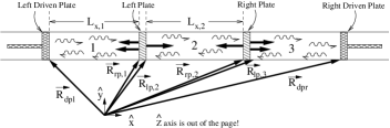
The dynamical force for the 1D, linear coupled system can be expressed with equation (68),

$\displaystyle\left\{\begin{array}[]{c}\ddot{R}_{1}-\eta_{1}\dot{R}_{1}-\eta_{2}\dot{R}_{2}=\xi_{rp},\\ \\ \ddot{R}_{2}-\eta_{3}\dot{R}_{2}-\eta_{4}\dot{R}_{1}=\xi_{lp},\end{array}\right.$ (72)

where

$$\left\{\begin{array}[]{c}\eta_{1}=m_{rp}^{-1}\left[s_{rp,2}g_{\alpha,2}-s_{rp,3}g_{\alpha,3}\right],\\ \\ \eta_{2}=-s_{rp,2}g_{\alpha,2}m_{rp}^{-1}\\ \\ \eta_{3}=m_{lp}^{-1}\left[s_{lp,1}g_{\alpha,1}-s_{lp,2}g_{\alpha,2}\right],\\ \\ \eta_{4}=s_{lp,2}g_{\alpha,2}m_{lp}^{-1},\\ \\ \xi_{rp}=s_{rp,3}g_{\alpha,3}m_{rp}^{-1}\dot{R}_{dpr,cm,\alpha},\\ \\ \xi_{lp}=-s_{lp,1}g_{\alpha,1}m_{lp}^{-1},\\ \\ R_{1}=R_{rp,cm,\alpha},\\ \\ R_{2}=R_{lp,cm,\alpha},\end{array}\right.$$ (73)
$\displaystyle\dot{R}_{a,b}=\frac{d\vec{R}_{a}}{dt}\cdot\hat{e_{b}},$ $\displaystyle\ddot{R}_{a,b}=\frac{d^{2}\vec{R}_{a}}{dt^{2}}\cdot\hat{e_{b}},$
$\displaystyle g_{\alpha,\Re}$ $\displaystyle=\frac{n_{\alpha,\Re}}{c}\left(\frac{\partial f_{\alpha,\Re}}{\partial L_{\alpha,\Re}}\right)\left(\frac{\partial\mathcal{H}^{\prime}_{n_{s},\Re}}{\partial k^{\prime}_{\alpha,\Re}}\right).$ (74)

Here $R_{1}$ represents the center of mass position for the “Right Plate” and $R_{2}$ represents the center of mass position for the “Left Plate” as illustrated in Figure 11. $m_{rp}$ and $m_{lp}$ are the corresponding masses for the right and left plates. $s_{rp,i}$ and $s_{lp,i}$ are the appropriate $\left(\pm\right)$signs that needs to be determined. For the mean time, the exact signs for $s_{rp,i}$ and $s_{lp,i}$ are not relevant, hence it is left as is. With a slight modification, equation (72) for this linear coupled system can be written in the matrix form, (see Appendix D2 of reference key-Sung-Nae-Cho ):

$\displaystyle R_{1}=\int_{t_{0}}^{t}R_{3}dt^{\prime},$ $\displaystyle R_{2}=\int_{t_{0}}^{t}R_{4}dt^{\prime},$

and

$\displaystyle\underbrace{\left[\begin{array}[]{c}\dot{R}_{3}\\ \dot{R}_{4}\end{array}\right]}_{\dot{\vec{R}}_{\eta}}$ $\displaystyle=\underbrace{\left[\begin{array}[]{cc}\eta_{1}&\eta_{2}\\ \eta_{4}&\eta_{3}\end{array}\right]}_{\widetilde{M}_{\eta}}\underbrace{\left[\begin{array}[]{c}R_{3}\\ R_{4}\end{array}\right]}_{\vec{R}_{\eta}}+\underbrace{\left[\begin{array}[]{c}\xi_{rp}\\ \xi_{lp}\end{array}\right]}_{\vec{\xi}},$ (83)

where

$$\left\{\begin{array}[]{c}\begin{array}[]{ccc}\dot{R}_{1}=R_{3},&&\dot{R}_{2}=R_{4},\\ \end{array}\\ \dot{R}_{3}=\ddot{R}_{1}=\xi_{rp}+\eta_{1}\dot{R}_{1}+\eta_{2}\dot{R}_{2}=\xi_{rp}+\eta_{1}R_{3}+\eta_{2}R_{4},\\ \\ \dot{R}_{4}=\ddot{R}_{2}=\xi_{lp}+\eta_{3}\dot{R}_{2}+\eta_{4}\dot{R}_{1}=\xi_{lp}+\eta_{3}R_{4}+\eta_{4}R_{3}.\end{array}\right.$$

The matrix equation has the solutions (see Appendix D2 of reference key-Sung-Nae-Cho ):

$\displaystyle\dot{R}_{rp,cm,\alpha}\left(t\right)=\left[\frac{\lambda_{4}\left(;t_{0}\right)-\eta_{1}\left(;t_{0}\right)}{\lambda_{3}\left(;t_{0}\right)-\eta_{1}\left(;t_{0}\right)}-1\right]^{-1}$
$\displaystyle\times\frac{\psi_{11}\left(t,t_{0}\right)\dot{R}_{rp,cm,\alpha}\left(t_{0}\right)+\psi_{12}\left(t,t_{0}\right)\dot{R}_{lp,cm,\alpha}\left(t_{0}\right)}{\exp\left(\left[\lambda_{3}\left(;t_{0}\right)+\lambda_{4}\left(;t_{0}\right)\right]t_{0}\right)}$
$\displaystyle+\int_{t_{0}}^{t}\frac{\psi_{22}\left(t^{\prime},t_{0}\right)\xi_{rp}\left(t^{\prime}\right)-\psi_{12}\left(t^{\prime},t_{0}\right)\xi_{lp}\left(t^{\prime}\right)}{\psi_{11}\left(t^{\prime},t_{0}\right)\psi_{22}\left(t^{\prime},t_{0}\right)-\psi_{12}\left(t^{\prime},t_{0}\right)\psi_{21}\left(t^{\prime},t_{0}\right)}dt^{\prime}$
$\displaystyle\times\psi_{11}\left(t,t_{0}\right)+\psi_{12}\left(t,t_{0}\right)$
$\displaystyle\times\int_{t_{0}}^{t}\frac{\psi_{11}\left(t^{\prime},t_{0}\right)\xi_{lp}\left(t^{\prime}\right)-\psi_{21}\left(t^{\prime},t_{0}\right)\xi_{rp}\left(t^{\prime}\right)}{\psi_{11}\left(t^{\prime},t_{0}\right)\psi_{22}\left(t^{\prime},t_{0}\right)-\psi_{12}\left(t^{\prime},t_{0}\right)\psi_{21}\left(t^{\prime},t_{0}\right)}dt^{\prime},$ (84)
$\displaystyle\dot{R}_{lp,cm,\alpha}\left(t\right)=\left[\frac{\lambda_{4}\left(;t_{0}\right)-\eta_{1}\left(;t_{0}\right)}{\lambda_{3}\left(;t_{0}\right)-\eta_{1}\left(;t_{0}\right)}-1\right]^{-1}$
$\displaystyle\times\frac{\psi_{21}\left(t,t_{0}\right)\dot{R}_{rp,cm,\alpha}+\psi_{22}\left(t,t_{0}\right)\dot{R}_{lp,cm,\alpha}\left(t_{0}\right)}{\exp\left(\left[\lambda_{3}\left(;t_{0}\right)+\lambda_{4}\left(;t_{0}\right)\right]t_{0}\right)}$
$\displaystyle+\int_{t_{0}}^{t}\frac{\psi_{22}\left(t^{\prime},t_{0}\right)\xi_{rp}\left(t^{\prime}\right)-\psi_{12}\left(t^{\prime},t_{0}\right)\xi_{lp}\left(t^{\prime}\right)}{\psi_{11}\left(t^{\prime},t_{0}\right)\psi_{22}\left(t^{\prime},t_{0}\right)-\psi_{12}\left(t^{\prime},t_{0}\right)\psi_{21}\left(t^{\prime},t_{0}\right)}dt^{\prime}$
$\displaystyle\times\psi_{21}\left(t,t_{0}\right)+\psi_{22}\left(t,t_{0}\right)$
$\displaystyle\times\int_{t_{0}}^{t}\frac{\psi_{11}\left(t^{\prime},t_{0}\right)\xi_{lp}\left(t^{\prime}\right)-\psi_{21}\left(t^{\prime},t_{0}\right)\xi_{rp}\left(t^{\prime}\right)}{\psi_{11}\left(t^{\prime},t_{0}\right)\psi_{22}\left(t^{\prime},t_{0}\right)-\psi_{12}\left(t^{\prime},t_{0}\right)\psi_{21}\left(t^{\prime},t_{0}\right)}dt^{\prime},$ (85)

where

$\displaystyle\lambda_{3}$ $\displaystyle=\frac{\eta_{1}+\eta_{3}}{2}+\sqrt{\frac{1}{4}\left[\eta_{1}-\eta_{3}\right]^{2}+\eta_{2}\eta_{4}},$ (86)
$\displaystyle\lambda_{4}$ $\displaystyle=\frac{\eta_{1}+\eta_{3}}{2}-\sqrt{\frac{1}{4}\left[\eta_{1}-\eta_{3}\right]^{2}+\eta_{2}\eta_{4}},$ (87)
$\displaystyle\psi_{11}\left(t,t_{0}\right)$ $\displaystyle=\grave{R}_{3}\grave{R}_{4}\left[\frac{\lambda_{4}-\eta_{1}}{\lambda_{3}-\eta_{1}}\exp\left(\lambda_{3}t+\lambda_{4}t_{0}\right)\right.$
$\displaystyle\left.-\exp\left(\lambda_{4}t+\lambda_{3}t_{0}\right)\right],$ (88)
$\displaystyle\psi_{12}\left(t,t_{0}\right)$ $\displaystyle=\grave{R}_{3}\grave{R}_{4}\left[\frac{\eta_{2}}{\lambda_{3}-\eta_{1}}\exp\left(\lambda_{4}t+\lambda_{3}t_{0}\right)\right.$
$\displaystyle\left.-\frac{\eta_{2}}{\lambda_{3}-\eta_{1}}\exp\left(\lambda_{3}t+\lambda_{4}t_{0}\right)\right],$ (89)
$\displaystyle\psi_{21}\left(t,t_{0}\right)$ $\displaystyle=\grave{R}_{3}\grave{R}_{4}\left[\frac{\lambda_{4}-\eta_{1}}{\eta_{2}}\exp\left(\lambda_{3}t+\lambda_{4}t_{0}\right)\right.$
$\displaystyle\left.-\frac{\lambda_{4}-\eta_{1}}{\eta_{2}}\exp\left(\lambda_{4}t+\lambda_{3}t_{0}\right)\right],$ (90)
$\displaystyle\psi_{22}\left(t,t_{0}\right)$ $\displaystyle=\grave{R}_{3}\grave{R}_{4}\left[\frac{\lambda_{4}-\eta_{1}}{\lambda_{3}-\eta_{1}}\exp\left(\lambda_{4}t+\lambda_{3}t_{0}\right)\right.$
$\displaystyle\left.-\exp\left(\lambda_{3}t+\lambda_{4}t_{0}\right)\right].$ (91)

The quantities $\dot{R}_{rp,cm,\alpha}$ and $\dot{R}_{lp,cm,\alpha}$ are the speed of the center of mass of “Right Plate” and the speed of the center of mass of the “Left Plate,” respectively, and $\alpha$ defines the particular basis direction. The corresponding positions $R_{rp,cm,\alpha}\left(t\right)$ and $R_{lp,cm,\alpha}\left(t\right)$ are found by integrating equations (84) and (85) with respect to time,

$\displaystyle R_{rp,cm,\alpha}\left(t\right)=\left[\frac{\lambda_{4}\left(;t_{0}\right)-\eta_{1}\left(;t_{0}\right)}{\lambda_{3}\left(;t_{0}\right)-\eta_{1}\left(;t_{0}\right)}-1\right]^{-1}$
$\displaystyle\times\int_{t_{0}}^{t}\left[\frac{\psi_{11}\left(\tau,t_{0}\right)\dot{R}_{rp,cm,\alpha}\left(t_{0}\right)+\psi_{12}\left(\tau,t_{0}\right)\dot{R}_{lp,cm,\alpha}\left(t_{0}\right)}{\exp\left(\left[\lambda_{3}\left(;t_{0}\right)+\lambda_{4}\left(;t_{0}\right)\right]t_{0}\right)}\right.$
$\displaystyle+\int_{t_{0}}^{\tau}\frac{\psi_{22}\left(t^{\prime},t_{0}\right)\xi_{rp}\left(t^{\prime}\right)-\psi_{12}\left(t^{\prime},t_{0}\right)\xi_{lp}\left(t^{\prime}\right)}{\psi_{11}\left(t^{\prime},t_{0}\right)\psi_{22}\left(t^{\prime},t_{0}\right)-\psi_{12}\left(t^{\prime},t_{0}\right)\psi_{21}\left(t^{\prime},t_{0}\right)}dt^{\prime}$
$\displaystyle\times\psi_{11}\left(\tau,t_{0}\right)+\psi_{12}\left(\tau,t_{0}\right)$
$\displaystyle\left.\times\int_{t_{0}}^{\tau}\frac{\psi_{11}\left(t^{\prime},t_{0}\right)\xi_{lp}\left(t^{\prime}\right)-\psi_{21}\left(t^{\prime},t_{0}\right)\xi_{rp}\left(t^{\prime}\right)}{\psi_{11}\left(t^{\prime},t_{0}\right)\psi_{22}\left(t^{\prime},t_{0}\right)-\psi_{12}\left(t^{\prime},t_{0}\right)\psi_{21}\left(t^{\prime},t_{0}\right)}dt^{\prime}\right]$
$\displaystyle\times d\tau+R_{rp,cm,\alpha}\left(t_{0}\right),$ (92)
$\displaystyle R_{lp,cm,\alpha}\left(t\right)=\left[\frac{\lambda_{4}\left(;t_{0}\right)-\eta_{1}\left(;t_{0}\right)}{\lambda_{3}\left(;t_{0}\right)-\eta_{1}\left(;t_{0}\right)}-1\right]^{-1}$
$\displaystyle\times\int_{t_{0}}^{t}\left[\frac{\psi_{21}\left(\tau,t_{0}\right)\dot{R}_{rp,cm,\alpha}\left(t_{0}\right)+\psi_{22}\left(\tau,t_{0}\right)\dot{R}_{lp,cm,\alpha}\left(t_{0}\right)}{\exp\left(\left[\lambda_{3}\left(;t_{0}\right)+\lambda_{4}\left(;t_{0}\right)\right]t_{0}\right)}\right.$
$\displaystyle+\int_{t_{0}}^{\tau}\frac{\psi_{22}\left(t^{\prime},t_{0}\right)\xi_{rp}\left(t^{\prime}\right)-\psi_{12}\left(t^{\prime},t_{0}\right)\xi_{lp}\left(t^{\prime}\right)}{\psi_{11}\left(t^{\prime},t_{0}\right)\psi_{22}\left(t^{\prime},t_{0}\right)-\psi_{12}\left(t^{\prime},t_{0}\right)\psi_{21}\left(t^{\prime},t_{0}\right)}dt^{\prime}$
$\displaystyle\times\psi_{21}\left(\tau,t_{0}\right)+\psi_{22}\left(\tau,t_{0}\right)$
$\displaystyle\left.\times\int_{t_{0}}^{\tau}\frac{\psi_{11}\left(t^{\prime},t_{0}\right)\xi_{lp}\left(t^{\prime}\right)-\psi_{21}\left(t^{\prime},t_{0}\right)\xi_{rp}\left(t^{\prime}\right)}{\psi_{11}\left(t^{\prime},t_{0}\right)\psi_{22}\left(t^{\prime},t_{0}\right)-\psi_{12}\left(t^{\prime},t_{0}\right)\psi_{21}\left(t^{\prime},t_{0}\right)}dt^{\prime}\right]$
$\displaystyle\times d\tau+R_{lp,cm,\alpha}\left(t_{0}\right).$ (93)

The remaining integrations are straightforward and the explicit forms will not be shown here.

One may argue that for the static case, $\dot{R}_{rp,cm,\alpha}\left(t_{0}\right)$ and $\dot{R}_{lp,cm,\alpha}\left(t_{0}\right)$ must be zero because the conductors seem to be fixed in position. This argument is flawed, for any wall totally fixed in position upon impact would require an infinite amount of energy. One has to consider the conservation of momentum simultaneously. The wall has to have moved by the amount $\bigtriangleup R_{wall}=\dot{R}_{wall}\triangle t,$ where $\triangle t$ is the total duration of impact, and $\dot{R}_{wall}$ is calculated from the momentum conservation and it is non-zero. The same argument can be applied to the apparatus shown in Figure 11. For that system

$\displaystyle\left\|\vec{p}_{virtual-photon}\right\|$ $\displaystyle=\frac{1}{c}\mathcal{H}^{\prime}_{n_{s},\Re}\left(t_{0}\right)$

and

$$\left\{\begin{array}[]{c}\dot{R}_{rp,cm,\alpha}\left(t_{0}\right)=\left\|\dot{\vec{R}}_{lp,3}\left(t_{0}\right)+\dot{\vec{R}}_{rp,2}\left(t_{0}\right)\right\|,\\ \\ \dot{R}_{lp,cm,\alpha}\left(t_{0}\right)=\left\|\dot{\vec{R}}_{rp,1}\left(t_{0}\right)+\dot{\vec{R}}_{lp,2}\left(t_{0}\right)\right\|.\end{array}\right.$$

For simplicity, assuming that the impact is always only in the normal direction,

$\displaystyle\dot{R}_{rp,cm,\alpha}\left(t_{0}\right)$ $\displaystyle=\frac{2}{m_{rp}c}\left\|\mathcal{H}^{\prime}_{n_{s},3}\left(t_{0}\right)-\mathcal{H}^{\prime}_{n_{s},2}\left(t_{0}\right)\right\|$

and

$\displaystyle\dot{R}_{lp,cm,\alpha}\left(t_{0}\right)$ $\displaystyle=\frac{2}{m_{lp}c}\left\|\mathcal{H}^{\prime}_{n_{s},1}\left(t_{0}\right)-\mathcal{H}^{\prime}_{n_{s},2}\left(t_{0}\right)\right\|,$

where the differences under the magnitude symbol imply field energies from different regions counteract the other. The details of this section can be found in Appendix D2 of reference key-Sung-Nae-Cho .

III Results and Outlook

The results for the sign of Casimir force on non-planar geometric configurations considered in this investigation will eventually be compared with the classic repulsive result obtained by Boyer decades earlier. For this reason, it is worth reviewing Boyer’s original configuration as shown in Figure 12.

Refer to caption
Figure 12: Boyer’s configuration is such that a sphere is the only matter in the entire universe. His universe extends to the infinity, hence there are no boundaries. The sense of vacuum-field energy flow is along the radial vector $\hat{r},$ which is defined with respect to the sphere center.

T. H. Boyer in 1968 obtained a repulsive Casimir force result for his charge-neutral, hollow spherical shell of a perfect conductor key-Boyer . For simplicity, his sphere is the only object in the entire universe and, therefore, no external boundaries such as laboratory walls, etc., were defined in his problem. Furthermore, the zero-point energy flow is always perpendicular to his sphere. Such restriction constitutes a very stringent condition for the material property that a sphere has to meet. For example, if one were to look at Boyer’s sphere, he would not see the whole sphere; but instead, he would see a small spot on the surface of a sphere that happens to be in his line of sight. This happens because the sphere in Boyer’s configuration can only radiate in a direction normal to the surface. One could equivalently argue that Boyer’s sphere only responds to the approaching radiation at normal angles of incidence with respect to the surface of the sphere. When the Casimir force is computed for such restricted radiation energy flow, the result is repulsive. In Boyer’s picture, this may be attributed to the fact that closer to the origin of a sphere, the spherically symmetric radiation energy flow becomes more dense due to the inverse length dependence, and this density decreases as it gets further away from the sphere center. This argument, however, seems to be flawed because it inherently implies existence of the preferred origin for the vacuum fields. As an illustration, Boyer’s sphere is shown in Figure 12. For the rest of this investigation, “Boyer’s sphere” would be strictly referred to as the sphere made of material with such a property that it only radiates or responds to vacuum-field radiations at normal angle of incidence with respect to its surface.

Refer to caption
Figure 13: Manufactured sphere, in which two hemispheres are brought together, results in small non-spherically symmetric vacuum-field radiation inside the cavity due to the configuration change. For the hemispheres made of Boyer’s material, these fields in the resonator will eventually get absorbed by the conductor resulting in heating of the hemispheres.

The formation of a sphere by bringing together two nearby hemispheres satisfying the material property of Boyer’s sphere is illustrated in Figure 13. Since Boyer’s material property only allow radiation in the normal direction to its surface, the radiation associated with each hemisphere would necessarily go through the corresponding hemisphere centers. For clarity, let us define the unit radial basis vector associated with the left and right hemispheres by $\hat{r}_{L}$ and $\hat{r}_{R},$ respectively. If the hemispheres are made of normal conductors the radiation from one hemisphere entering the other hemisphere cavity would go through a complex series of reflections before escaping the cavity. Here, a conductor with Boyer’s stringent material property is not considered normal. Conductors that are normal also radiate in directions non-normal to their surface, whereas Boyer’s conductor can only radiate normal to its surface. Due to the fact that Boyer’s conducting materials can only respond to radiation impinging at a normal angle of incidence with respect to its surface, all of the incoming radiation at oblique angles of incidence with respect to the local surface normal is absorbed by the host hemisphere. This suggests that for the hemisphere-hemisphere arrangement made of Boyer’s material shown in Figure 13, the temperature of the two hemispheres would rise indefinitely over time. This does not happen with ordinary conductors. This suggests that Boyer’s conducting material, of which his sphere is made, is completely hypothetical. Precisely because of this material assumption, Boyer’s Casimir force is repulsive.

Refer to caption
Figure 14: The process in which a configuration change from hemisphere-hemisphere to sphere inducing virtual photon in the direction other than $\hat{r}$ is shown. The virtual photon here is referred to as the quanta of energy associated with the zero-point radiation.

For the moment, let us relax the stringent Boyer’s material property for the hemispheres to that of ordinary conductors. For the hemispheres made of ordinary conducting materials, there would result a series of reflections in one hemisphere cavity due to those radiations entering the cavity from nearby hemisphere. For simplicity, the ordinary conducting material referred to here is that of perfect conductors without Boyer’s hypothetical material property requirement. Furthermore, only the radiation emanating normally with respect to its surface is considered. The idea is to illustrate that the “normally emanated radiation” from one hemisphere results in elaboration of the effects of “obliquely emanated radiation” on another hemisphere cavity. Here the obliquely emanated radiation means those radiation emanating from a surface not along the local normal of the surface.

When two such hemispheres are brought together to form a sphere, there would exist some radiation trapped in the sphere of which the radiation energy flow lines are not spherically symmetric with respect to the sphere center. To see how a mere change in configuration invokes such non-spherically symmetric energy flow, consider the illustration shown in Figure 14. For clarity, only one “normally emanated radiation” energy flow line from the left hemisphere is shown. When one brings together the two hemispheres just in time before that quantum of energy escapes the hemisphere cavity to the right, the trapped energy quantum would continuously go through series of complex reflections in the cavity obeying the reflection law. But how fast or how slow one brings in two hemispheres is irrelevant in invoking such non-spherically symmetric energy flow because the gap $\delta$ can be chosen arbitrarily. Therefore, there would always be a stream of energy quanta crossing the hemisphere opening with $\xi\neq 0$ as shown in Figure 14. In other words, there is always a time interval $\triangle t$ within which the hemispheres are separated by an amount $\delta$ before closure. The quanta of vacuum-field radiation energy created within that time interval $\triangle t$ would always be satisfying the condition $\xi\neq 0,$ and this results in reflections at oblique angle of incidence with respect to the local normal of the walls of inner sphere cavity. Only when the two hemispheres are finally closed, would then $\xi=0$ and the radiation energy produced in the sphere after that moment would be spherically symmetric and the reflections would be normal to the surface. However, those trapped quantum of energy that were produced prior to the closure of the two hemispheres would always be reflecting from the inner sphere surface at oblique angles of incidence.

Refer to caption
Figure 15: A realistic laboratory has boundaries, e.g., walls. These boundaries have effect similar to the field modes between two parallel plates. In 3D, the effects are similar to that of a cubical laboratory, etc.

Unlike Boyer’s ideal laboratory, realistic laboratories have boundaries made of ordinary material as illustrated in Figure 15. One must then take into account, when calculating the Casimir force, the vacuum-field radiation pressure contributions from the involved conductors, as well as those contributions from the boundaries such as laboratory walls, etc. We will examine the physics of placing two hemispheres inside the laboratory.

Refer to caption
Figure 16: The schematic of sphere manufacturing process in a realistic laboratory.

For simplicity, the boundaries of the laboratory as shown in Figure 16 are assumed to be simple cubical. Normally, the dimension of conductors considered in Casimir force experiment is in the ranges of microns. When this is compared with the size of the laboratory boundaries such as the walls, the walls of the laboratory can be treated as a set of infinite parallel plates and the vacuum-fields inside the the laboratory can be treated as simple plane waves with impunity.

The presence of laboratory boundaries induce reflection of energy flow similar to that between the two parallel plate arrangement. When the two hemisphere arrangement shown in Figure 13 is placed in such a laboratory, the result is to elaborate the radiation pressure contributions from obliquely incident radiations on external surfaces of the two hemispheres. If the two hemispheres are made of conducting material satisfying Boyer’s material property, the vacuum-field radiation impinging on hemisphere surfaces at oblique angles of incidence would cause heating of the hemispheres. It means that Boyer’s hemispheres placed in a realistic laboratory would continue to rise in temperature as a function of time. However, this does not happen with ordinary conductors.

If the two hemispheres are made of ordinary perfect conducting materials, the reflections of radiation at oblique angles of incidence from the laboratory boundaries would elaborate on the radiation pressure acting on the external surfaces of two hemispheres at oblique angles of incidence. Because Boyer’s sphere only radiates in the normal direction to its surface, or only responds to impinging radiation at normal incidence with respect to the sphere surface, the extra vacuum-field radiation pressures considered here, i.e., the ones involving oblique angles of incidence, are missing in his Casimir force calculation for the sphere.

III.1 Results

T. H. Boyer in 1968 have shown that for a charge-neutral, perfect conductor of hollow spherical shell, the sign of the Casimir force is positive, which means the force is repulsive. He reached this conclusion by assuming that all vacuum-field radiation energy flows for his sphere are spherically symmetric with respect to its center. In other words, only the wave vectors that are perpendicular to his sphere surface were included in the Casimir force calculation. In the following sections, the non-perpendicular wave vector contributions to the Casimir force that were not accounted for in Boyer’s work are considered.

III.1.1 Hollow Spherical Shell

As shown in Figure 17, the vacuum-field radiation imparts upon a differential patch of an area $dA$ on the inner wall of the conducting spherical cavity a net momentum of the amount

$\displaystyle\triangle\vec{p}_{inner}$ $\displaystyle=-\frac{1}{2}\hbar\triangle\vec{k^{\prime}}_{inner}\left(;\vec{R^{\prime}}_{s,1},\vec{R^{\prime}}_{s,0}\right)$
$\displaystyle=\frac{2n\pi\hbar\cos\theta_{inc}}{\left\|\vec{R}_{s,2}\left(r^{\prime}_{i},\vec{\Lambda}^{\prime}_{s,2}\right)-\vec{R}_{s,1}\left(r^{\prime}_{i},\vec{\Lambda}^{\prime}_{s,1}\right)\right\|}\hat{R^{\prime}}_{s,1},$

where

$$\left\{\begin{array}[]{c}0\leq\theta_{inc}<\pi/2,\\ \\ n=1,2,3,\cdots.\end{array}\right.$$

Here $\triangle\vec{k^{\prime}}_{inner}\left(;\vec{R^{\prime}}_{s,1},\vec{R^{\prime}}_{s,0}\right)$ is from equation (38). The angle of incidence $\theta_{inc}$ is from equation (21); $\vec{R}_{s,1}\left(r^{\prime}_{i},\vec{\Lambda}^{\prime}_{s,1}\right)$ and $\vec{R}_{s,2}\left(r^{\prime}_{i},\vec{\Lambda}^{\prime}_{s,2}\right)$ follow the generic form shown in equation (39).

Refer to caption
Figure 17: The vacuum-field wave vectors $\vec{k^{\prime}}_{i,b}$ and $\vec{k^{\prime}}_{i,f}$ impart a net momentum of the magnitude $\left\|\vec{p}_{net}\right\|=\hbar\left\|\vec{k^{\prime}}_{i,b}-\vec{k^{\prime}}_{i,f}\right\|/2$ on differential patch of an area $dA$ on a conducting spherical surface.

Similarly, the vacuum-field radiation imparts upon a differential patch of an area $dA$ on the outer surface of the conducting spherical shell a net momentum of the amount

$\displaystyle\triangle\vec{p}_{outer}$ $\displaystyle=-\frac{1}{2}\hbar\triangle\vec{k^{\prime}}_{outer}\left(;\vec{R^{\prime}}_{s,1}+a\hat{R^{\prime}}_{s,1}\right)$
$\displaystyle=-2\hbar\left\|\vec{k^{\prime}}_{i,f}\right\|\cos\theta_{inc}\hat{R^{\prime}}_{s,1},$

where

$$\left\{\begin{array}[]{c}0\leq\theta_{inc}<\pi/2,\\ \\ n=1,2,3,\cdots.\end{array}\right.$$

Here $\triangle\vec{k^{\prime}}_{outer}\left(;\vec{R^{\prime}}_{s,1}+a\hat{R^{\prime}}_{s,1}\right)$ is from equation (40).

The net average force per unit time, per initial wave vector direction, acting on differential element patch of an area $dA$ is given by

$\displaystyle\vec{\mathcal{F}}_{s,avg}$ $\displaystyle=\lim_{\triangle t\rightarrow 1}\left(\frac{\triangle\vec{p}_{outer}}{\triangle t}+\frac{\triangle\vec{p}_{inner}}{\triangle t}\right)$

or

$\displaystyle\vec{\mathcal{F}}_{s,avg}$ $\displaystyle=\left[\frac{n\pi}{\left\|\vec{R}_{s,2}\left(r^{\prime}_{i},\vec{\Lambda}^{\prime}_{s,2}\right)-\vec{R}_{s,1}\left(r^{\prime}_{i},\vec{\Lambda}^{\prime}_{s,1}\right)\right\|}-\left\|\vec{k^{\prime}}_{i,f}\right\|\right]$
$\displaystyle\times 2\hbar\cos\theta_{inc}\hat{R^{\prime}}_{s,1},$

where

$$\left\{\begin{array}[]{c}0\leq\theta_{inc}<\pi/2,\\ \\ n=1,2,3,\cdots.\end{array}\right.$$

Notice that $\vec{\mathcal{F}}_{s,avg}$ is called a force per initial wave vector direction because it is computed for $\vec{k^{\prime}}_{i,b}$ and $\vec{k^{\prime}}_{i,f}$ along specific initial directions. Here $\vec{k^{\prime}}_{i,b}$ denotes a particular initial wave vector $\vec{k^{\prime}}_{i}$ entering the resonator at $\vec{R}_{s,0}$ as shown in Figure 5. The subscript $b$ for $\vec{k^{\prime}}_{i,b}$ denotes the bounded space inside the resonator. The $\vec{k^{\prime}}_{i,f}$ denotes a particular initial wave vector $\vec{k^{\prime}}_{i}$ impinging upon the surface of the unbounded region of sphere at point $\vec{R^{\prime}}_{s,1}+a\hat{R^{\prime}}_{s,1}$ as shown in Figure 5. The subscript $f$ for $\vec{k^{\prime}}_{i,f}$ denotes the free space external to the resonator.

Because the wave vector $\vec{k^{\prime}}_{i,f}$ resides in free (unbounded) space, its magnitude $\left\|\vec{k^{\prime}}_{i,f}\right\|$ can take on a continuum of allowed modes. The wave vector $\vec{k^{\prime}}_{i,b}$ however resides in bounded region, hence $\left\|\vec{k^{\prime}}_{i,b}\right\|$ is restricted by the relation

$\displaystyle\left\|\vec{L}\right\|$ $\displaystyle=\left\|\vec{R}_{s,2}\left(r^{\prime}_{i},\vec{\Lambda}^{\prime}_{s,2}\right)-\vec{R}_{s,1}\left(r^{\prime}_{i},\vec{\Lambda}^{\prime}_{s,1}\right)\right\|.$

The free space limit is the case where the radius of the sphere becomes very large. Therefore, by designating $\left\|\vec{k^{\prime}}_{i,f}\right\|$ as

$\displaystyle\left\|\vec{k^{\prime}}_{i,f}\right\|$ $\displaystyle=\lim_{r^{\prime}_{i}\rightarrow\infty}\frac{n\pi}{\left\|\vec{R}_{s,2}\left(r^{\prime}_{i},\vec{\Lambda}^{\prime}_{s,2}\right)-\vec{R}_{s,1}\left(r^{\prime}_{i},\vec{\Lambda}^{\prime}_{s,1}\right)\right\|},$

and summing over all allowed modes, the total average force per unit time, per initial wave vector direction, per unit area is given by

$\displaystyle\vec{\mathcal{F}}_{s,avg}$ $\displaystyle=\hat{R^{\prime}}_{s,1}\left[\sum_{n=1}^{\infty}\frac{n\pi 2\hbar\cos\theta_{inc}}{\left\|\vec{R}_{s,2}\left(r^{\prime}_{i},\vec{\Lambda}^{\prime}_{s,2}\right)-\vec{R}_{s,1}\left(r^{\prime}_{i},\vec{\Lambda}^{\prime}_{s,1}\right)\right\|}\right.$
$\displaystyle\left.-\lim_{r^{\prime}_{i}\rightarrow\infty}\sum_{n=1}^{\infty}\frac{n\pi 2\hbar\cos\theta_{inc}}{\left\|\vec{R}_{s,2}\left(r^{\prime}_{i},\vec{\Lambda}^{\prime}_{s,2}\right)-\vec{R}_{s,1}\left(r^{\prime}_{i},\vec{\Lambda}^{\prime}_{s,1}\right)\right\|}\right].$

In the limit $r^{\prime}_{i}\rightarrow\infty,$ the second summation to the right can be replaced by an integration, $\sum_{n=1}^{\infty}\rightarrow\int_{0}^{\infty}dn.$ Hence, we have

$\displaystyle\vec{\mathcal{F}}_{s,avg}$ $\displaystyle=\hat{R^{\prime}}_{s,1}\left[\sum_{n=1}^{\infty}\frac{2\hbar n\pi\cos\theta_{inc}}{\left\|\vec{R}_{s,2}\left(r^{\prime}_{i},\vec{\Lambda}^{\prime}_{s,2}\right)-\vec{R}_{s,1}\left(r^{\prime}_{i},\vec{\Lambda}^{\prime}_{s,1}\right)\right\|}\right.$
$\displaystyle\left.-\lim_{r^{\prime}_{i}\rightarrow\infty}\int_{0}^{\infty}\frac{2\hbar n\pi\cos\theta_{inc}dn}{\left\|\vec{R}_{s,2}\left(r^{\prime}_{i},\vec{\Lambda}^{\prime}_{s,2}\right)-\vec{R}_{s,1}\left(r^{\prime}_{i},\vec{\Lambda}^{\prime}_{s,1}\right)\right\|}\right],$

or with the following substitutions,

$\displaystyle k^{\prime}_{i,f}$ $\displaystyle\equiv\frac{n\pi}{\left\|\vec{R}_{s,2}\left(r^{\prime}_{i},\vec{\Lambda}^{\prime}_{s,2}\right)-\vec{R}_{s,1}\left(r^{\prime}_{i},\vec{\Lambda}^{\prime}_{s,1}\right)\right\|},$
$\displaystyle dn$ $\displaystyle=\frac{1}{\pi}\left\|\vec{R}_{s,2}\left(r^{\prime}_{i},\vec{\Lambda}^{\prime}_{s,2}\right)-\vec{R}_{s,1}\left(r^{\prime}_{i},\vec{\Lambda}^{\prime}_{s,1}\right)\right\|dk^{\prime}_{i,f},$

the total average force per unit time, per initial wave vector direction, per unit area is written as

$\displaystyle\vec{\mathcal{F}}_{s,avg}$ $\displaystyle=\left[\sum_{n=1}^{\infty}\frac{n\pi}{\left\|\vec{R}_{s,2}\left(r^{\prime}_{i},\vec{\Lambda}^{\prime}_{s,2}\right)-\vec{R}_{s,1}\left(r^{\prime}_{i},\vec{\Lambda}^{\prime}_{s,1}\right)\right\|}\right.$
$\displaystyle-\frac{1}{\pi}\lim_{r^{\prime}_{i}\rightarrow\infty}\left(\left\|\vec{R}_{s,2}\left(r^{\prime}_{i},\vec{\Lambda}^{\prime}_{s,2}\right)-\vec{R}_{s,1}\left(r^{\prime}_{i},\vec{\Lambda}^{\prime}_{s,1}\right)\right\|\right.$
$\displaystyle\left.\left.\times\int_{0}^{\infty}k^{\prime}_{i,f}dk^{\prime}_{i,f}\right)\right]2\hbar\cos\theta_{inc}\hat{R^{\prime}}_{s,1},$ (94)

where $0\leq\theta_{inc}<\pi/2$ and $n=1,2,3,\cdots.$ The total average vacuum-field radiation force per unit time acting on the uncharged conducting spherical shell is therefore

$\displaystyle\vec{F}_{s,total}$ $\displaystyle=\sum_{\left\{\vec{k^{\prime}}_{i,b},\vec{k^{\prime}}_{i,f},\vec{R^{\prime}}_{s,0}\right\}}\int_{S}\vec{\mathcal{F}}_{s,avg}\cdot d\vec{S}_{sphere}$

or

$\displaystyle\vec{F}_{s,total}$ $\displaystyle=\sum_{\left\{\vec{k^{\prime}}_{i,b},\vec{k^{\prime}}_{i,f},\vec{R^{\prime}}_{s,0}\right\}}\int_{S}$
$\displaystyle\times\left[\sum_{n=1}^{\infty}\frac{2n\pi\hbar\cos\theta_{inc}}{\left\|\vec{R}_{s,2}\left(r^{\prime}_{i},\vec{\Lambda}^{\prime}_{s,2}\right)-\vec{R}_{s,1}\left(r^{\prime}_{i},\vec{\Lambda}^{\prime}_{s,1}\right)\right\|}\right.$
$\displaystyle-\lim_{r^{\prime}_{i}\rightarrow\infty}\left(\left\|\vec{R}_{s,2}\left(r^{\prime}_{i},\vec{\Lambda}^{\prime}_{s,2}\right)-\vec{R}_{s,1}\left(r^{\prime}_{i},\vec{\Lambda}^{\prime}_{s,1}\right)\right\|\right.$
$\displaystyle\left.\left.\times\int_{0}^{\infty}k^{\prime}_{i,f}dk^{\prime}_{i,f}\frac{2\hbar}{\pi}\cos\theta_{inc}\right)\right]\hat{R^{\prime}}_{s,1}\cdot d\vec{S}_{sphere},$ (95)

where $d\vec{S}_{sphere}$ is a differential surface element of a sphere and the integration $\int_{S}$ is over the spherical surface. The term $\vec{R^{\prime}}_{s,0}$ is the initial crossing point inside the sphere as defined in equation (4). The notation $\sum_{\left\{\vec{k^{\prime}}_{i,b},\vec{k^{\prime}}_{i,f},\vec{R^{\prime}}_{s,0}\right\}}$ imply the summation over all initial wave vector directions for both inside $\left(\vec{k^{\prime}}_{i,b}\right)$ and outside $\left(\vec{k^{\prime}}_{i,f}\right)$ of the sphere, over all crossing points given by $\vec{R^{\prime}}_{s,0}.$

It is easy to see that $\vec{\mathcal{F}}_{s,avg}$ of equation (94) is an “unregularized” 1D Casimir force expression for the parallel plates (see the vacuum pressure approach by Milonni, Cook and Goggin key-Milonni-Cook-Goggin ). It becomes more apparent with the substitution $\triangle t=d/c.$ An application of the Euler-Maclaurin summation formula key-Euler-Sum-Formula ; key-Euler-Sum-Formula-Derivation leads to the regularized, finite force expression. The force $\vec{\mathcal{F}}_{s,avg}$ is attractive because

$\displaystyle\cos\theta_{inc}$ $\displaystyle>0$

and

$\displaystyle\sum_{n=1}^{\infty}\frac{n\pi}{\left\|\vec{R}_{s,2}\left(r^{\prime}_{i},\vec{\Lambda}^{\prime}_{s,2}\right)-\vec{R}_{s,1}\left(r^{\prime}_{i},\vec{\Lambda}^{\prime}_{s,1}\right)\right\|}$
$\displaystyle<\frac{1}{\pi}\lim_{r^{\prime}_{i}\rightarrow\infty}\left(\left\|\vec{R}_{s,2}\left(r^{\prime}_{i},\vec{\Lambda}^{\prime}_{s,2}\right)-\vec{R}_{s,1}\left(r^{\prime}_{i},\vec{\Lambda}^{\prime}_{s,1}\right)\right\|\right.$
$\displaystyle\left.\times\int_{0}^{\infty}k^{\prime}_{i,f}dk^{\prime}_{i,f}\right),$

where $\left\|\vec{R}_{s,2}\left(r^{\prime}_{i},\vec{\Lambda}^{\prime}_{s,2}\right)-\vec{R}_{s,1}\left(r^{\prime}_{i},\vec{\Lambda}^{\prime}_{s,1}\right)\right\|$ is a constant for a given initial wave $\vec{k^{\prime}}_{i,b}$ and the initial crossing point $\vec{R^{\prime}}_{s,0}$ in the cross-section of a sphere (or hemisphere). The total average force $\vec{F}_{s,total},$ which is really the sum of $\vec{\mathcal{F}}_{s,avg}$ over all $\vec{R^{\prime}}_{s,0}$ and all initial wave directions, is therefore also attractive. For the sphere configuration of Figure 5, where the energy flow direction is not restricted to the direction of local surface normal, the Casimir force problem becomes an extension of infinite set of parallel plates of a unit area.

III.1.2 Hemisphere-Hemisphere and Plate-Hemisphere

For the hemisphere-hemisphere and plate-hemisphere configurations, the expression for the total average force per unit time, per initial wave vector direction, per unit area is identical to that of the hollow spherical shell with modifications,

$\displaystyle\vec{\mathcal{F}}_{h,avg}$ $\displaystyle=\hat{R^{\prime}}_{h,1}\left[\sum_{n=1}^{\infty}\frac{n\pi}{\left\|\vec{R}_{h,2}\left(r^{\prime}_{i},\vec{\Lambda}^{\prime}_{h,2}\right)-\vec{R}_{h,1}\left(r^{\prime}_{i},\vec{\Lambda}^{\prime}_{h,1}\right)\right\|}\right.$
$\displaystyle-\frac{1}{\pi}\lim_{r^{\prime}_{i}\rightarrow\infty}\left(\left\|\vec{R}_{h,2}\left(r^{\prime}_{i},\vec{\Lambda}^{\prime}_{h,2}\right)-\vec{R}_{h,1}\left(r^{\prime}_{i},\vec{\Lambda}^{\prime}_{h,1}\right)\right\|\right.$
$\displaystyle\left.\left.\times\int_{0}^{\infty}k^{\prime}_{i,f}dk^{\prime}_{i,f}\right)\right]2\hbar\cos\theta_{inc},$ (96)

where $\theta_{inc}\leq\pi/2$ and $n=1,2,3,\cdots.$ The incidence angle $\theta_{inc}$ is from equation (21); $\vec{R}_{h,1}\left(r^{\prime}_{i},\vec{\Lambda}^{\prime}_{h,1}\right)$ and $\vec{R}_{h,2}\left(r^{\prime}_{i},\vec{\Lambda}^{\prime}_{h,2}\right)$ follow the generic form shown in equation (43). This force is attractive for the same reasons as discussed previously for the hollow spherical shell case. The total radiation force averaged over unit time, over all possible initial wave vector directions, acting on the uncharged conducting hemisphere-hemisphere (plate-hemisphere) surface is given by

$\displaystyle\vec{F}_{h,total}$ $\displaystyle=\sum_{\left\{\vec{k^{\prime}}_{i,b},\vec{k^{\prime}}_{i,f},\vec{R^{\prime}}_{h,0}\right\}}\int_{S}$
$\displaystyle\times\left[\sum_{n=1}^{\infty}\frac{2n\pi\hbar\cos\theta_{inc}}{\left\|\vec{R}_{h,2}\left(r^{\prime}_{i},\vec{\Lambda}^{\prime}_{h,2}\right)-\vec{R}_{h,1}\left(r^{\prime}_{i},\vec{\Lambda}^{\prime}_{h,1}\right)\right\|}\right.$
$\displaystyle-\lim_{r^{\prime}_{i}\rightarrow\infty}\left(\left\|\vec{R}_{h,2}\left(r^{\prime}_{i},\vec{\Lambda}^{\prime}_{h,2}\right)-\vec{R}_{h,1}\left(r^{\prime}_{i},\vec{\Lambda}^{\prime}_{h,1}\right)\right\|\right.$
$\displaystyle\left.\left.\times\int_{0}^{\infty}k^{\prime}_{i,f}dk^{\prime}_{i,f}\frac{2\hbar}{\pi}\cos\theta_{inc}\right)\right]\hat{R^{\prime}}_{h,1}\cdot d\vec{S}_{hemisphere},$ (97)

where $d\vec{S}_{hemisphere}$ is now a differential surface element of a hemisphere and the integration $\int_{S}$ is over the surface of the hemisphere. The term $\vec{R^{\prime}}_{h,0}$ is the initial crossing point of the hemisphere opening as defined in equation (4). The notation $\sum_{\left\{\vec{k^{\prime}}_{i,b},\vec{k^{\prime}}_{i,f},\vec{R^{\prime}}_{h,0}\right\}}$ imply the summation over all initial wave vector directions for both inside $\left(\vec{k^{\prime}}_{i,b}\right)$ and outside $\left(\vec{k^{\prime}}_{i,f}\right)$ of the hemisphere-hemisphere (or the plate-hemisphere) resonator, over all crossing points given by $\vec{R^{\prime}}_{h,0}.$

It should be remarked that for the plate-hemisphere configuration, the total average radiation force remains identical to that of the hemisphere-hemisphere configuration only for the case where the gap distance between plate and the center of hemisphere is more than the hemisphere radius $r^{\prime}_{i}.$ When the plate is placed closer, the boundary quantization length $\left\|\vec{L}\right\|$ must be chosen carefully to be either

$\displaystyle\left\|\vec{L}\right\|$ $\displaystyle=\left\|\vec{R}_{h,2}\left(r^{\prime}_{i},\vec{\Lambda}^{\prime}_{h,2}\right)-\vec{R}_{h,1}\left(r^{\prime}_{i},\vec{\Lambda}^{\prime}_{h,1}\right)\right\|$

or

$\displaystyle\left\|\vec{L}\right\|$ $\displaystyle=\left\|\vec{R}_{p}\left(r^{\prime}_{i},\vec{\Lambda}^{\prime}_{p}\right)-\vec{R}_{h,N_{h,max}}\left(r^{\prime}_{i},\vec{\Lambda}^{\prime}_{h,N_{h,max}}\right)\right\|.$

They are illustrated in Figure 9. The proper one to use is the smaller of the two. Here $\vec{R}_{p}\left(r^{\prime}_{i},\vec{\Lambda}^{\prime}_{p}\right)$ is from equation (53) of Appendix C3 and $N_{h,max}$ is defined in equation (44) of Appendix C2.

III.2 Interpretation of the Result

Because only the specification of boundary is needed in Casimir’s vacuum-field approach as opposed to the use of a polarizability parameter in Casimir-Polder interaction picture, the Casimir force is sometimes regarded as a configurational force. On the other hand, the Casimir effect can be thought of as a macroscopic manifestation of the retarded van der Waals interaction. And the Casimir force can be equivalently approximated by a summation of the constituent molecular forces employing Casimir-Polder interaction. This practice inherently relies on the material properties of the involved conductors through the use of polarizability parameters. In this respect, the Casimir force can be regarded as a material dependent force.

Boyer’s material property is such that the atoms in his conducting sphere are arranged in such manner to respond only to the impinging radiation at local normal angle of incidence to the sphere surface, and they also radiate only along the direction of local normal to its surface. When the Casimir force is calculated for a sphere made of Boyer’s fictitious material, the force is repulsive. Also, in Boyer’s original work, the laboratory boundary did not exist. When Boyer’s sphere is placed in a realistic laboratory, the net Casimir force acting on his sphere becomes attractive because the majority of the radiation from the laboratory boundaries acts to apply inward pressure on the external surface of sphere when the angle of incidence is oblique with respect to the local normal. If the sphere is made of ordinary perfect conductors, the impinging radiation at oblique angles of incidence would be reflected. In such cases the total radiation pressure applied to the external local-sphere-surface is twice the pressure exerted by the incident wave, which is the force found in equation (95) of the previous section. However, Boyer’s sphere cannot radiate along the direction that is not normal to the local-sphere-surface. Therefore, the total pressure applied to Boyer’s sphere is half of the force given in equation (95) of the previous section. This peculiar incapability of emission of a Boyer’s sphere would lead to the absorption of the energy and would cause a rise in the temperature for the sphere. Nonetheless, the extra pressure due to the waves of oblique angle of incidence is large enough to change the Casimir force for Boyer’s sphere from being repulsive to attractive. The presence of the laboratory boundaries only act to enhance the attractive aspect of the Casimir force on a sphere. The fact that Boyer’s sphere cannot irradiate along the direction that is not normal to the local-sphere-surface, whereas ordinary perfect conductors irradiate in all directions, implies that his sphere is made of extraordinarily hypothetical material, and this may be the reason why the repulsive Casimir force have not been experimentally observed to date.

In conclusion, (1) the Casimir force is both boundary and material property dependent. The particular shape of the conductor, e.g. sphere, only introduces the preferred direction for radiation. For example, radiations in direction normal to the local surface has bigger magnitude than those radiating in other directions. This preference for the direction of radiation is intrinsically connected to the preferred directions for the lattice vibrations. And, the characteristic of lattice vibrations is intrinsically connected to the property of material. (2) Boyer’s sphere is made of extraordinary conducting material, which is why his Casimir force is repulsive. (3) When the radiation pressures of all angles of incidence are included in the Casimir force calculation, the force is attractive for charge-neutral sphere made of ordinary perfect conductor. And, lastly, (4) the Casimir force problem involving any non-planar geometric boundary configurations can always be reduced to a series of which the individual terms in the series are that of the parallel plates problem. Because each terms in the series are that of parallel plates problem, the summation over these individual terms result in an attractive Casimir force.

III.3 Suggestions on the Detection of Repulsive Casimir Force for a Sphere

The first step in detecting the repulsive Casimir force for a spherical configuration is to find a conducting material that most closely resembles the Boyer’s material to construct two hemispheres. It has been discussed previously that even Boyer’s sphere can produce attractive Casimir force when the radiation pressures due to oblique incidence waves are included in the calculation. Therefore, the geometry of the laboratory boundaries have to be chosen to deflect away as much as possible the oblique incident wave as illustrated in Figure 18. Once these conditions are met, the experiment can be conducted in the region labeled “Apparatus Region” to observe Boyer’s repulsive force.

Refer to caption
Figure 18: To deflect away as much possible the vacuum-field radiation emanating from the laboratory boundaries, the walls, floor and ceiling are constructed with some optimal curvature to be determined. The apparatus is then placed within the “Apparatus Region.”

III.4 Outlook

The Casimir effect has influence in broad range of physics. Here, we list one such phenomenon known as “sonoluminescense,” and, finally conclude with the Casimir oscillator.

III.4.1 Sonoluminescense

The phenomenon of sonoluminescense remains a poorly understood subject to date key-Gaitan-Crum-Church-Roy-Sono-Theory ; key-Eberlein . When a small air bubble of radius $\sim 10^{-3}\,cm$ is injected into water and subjected to a strong acoustic field of $\sim 20\,kHz$ under pressure roughly $\sim 1\,atm,$ the bubble emits an intense flash of light in the optical range, with total energy of roughly $\sim 10^{7}\,eV.$ This emission of light occurs at minimum bubble radius of roughly $\sim 10^{-4}\,cm.$ The flash duration has been determined to be on the order of $100\,ps$ key-Gompf-Gunther-Nick-Pecha-Eisen-Sono-Measure ; key-Hiller-Putterman-Weninger-Sono-measurement ; key-Moran-Sweider-Sono-measure . It is to be emphasized that small amounts of noble gases are necessary in the bubble for sonoluminescense.

The bubble in sonoluminescense experiment can be thought of as a deformed sphere under strong acoustic pressure. The dynamical Casimir effect arises due to the deformation of the shape; therefore, introducing a modification to $\vec{L}_{21}=\left\|\vec{R}_{2}-\vec{R}_{1}\right\|$ from that of the original bubble shape. Here $\vec{L}_{21}$ is the path length for the reflecting wave in the original bubble shape. In general $\vec{L}_{21}\equiv\vec{L}_{21}\left(t\right)=\left\|\vec{R}_{2}\left(r_{i}\left(t\right),\theta\left(t\right),\phi\left(t\right)\right)-\vec{R}_{1}\left(r_{i}\left(t\right),\theta\left(t\right),\phi\left(t\right)\right)\right\|.$ From the relations found in this work for the reflection points $\vec{R}_{1}\left(r_{i}\left(t\right),\theta\left(t\right),\phi\left(t\right)\right)$ and $\vec{R}_{N}\left(r_{i}\left(t\right),\theta\left(t\right),\phi\left(t\right)\right),$ together with the dynamical Casimir force expression of equation (61), the amount of initial radiation energy converted into heat energy during the deformation process can be found. The bubble deformation process shown in Figure 19 is a three dimensional heat generation problem. Current investigation seeks to determine if the temperature can be raised sufficiently to cause deuterium-tritium (d-t) fusion to occur, which could provide an alternative approach to achieve energy generation by this d-t reaction (threshold $\sim 17\,KeV$) key-A-Prosperetti . Its theoretical treatment is similar to that discussed on the 1D problem shown in Figure 10.

Refer to caption
Figure 19: The original bubble shape shown in dotted lines and the deformed bubble in solid line under strong acoustic field.

III.4.2 Casimir Oscillator

If one can create a laboratory as shown in Figure 18, and place in the laboratory hemispheres made of Boyer’s material, then the hemisphere-hemisphere system will execute an oscillatory motion. When two such hemispheres are separated, the allowed wave modes in the hemisphere-hemisphere confinement would no longer follow Boyer’s spherical Bessel function restriction. Instead it will be strictly constrained by the functional relation of $\left\|\vec{R}_{2}-\vec{R}_{1}\right\|,$ where $\vec{R}_{1}$ and $\vec{R}_{2}$ are two neighboring reflection points. Only when the two hemispheres are closed, would the allowed wave modes obey Boyer’s spherical Bessel function restriction.

Refer to caption
Figure 20: The vacuum-field radiation energy flows are shown for closed and unclosed hemispheres. For the hemispheres made of Boyer’s material, the non-radial wave would be absorbed by the hemispheres.

Assuming that hemispheres are made of Boyer’s material and the laboratory environment is that shown in Figure 18, the two closed hemispheres would be repulsing because Boyer’s Casimir force is repulsive. Once the two hemispheres are separated, the allowed wave modes are governed by the internal reflections at oblique angle of incidence. Since the hemispheres made of Boyer’s material are “infinitely unresponsive” to oblique incidence waves, all these temporary non-spherical symmetric waves would be absorbed by the Boyer’s hemispheres and the hemispheres would heat up. The two hemispheres would then attract each other and the oscillation cycle repeats. Such a mechanical system may have application.

Acknowledgements.
I am grateful to Professor Luke W. Mo, from whom I have received so much help and learned so much physics. The continuing support and encouragement from Professor J. Ficenec and Mrs. C. Thomas are gracefully acknowledged. Thanks are due to Professor T. Mizutani for fruitful discussions which have affected certain aspects of this investigation. Finally, I express my gratitude for the financial support of the Department of Physics of Virginia Polytechnic Institute and State University.

References

  • (1) Sung Nae Cho, “Casimir Force in Non-Planar Geometric Configurations,” arXiv:cond-mat/0405153, May (2004).
  • (2) H. B. G. Casimir and D. Polder, “The Influence of Retardation on the London-van der Waals Forces,” Phys. Rev. 73, 360-372 (1948).
  • (3) E. M. Lifshitz, “The Theory of Molecular Attractive Forces Between Solids,” Sov. Phys. JETP 2, 73 (1956).
  • (4) J. Schwinger, L. L. DeRaad, Jr., and K. A. Milton, “Casimir Effect in Dielectrics,” Ann. Phys. (New York) 115, 1 (1978).
  • (5) Peter W. Milonni, “The Quantum Vacuum, An Introduction to Quantum Electrodynamics,” Academic Press, Inc., U.S.A. (1994).
  • (6) Kimball A. Milton, “The Casimir Effect, Physical Manifestations of Zero-Point Energy,” World Scientific Publishing Co. Pte. Ltd., Singapore (2001).
  • (7) H. B. G. Casimir, “On the Attraction Between Two Perfectly Conducting Plates,” Proc. Kon. Ned. Akad. Wetenschap 51, 793 (1948).
  • (8) S. K. Lamoreaux, “Demonstration of the Casimir Force in the 0.6 to 6 $\mu m$ Range,” Phys. Rev. Lett. 78, 5 (1997).
  • (9) U. Mohideen and Anushree Roy, “Precision Measurement of the Casimir Force from 0.1 to 0.9 $\mu m,$” Phys. Rev. Lett. 78, 5 (1998).
  • (10) G. Bressi, G. Carugno, R. Onofrio, and G. Ruoso, “Measurement of the Casimir Force between Parallel Metallic Surfaces,” Phys. Rev. Lett. 88, 4 (2002).
  • (11) C. I. Sukenik, M. G. Boshier, D. Cho, V. Sandoghdar, and E. A. Hinds, “Measurement of the Casimir-Polder Force,” Phys. Rev. Lett. 70, 560-563 (1993).
  • (12) Timothy H. Boyer, “Quantum Electromagnetic Zero-Point Energy of a Conducting Spherical Shell and the Casimir Model for a Charged Particle*,” Phys. Rev. 174, 1764 (1968).
  • (13) G. Jordan Maclay, “Analysis of zero-point electromagnetic energy and Casimir forces in conducting rectangular cavities,” Phys. Rev. A 61, 052110-1 (2000).
  • (14) O. Kenneth, I. Klich, A. Mann and M. Revzen, “Repulsive Casimir Forces,” Phys. Rev. Lett. 89, 033001-1 (2002).
  • (15) S. R. Lundeen and F. M. Pipkin, “Measurement of the Lamb Shift in Hydrogen, $n=2,$” Phys. Rev. Lett. 46, 232 (1981).
  • (16) T. Dubler, K. Kaeser, B. Robert-Tissot, L. A. Schaller, L. Schellenberg, and H. Schneuwly, “Precision test of Vacuum Polarization in Heavy Muonic Atoms,” Nucl. Phys. A294, 397-416 (1978).
  • (17) M. Ya. Amusia, “’Atomic’ Bremsstrahlung,” Physics Reports, Vol. 162, Issue 5, 249-335 (May 1988).
  • (18) F. J. Gilman, “Photoproduction and electroproduction,” Physics Reports, Vol. 4, Issue 3, 96-151 (July-August 1972).
  • (19) B. E. Lautrup, A. Peterman, and E. de Rafael, “Recent developements in the comparison between theory and experiments in quantum electrodynamics,” Physics Reports, Vol. 3, Issue 4, 193-259 (May-June 1972).
  • (20) Maria Krawczyk, Andrzei Zembrzuski, and Magdalena Staszel, “Survey of present data on photon structure functions and resolved photon processes,” Physics Reports, Vol. 345, Issues 5-6, 265-452 (May 2001).
  • (21) E. A. Uehling, “Polarization Effects in the Positron Theory,” Phys. Rev. 48, 55 (1935).
  • (22) P. W. Milonni, R. J. Cook and M. E. Goggin, “Radiation pressure from the vacuum: Physical interpretation of the Casimir force,” Phys. Rev. A 38, 1621 (1988).
  • (23) P. C. W. Davies, “Scalar Particle Production in Schwarzschild and Rindler Metrics,” J. Phys. A 8, 609 (1975).
  • (24) W. G. Unruh, “Notes on Black-Hole Evaporation,” Phys. Rev. D 14, 870 (1976).
  • (25) J. Schwinger, “Casimir Light: The Source,” Proceedings of the National Academy of Science, U.S.A., Vol. 90, March, 1993, pg 2105-2106.
  • (26) M. Abramowitz and I. A. Stegun, “Handbook of Mathematical Functions,” (Formula 3.6.28) Dover Books, New York (1971).
  • (27) E. T. Whittaker and G. N. Watson, “A Course of Modern Analysis (4th Edition),” (Page 127) Cambridge University Press, New York (1969).
  • (28) D. F. Gaitan, L. A. Crum, C. C. Church, and R. A. Roy, “Sonoluminescense and bubble dynamics for a single, stable, cavitation bubble,” J. Acoust. Soc. Am., Vol. 91, 3166 (1992).
  • (29) C. Eberlein, “Theory of quantum radiation observed as sonoluminescense,” Phys. Rev. A, 2772 (1996).
  • (30) B. Gompf, R. Gunther, G. Nick, R. Pecha, and W. Eisenmenger, “ Resolving Sonoluminescense Pulse Width with Time-Correlated Single Photon Counting,” Phys. Rev. Lett. 79, 1405 (1997).
  • (31) R. A. Hiller, S. J. Putterman, and K. R. Weninger, “Time-Resolved Spectra of Sonoluminescense,” Phys. Rev. Lett. 80, 1090 (1998).
  • (32) M. J. Moran and D. Sweider, “Measurement of Sonoluminescense Temporal Pulse Shape,” Phys. Rev. Lett. 80, 4987 (1998).
  • (33) A. Prosperetti, “A new mechanism for sonoluminescense,” Journal of the Acoustical Society of America, April 1997 (Vol. 101, Issue 4, Pages 2003-07).