Chaotic imaging in frequency downconversion

Abstract

We analyze and realize the recovery, by means of spatial intensity correlations, of the image obtained by a seeded frequency downconversion process in which the seed field is chaotic and an intensity modulation is encoded on the pump field. Although the generated field is as chaotic as the seed field and does not carry any information about the modulation of the pump, an image of the pump can be extracted by measuring the spatial intensity correlations between the generated field and one Fourier component of the seed.

During the past twenty years, much theoretical and experimental work has been devoted to the study of image transfer and non-local imaging. The spatial properties of nonlinear $\chi^{(2)}$ interactions have been largely used for the realization of such experiments Kolobov . From a quantum point of view, the generation of couples of entangled photons by spontaneous downconversion has allowed, through coincidence techniques Serg_2 , to transfer spatial information from one of the twin photons to the other Belin ; Souto_4 ; Serg_1 ; Barbosa . The same techniques yielded similar results with a classical source of correlated single-photon pairs Benninck_1 ; Benninck_2 . It has been theoretically shown that, also in the many photon regime, image transfer can be implemented with both quantum entangled Gatti_2 and classically correlated light Cheng ; Gatti_6 ; Magatti . One may alternatively place the object to be imaged on the beam pumping the spontaneous parametric downconversion process Abou . Images have been actually detected by mapping suitable photon coincidences between the generated beams Pittman ; Souto_5 ; Souto_6 . The corresponding imaging configuration in the many photon regime has not been studied yet. In this Letter, we propose a classical experiment whose aim is to mimic the many-photon quantum experiment. We realize a scheme of seeded parametric generation in which an image is encoded on the pump field, ${\bf E}_{3}$ (object field), and the seed field, ${\bf E}_{1}$, is chaotic, being obtained from a plane wave randomized by a moving diffusing plate. We show that the generated field, ${\bf E}_{2}$, is also chaotic and does not carry information about the image encoded on the pump. This interaction somehow simulates the corresponding spontaneous process, since ${\bf E}_{1}$ has the same chaotic statistics of the states produced by spontaneous parametric generation. Actually, the chaotic field ${\bf E}_{2}$ reconstructs an incoherent superposition of images of the object generated by the plane-wave components of ${\bf E}_{1}$ Our_1 ; Our_2 ; Our_3 . Here we show that it is possible to recover a single image by measuring a suitable spatial intensity correlation function between the seed/reference field ${\bf E}_{1}$ and the generated field ${\bf E}_{2}$, thus suggesting a way to extend quantum imaging protocols to the continuous-variable regime, with the definite advantage of measuring intense signals instead of single photons.

As shown in Fig.1 a), the amplitude modulation $U_{O}\left(x_{O},y_{O}\right)$ of field ${\bf E}_{3}$ is obtained by placing an object-mask, O, on the beam path. The lens that is located on plane $\left(x_{L},y_{L}\right)$, at distance $d_{F}$ before the nonlinear crystal, images O into O^′ on plane $\left(x_{I},y_{I}\right)$ at distance $d=2f-d_{F}$ beyond the crystal ($2f-2f$ system). A plane-wave seed ${\bf E}_{1}$, slightly non-collinear to the pump (not shown in the figure), would generate an ${\bf E}_{2}$ field reconstructing a real image of O^′ on plane $\left(x_{2},y_{2}\right)$ at a distance $s_{2}=(k_{2}/k_{3})d$ along the ${\bf E}_{2}$ propagation direction, where $k_{j}$ are the wave-vector magnitudes Our_3 . The amplitude $U_{F}$ on the plane of the crystal entrance face $\left(x_{F},y_{F}\right)$ is

$$U_{F}\left(x_{F},y_{F}\right) = \frac{k_{3}}{2\pi id}e^{i\frac{k_{3}}{2d}\left(x_{F}^{2}+y_{F}^{2}\right)}$$ (1)

$$\times \int dx_{O}dy_{O}U_{O}\left(x_{O},y_{O}\right)e^{i\frac{k_{3}}{2d}\frac{d_{F}-f}{f}\left(x_{O}^{2}+y_{O}^{2}\right)}e^{i\frac{k_{3}}{d}\left(x_{F}x_{O}+y_{F}y_{O}\right)}\ .$$

For a non depleted pump, the field complex amplitudes $a_{1,2,3}\left(L\right)$ at the crystal exit face are:

$$a_{1}\left(L\right) = a_{1}(0)\cosh\left(f(\vartheta,\beta)|a_{3}(0)|L\right)\simeq a_{1}(0)$$

$$a_{2}\left(L\right) = ig_{eff}La_{1}^{*}(0)\frac{a_{3}(0)}{|a_{3}(0)|}\sinh\left(f(\vartheta,\beta)|a_{3}(0)|L\right)$$ (2)

$$\simeq ig_{eff}Lf(\vartheta,\beta)a_{1}^{*}(0)a_{3}(0)$$

$$a_{3}\left(L\right) = a_{3}(0)=U_{F}\left(x_{F},y_{F}\right)\ ,$$

where $L$ is the crystal thickness, $f(\vartheta,\beta)$ is a function of the propagation angles (see Fig. 1 b)), $g_{eff}$ is the coupling constant of the interaction and the approximations hold in the low gain regime manuscript .

Now we consider the interaction that occurs with a chaotic ${\bf E}_{1}\left({\mathbf{r}}\right)\propto\sum_{n=1}^{N}a_{1,n}\exp\left(-i\ {\bf k}_{1,n}\cdot{\mathbf{r}}\right)$ having random complex amplitudes, $a_{1,n}$, and wave vectors, ${\bf k}_{1,n}$, with random directions but equal amplitudes, $k_{1,n}=2\pi/\lambda_{1}$, for an ordinarily polarized seed wave. Inside the nonlinear medium, each of the spatial Fourier components of the seed field that is phase matched with the pump generates an $a_{2}\left(L\right)$ contribution according to Eq. (Chaotic imaging in frequency downconversion). Thus $N$ images are simultaneously generated and the overall field is

$${\bf E}_{2}\left({\mathbf{r}}_{out}\right)\propto\sum_{n=1}^{N}ig_{eff}Lf(\vartheta,\beta)a_{1,n}^{*}(0)a_{3}(0)e^{-i\ {\bf k}_{2,n}\cdot{\mathbf{r}}_{out}}\ ,$$ (3)

in which ${\bf r}_{out}\equiv\left(x_{out},y_{out},L\right)$, see Fig. 1 a). Since the wave vectors ${\bf k}_{2,n}$ are linked to ${\bf k}_{1,n}$ and ${\bf k}_{3}$ by the phase-matching condition (${\bf k}_{3}={\bf k}_{1,n}+{\bf k}_{2,n}$), they have random directions, thus impairing the reconstructed image hologram visibility. If we let field ${\bf E}_{2}$ propagate freely to the plane $\left(x_{2},y_{2},(k_{2}/k_{3})d\right)$ where all $N$ images do form for a type-I interaction of paraxial beams, we can calculate the intensity on that plane, which turns out to be Our_3 ; manuscript

$${I}_{2}\left({\mathbf{r}}_{2}\right) \propto \left|{\mathbf{E}}_{2}\left(x_{2},y_{2},(k_{2}/k_{3})d\right)\right|^{2}$$ (4)

$$= \left|\sum_{n=1}^{N}c_{n}a_{1,n}U_{O}\left(x_{2,n}-x_{2},y_{2,n}-y_{2}\right)\right|^{2}$$

$$= \sum_{n=1}^{N}\left|c_{n}\right|^{2}\left|a_{1,n}\right|^{2}\left|U_{O}\left(x_{2,n}-x_{2},y_{2,n}-y_{2}\right)\right|^{2}\ ,$$

where the coefficients $\left|c_{n}\right|^{2}$ summarize all constant factors and the transverse translations, $x_{2,n}$ and $y_{2,n}$ (if refraction at the exit face of the crystal is neglected: $x_{2,n}=(k_{2}/k_{3})d\sin\beta_{2,n}$ and $y_{2,n}=(k_{2}/k_{3})d\cos\beta_{2,n}\sin\vartheta_{2,n}$, see Fig. 1 b)) are due to the different directions of the ${\bf k}_{2,n}$ wave vectors. In the last line of Eq. (4) the intensity ${I}_{2}\left({\mathbf{r}}_{2}\right)$ has been written as the sum of $N$ terms because, owing to the incoherence of the $N$ components of ${\bf E}_{2}$, all the interference terms vanish. The observation that each term of the sum is proportional to the intensity of the $n$-th reference field component, $\left|a_{1,n}\right|^{2}$, provides a means to recover the image. In fact, by evaluating the spatial correlation function of the intensity $I_{1,j}=\left|a_{1,j}\right|^{2}$ of a single component of the seed with the intensity map of the generated field, ${I}_{2}\left(x_{2},y_{2},z_{2}\right)$, we get:

$$G\left({I}_{1,j},{I}_{2}\right) = \langle{I}_{1,j}{I}_{2}\rangle-\langle{I}_{1,j}\rangle\langle{I}_{2}\rangle$$ (5)

$$= \langle\left|{a}_{1,j}\right|^{2}\sum_{n=1}^{N}\left|c_{n}\right|^{2}\left|a_{1,n}\right|^{2}\left|U_{O}\left(x_{2,n}-x_{2},y_{2,n}-y_{2}\right)\right|^{2}\rangle$$

$$- \langle\left|{a}_{1,j}\right|^{2}\rangle\langle\sum_{n=1}^{N}\left|c_{n}\right|^{2}\left|a_{1,n}\right|^{2}\left|U_{O}\left(x_{2,n}-x_{2},y_{2,n}-y_{2}\right)\right|^{2}\rangle$$

$$= \sum_{n=1}^{N}\left|c_{n}\right|^{2}\left|U_{O}\left(x_{2,n}-x_{2},y_{2,n}-y_{2}\right)\right|^{2}$$

$$\times \left(\langle\left|{a}_{1,j}\right|^{2}\left|a_{1,n}\right|^{2}\rangle-\langle\left|{a}_{1,j}\right|^{2}\rangle\langle\left|a_{1,n}\right|^{2}\rangle\right)$$

$$= \sum_{n=1}^{N}\left|c_{n}\right|^{2}\left|U_{O}\left(x_{2,n}-x_{2},y_{2,n}-y_{2}\right)\right|^{2}\sigma^{2}\left(\left|{a}_{1,n}\right|^{2}\right)\delta_{j,n}$$

$$= \left|c_{j}\right|^{2}\sigma^{2}\left(I_{1,j}\right)\left|U_{O}\left(x_{2,j}-x_{2},y_{2,j}-y_{2}\right)\right|^{2}\ ,$$

where $\langle\cdots\rangle$ is the ensemble average. In deriving Eq. (5) we neglected the pump fluctuations and used the property of chaotic light: $\langle\left|a_{1,j}\right|^{2}\left|a_{1,n}\right|^{2}\rangle-\langle\left|a_{1,j}\right|^{2}\rangle\langle\left|a_{1,n}\right|^{2}\rangle=\sigma^{2}(\left|a_{1,n}\right|^{2})\delta_{j,n}$, in which $\sigma^{2}(\left|a_{1,j}\right|^{2})\equiv\sigma^{2}\left(I_{1,j}\right)$ is the variance. This result shows that $G\left({I}_{1,j},{I}_{2}(x_{2},y_{2})\right)$ is proportional to the intensity map of the difference-frequency generated image of the object $\left|U_{O}\right|^{2}$ ”reconstructed” by the $j$-th component of the seed field ${\bf E}_{1}$. For an experimental proof, we have to map ${I}_{2}\left({\mathbf{r}}_{2}\right)$ and to measure ${I}_{1,j}$, which is easily done by mapping ${I}_{1}\left({\mathbf{r}}_{1}\right)$ in the focal plane of a lens.

The experimental setup is sketched in Fig. 2. The wavelengths of the interacting fields are $\lambda_{1}$ = $\lambda_{2}$ = 1064 nm, $\lambda_{3}$ = 532 nm. Pump and seed fields are obtained from a Nd:YAG laser (10 Hz repetition rate, $7$-ns pulse duration, Spectra-Physics). The nonlinear crystal is a type I $\beta$-BaB₂O₄ crystal (cut angle $32^{\mathrm{o}}$, $10$ mm $\times~{}10$ mm $\times~{}4$ mm, Fujian Castech Crystals). The detection planes of $I_{1,j}$ and $I_{2}\left({\bf r}_{2}\right)$ are made to coincide on the sensor of the same CCD camera (Dalsa CA-D1-256T, 16 $\mu$m $\times$ 16 $\mu$m pixel area, 12 bits resolution, operated in progressive scan mode), so that each signal occupies half sensor. The chaotic field ${\bf E}_{1}$ is generated by passing the beam at $\lambda_{1}$ through a ground-glass diffusing plate, which is moved shot by shot, by selecting a portion of diffused light with an iris, PH, of $\sim$ 8 mm diameter and finally by filtering the ordinary polarization with a polarizing beam splitter, PBS, and a half-wave plate. Lens L₂ ($f=15$ cm) provides the Fourier transform of ${\bf E}_{1}$. To check the chaotic nature of this seed field we measured the probability distribution, $P_{\bf r}({I}_{1})$, of the intensity recorded by the different CCD pixels for a single shot, and the probability distribution, $P_{t}({I}_{1})$, of the intensity recorded by a single pixel for many successive laser shots (see Fig. 2, inset). The good agreement with thermal distributions shows that ${\bf E}_{1}$ is actually randomized in space at each shot and that any ${I}_{1,j}$ is random from shot to shot. The desired imaging configuration was realized by using a copper sheet with three holes ($\sim 256$ $\mu$m diameter) as the mask producing object O, and by recording ${I}_{2}\left({\mathbf{r}}_{2}\right)$ at the laser repetition rate. The intensity correlation function in Eq. (5) was evaluated over 1000 shots by taking the whole map $I_{2}\left(x_{2},y_{2}\right)$ and by selecting the value of a single pixel in the intensity map of $I_{1}$. In Fig. 3 a), we show the resulting reconstructed image (map of $G\left({I}_{1,j},{I}_{2}(x_{2},y_{2})\right)$), to be compared with the plane-wave image obtained in single shot upon removing the light diffusing plate, Fig. 3 b). The similarity in the quality of the two images is really impressive, in particular if the reconstructed image is compared with a single-shot intensity map $I_{2}\left(x_{2},y_{2}\right)$, Fig. 3 c), and with the average intensity map $\langle I_{2}\left(x_{2},y_{2}\right)\rangle$ of the 1000 repetitions, Fig. 3 d).

In conclusion, we have demonstrated that the spatial intensity correlation properties of the downconversion process can be used to recover a selected image from a chaotic ensemble. The image recovered by $G\left({I}_{1,j},{I}_{2}(x_{2},y_{2})\right)$ fulfils the properties of the difference-frequency generated image that would be obtained by using the single plane-wave E_1,j as the seed field. We expect that the method also works in the case of an unseeded process in the continuous-variable regime, in which the selection of a single spatial and temporal frequency in the parametric fluorescence cone should determine the position of the reconstructed image.

The authors thanks A. Gatti (I.N.F.M., Como) for stimulating discussions, I.N.F.M. (PRA CLON) and the Italian Ministry for University Research (FIRB n. RBAU014CLC$\_$002) for financial support.

List of Figure Captions

Fig. 1. a) Propagation scheme; NLC, nonlinear crystal. b) Interaction inside the crystal, optical axis on the shaded plane.

Fig. 2. Experimental setup: HS, harmonic separator; D, diffusing plate; M_1-5, mirrors. Lens L₁ images O into O^′ through a $2f-2f$ system. Lens L_1-2, lenses. Distances are in cm. Inset: logarithmic plot of $P_{{\bf r},t}({I}_{1})$.

Fig. 3. a) Map of $G\left({I}_{1,j},{I}_{2}(x_{2},y_{2})\right)$ evaluated on 1000 shots. b) Plane wave image. Chaotic images: c) single-shot and d) average over 1000 shots.

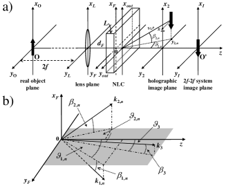
Figure 1: a) Propagation scheme; NLC, nonlinear crystal. b) Interaction inside the crystal, optical axis on the shaded plane.

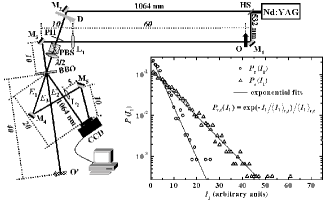
Figure 2: Experimental setup: HS, harmonic separator; D, diffusing plate; M_1-5, mirrors. Lens L₁ images O into O^′ through a $2f-2f$ system. Lens L_1-2, lenses. Distances are in cm. Inset: logarithmic plot of $P_{{\bf r},t}({I}_{1})$.

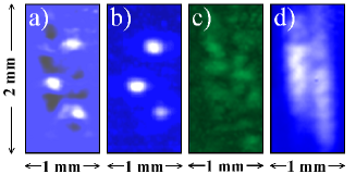
Figure 3: a) Map of $G\left({I}_{1,j},{I}_{2}(x_{2},y_{2})\right)$ evaluated on 1000 shots. b) Plane wave image. Chaotic images: c) single-shot and d) average over 1000 shots.

References

- (1) M. I. Kolobov, Rev. Mod. Phys. 71, 1539-1589 (1999).
- (2) B. E. A. Saleh, A. F. Abbouraddy, A. V. Sergienko, and M. C. Teich, Phys. Rev. A 62, 043816 (2000).
- (3) A. V. Belinskii and D. N. Klyshko, JETP 105, 259-262 (1994).
- (4) P. H. S. Ribeiro, S. Padua, J. C. Machado da Silva and G. A. Barbosa, Phys. Rev. A 49, 4176-4179 (1994).
- (5) D. V. Strekalov, A. V. Sergienko, D. N. Klyshko, and Y. H. Shih, Phys. Rev. Lett. 74, 3600-3603 (1995).
- (6) G. A. Barbosa, Phys. Rev. A 54, 4473-4477 (1994).
- (7) R. S. Bennink, S. J. Bentley, and R. W. Boyd, Phys. Rev. Lett. 89, 113601 (2002).
- (8) R. S. Bennink, S. J. Bentley, and R. W. Boyd, Phys. Rev. Lett. 92, 033601 (2004).
- (9) A. Gatti, E. Brambilla, and L. A. Lugiato, Phys. Rev. Lett. 90, 133603 (2003).
- (10) J. Cheng, and S. Han, Phys. Rev. Lett. 92, 093903 (2004).
- (11) A. Gatti, E. Brambilla, M. Bache, and L. A. Lugiato, Phys. Rev. A. 70, 013802 (2004).
- (12) D. Magatti, F. Ferri, A. Gatti, M. Bache, E. Brambilla, and L. A. Lugiato, arXiv:quant-ph/0408021.
- (13) A. F. Abouraddy, B. E. E. Saleh, A. V. Sergienko, and M. C. Teich, J. Opt. Soc. Am. B19, 1174-1184, (2002).
- (14) T. B. Pittman, Y. H. Shih, D. V. Strekalov, and A. V. Sergienko, Phys. Rev. A 52, R3429-R3429 (1995).
- (15) C. H. Monken, P. H. S. Ribeiro, and S. Padua, Phys. Rev. A 57, 3123-3126 (1998).
- (16) D. P. Caetano, P. H. S. Ribeiro, J. T. C. Pardal, and A. Z. Khoury, Phys. Rev. A 68, 023805 (2003).
- (17) A. Andreoni, M. Bondani, Yu. N. Denisyuk, and M. A. C. Potenza, J. Opt. Soc. Am. B 17, 966-972 (2000).
- (18) M. Bondani and A. Andreoni, Phys. Rev. A 66, 033805 (2002).
- (19) M. Bondani, A. Allevi, A. Brega, E. Puddu and A. Andreoni, J. Opt. Soc. Am. B21, 280-288 (2004).
- (20) M. Bondani, A. Allevi, E. Puddu and A. Andreoni, manuscript in preparation.

References

- (1) M. I. Kolobov, The spatial behavior of nonclassical light, Rev. Mod. Phys. 71, 1571 (1999).
- (2) B. E. A. Saleh, A. F. Abbouraddy, A. V. Sergienko, and M. C. Teich, Duality between partial coherence and partial entanglement, Phys. Rev. A 62, 043816 (2000).
- (3) A. V. Belinskii and D. N. Klyshko, Two-photon optics: diffraction, holography, and transformation of two-dimensional signals, JETP 105, 260 (1994).
- (4) P. H. S. Ribeiro, S. Padua, J. C. Machado da Silva and G. A. Barbosa, Controlling the degree of visibility of Young’s fringes with photon coincidence measurements, Phys. Rev. A 49, 4176 (1994).
- (5) D. V. Strekalov, A. V. Sergienko, D. N. Klyshko, and Y. H. Shih, Observation of two-photon ”ghost” interference and diffraction, Phys. Rev. Lett. 74, 3600 (1995).
- (6) G. A. Barbosa, Quantum images in double-slit experiments with spontaneous down-conversion light, Phys. Rev. A 54, 4473 (1994).
- (7) R. S. Bennink, S. J. Bentley, and R. W. Boyd, ”Two-photon” coincidence imaging with a classical source, Phys. Rev. Lett. 89, 113601 (2002).
- (8) R. S. Bennink, S. J. Bentley, and R. W. Boyd, Quantum and classical coincidence imaging, Phys. Rev. Lett. 92, 033601 (2004).
- (9) A. Gatti, E. Brambilla, and L. A. Lugiato, Entangled imaging and wave-particle duality: from the microscopic to the macroscopic realm, Phys. Rev. Lett. 90, 133603 (2003).
- (10) J. Cheng, and S. Han, Incoherent coincidence imaging and its applicability in X-ray diffraction, Phys. Rev. Lett. 92, 093903-1 (2004).
- (11) A. Gatti, E. Brambilla, M. Bache, and L. A. Lugiato, Correlated imaging, quantum and classical, Phys. Rev. A. 70, 013802 (2004).
- (12) D. Magatti, F. Ferri, A. Gatti, M. Bache, E. Brambilla, and L. A. Lugiato, Experimental evidence of high-resolution ghost imaging and ghost diffraction with classical thermal light, arXiv:quant-ph/0408021.
- (13) T. B. Pittman, Y. H. Shih, D. V. Strekalov, and A. V. Sergienko, Optical imaging by means of two-photon quantum entanglement, Phys. Rev. A 52, R3429 (1995).
- (14) C. H. Monken, P. H. S. Ribeiro, and S. Padua, Transfer of angular spectrum and image formation in spontaneous parametric down-conversion, Phys. Rev. A 57, 3123 (1998).
- (15) D. P. Caetano, P. H. S. Ribeiro, J. T. C. Pardal, and A. Z. Khoury, Quantum image control through polarization entanglement in parametric down-conversion, Phys. Rev. A 68, 023805 (2003).
- (16) A. Andreoni, M. Bondani, Yu. N. Denisyuk, and M. A. C. Potenza, Holographic properties of the second harmonic cross-correlation of object and reference optical wave fields, J. Opt. Soc. Am. B 17, 977 (2000).
- (17) M. Bondani and A. Andreoni, Holographic nature of three-wave mixing, Phys. Rev. A 66, 033805 (2002).
- (18) M. Bondani, A. Allevi, A. Brega, E. Puddu and A. Andreoni, Difference-Frequency-Generated Holograms of 2D-Objects, J. Opt. Soc. Am. B21, 280 (2004).
- (19) M. Bondani, A. Allevi, E. Puddu and A. Andreoni, manuscript in preparation.