Quantum correlations in bound-soliton pairs and trains in fiber lasers

Abstract

Quantum correlations in pairs and arrays (trains) of bound solitons modeled by the complex Ginzburg-Landau equation (CGLE) are calculated numerically, on the basis of linearized equations for quantum fluctuations. We find strong correlations between the bound solitons, even though the system is dissipative. Some degree of the correlation between the photon-number fluctuations of stable bound soliton pairs and trains is attained and saturates after passing a certain distance. The saturation of the photon- number correlations is explained by the action of non- conservative terms in the CGLE. Photon-number-correlated bound soliton trains offer novel possibilities to produce multipartite entangled sources for quantum communication and computation.

Solitons in optical fibers are well known for their remarkable dynamical properties, at both classical and quantum levels. As concerns the latter, the solitons are macroscopic optical fields that exhibit quadrature-field squeezing of quantum fluctuations around the classical core Drummond87 ; Lai89 ; Lai90 , as well as amplitude squeezing Friberg ; RK-fbg , and both intra-pulse and inter-pulse correlations Schmidt00 . Due to the Kerr nonlinearity of the fiber, the quantum fluctuations about the temporal solitons get squeezed during the propagation, i.e., the variance of the perturbed quadrature field operator around the soliton is smaller than in the vacuum state. The nonlinear Schrödinger equation (NLSE) is a commonly adopted model for the description of classical and quantum dynamics in optical fibers. Experimental investigations of quantum properties of temporal solitons have shown remarkable agreement with predictions of the NLSE, provided that loss and higher-order effects are negligible Friberg ; Rosenbluh ; Bergman91 ; Yu01 ; Krylov99 ; Spalter .

In the NLSE, adjacent temporal solitons attract or repel each other, depending on the phase shift between them Agrawal95 . In the cases when the potential interaction force between the solitons can be balanced by additional effects, such as those induced by small loss and gain terms in a perturbed cubic Malomed91 ; Jena or quintic NLSE Akhmediev96 ; Akhmediev97 ; Soto97 ; Seva ; Akhmediev98 [which actually turns the NLSE equation into a complex Ginzburg-Landau equation (CGLE)], or the polarization structure of the optical field, described by the coupled NLSEs Haelterman93 ; Kaup93 ; Malomed98 , bound states of solitons have been predicted. Recently, formation of stable double-, triple-, and multi-soliton bound states (trains, in the latter case) has been observed experimentally in various passively mode-locked fiber-ring laser systems Tang01 ; Seong02 ; Grelu03 , which offers potential applications to optical telecommunications. Formation of “soliton crystals” in nonlinear fiber rings has been predicted too Fedor .

Multiple-pulse generation in the passively mode-lock fiber lasers is quite accurately described by the quintic CGLE (which is written here in a normalized form),

$$iU_{z}+\frac{D}{2}U_{tt}+|U|^{2}U = i\delta U+i\epsilon|U|^{2}U+i\beta U_{tt}$$ (1)

$$+ i\mu|U|^{4}U-v|U|^{4}U,$$

where $U$ is the local amplitude of the electromagnetic wave, $z$ is the propagation distance, $t$ is the retarded time, and $D$ corresponds to anomalous dispersion ($+1$) or normal dispersion ($-1$). Besides the group-velocity dispersion (GVD) and Kerr effect, which are accounted for by conservative terms on the left-hand-side of Eq. (1), the equation also includes the quintic correction to the Kerr effect, through the coefficient $\nu$, and non-conservative terms (the coefficients $\delta$, $\epsilon$, $\mu$, and $\beta$ account for the linear, cubic, and quintic loss or gain, and spectral filtering, respectively).

In quantum-squeezing experiments, additional noises due to the processes other than the GVD and Kerr effect, such as the acoustic- wave Brillouin scattering, are unwanted and suppressed, using stable fiber lasers Yu01 . Accordingly, the non-conservative terms in the CGLE may be superficially considered as detrimental to the observation of quantum fluctuations of fiber solitons. However, an accurate analysis of the quantum fluctuations in the CGLE- based model is necessary, and was missing thus far, to the best of our knowledge.

The objective of the present work is to calculate quantum fluctuations around bound states of solitons in the CGLE by dint of a numerically implemented back-propagation method Lai95 . We find strong quantum-perturbation correlations between the bound solitons, despite the fact the dissipative nature of the model will indeed prevent observation of the squeezing of the quantum fluctuations around the bound solitons in the fiber-ring lasers described by the CGLE. Multimode quantum-correlation spectra of the bound-soliton pairs show patterns significantly different from those for two-soliton configurations in the conservative NLSE. We also find that a similarity in the photon-number correlations between the stable bound-soliton pairs and multi-soliton trains.

Following the known approach to the investigation of bound- soliton states Malomed91 ; Akhmediev96 ; Seva , the corresponding solution to Eq. (1) is sought for in the form

$$U(z,t)=\sum_{j=1}^{N}U_{0}(z,t+\rho_{j})e^{i\theta_{j}},$$

where $U_{0}$ is a single-soliton solution, and $\rho_{j}$ and $\theta_{j}$ are the coordinates separation and phases of the individual solitons. Through the balance between the gain and loss, in- phase and out-of-phase bound-soliton pairs may exist in the anomalous-GVD regime, which is described by Eq. (1). In the case of the normal dispersion, which corresponds to the opposite sign in front of $U_{tt}$ on the left-hand side of Eq. (1), strongly chirped solitary pulses (which differs them from the classical solitons) and their bound states are possible too.

To evaluate the quantum fluctuations around the bound solitons, we replace the classical function $U(z,t)$ in Eq. (1) by the quantum-field operator variable, $\hat{U}(z,t)$, which satisfies the equal-coordinate Bosonic commutation relations. Next we linearize the equation around the classical solution, i.e. $\hat{U}(z,t)=U_{0}+\hat{u}(z,t)$, for a state containing a very large number of photons. Then, the above-mentioned back-propagation method is used to calculate the perturbed quantum fluctuations around the bound-soliton states in the full CGLE model. The linearized equation for the perturbed field operator $\hat{u}(z,t)$ is,

$$\frac{d}{dz}\hat{u}(z,t)={\cal P}_{1}(z,t)\hat{u}(z,t)+{\cal P}_{2}(z,t)\hat{u}^{\dagger}(z,t)+\hat{n}(z,t),$$ (2)

where ${\cal P}_{1}$ and ${\cal P}_{2}$ are two special operators defined as follows,

$${\cal P}_{1}(z,t) = i\frac{D}{2}\frac{\partial^{2}}{\partial t^{2}}+2i|U_{0}|^{2}+\delta+2\epsilon|U_{0}|^{2}+\beta\frac{\partial^{2}}{\partial t^{2}}$$

$$+ 3\mu|U_{0}|^{4}+3i\nu|U_{0}|^{4},$$

$${\cal P}_{2}(z,t) = iU_{0}^{2}+\epsilon U_{0}^{2}+2\mu U_{0}^{3}U_{0}^{\ast}+2i\nu U_{0}^{3}U_{0}^{\ast}.$$

To satisfy the Bosonic communication relations for the perturbed quantum fields $\hat{u}(z,t)$ and $\hat{u}^{\dagger}(z,t)$, we also introduce a zero-mean additional noise operator $\hat{n}(z,t)$ in Eq. (2), with satisfy following commutation relations Lai95 ,

$$[\hat{n}(z,t_{1}) \hat{n}^{\dagger}(z^{\prime},t_{2})]=$$ ,

$$\{-{\cal P}_{1}(z,t_{1})-{\cal P}_{1}^{\ast}(z^{\prime},t_{2})\}\delta(z-z^{\prime})\delta(t_{1}-t_{2}),$$

$$[\hat{n}(z,t_{1}) \hat{n}(z^{\prime},t_{2})]=[\hat{n}^{\dagger}(z,t_{1}),\hat{n}^{\dagger}(z^{\prime},t_{2})]=0.$$ ,

To actually determine the correlation functions of $\hat{n}(z,t)$ and $\hat{n}^{\dagger}(z,t)$, one has to consider its physical origins. In general, $\hat{n}(z,t)=\sum_{i}\hat{n}_{i}(z,t)$, with $\hat{n}_{i}(z,t)$ being the noise operator contributed by the i-th non-conservative term in the equation. The commutation relations of $\hat{n}_{i}(z,t)$ and $\hat{n}_{i}^{\dagger}(z,t)$ are of the same form as in the above equations for $\hat{n}(z,t)$ and $\hat{n}^{\dagger}(z,t)$, except that the differential operators $P_{1}(z,t)$ and $P_{2}(z,t)$ contain only the corresponding non-conservative term. For simplicity, in our calculation we will introduce the following assumptions: $\langle\hat{n}_{i}^{\dagger}(z,t_{1})\hat{n}_{i}(z^{\prime},t_{2})\rangle=0$ for loss terms and $\langle\hat{n}_{i}(z,t_{1})\hat{n}_{i}^{\dagger}(z^{\prime},t_{2})\rangle=0$ for gain terms. With these additional assumptions, the correlation functions for each $\hat{n}_{i}(z,t)$ as well as for the total noise $\hat{n}(z,t)$ can be calculated from their commutation relations. Physically, these assumptions are equivalent to assume the reservoirs corresponding to the loss terms are in the ground state and the population inversions corresponding to the gain terms are in full inversion. The magnitude of the noise level calculated with these assumptions represents the minimum quantum noise that will be introduced with the presence of the considered non-conservative terms. For real systems, the actual introduced noises will be always larger and thus our calculation results here only represent the lower bound limit required by the fundamental quantum mechanics principles.

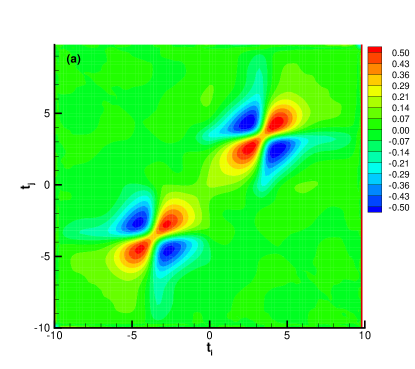
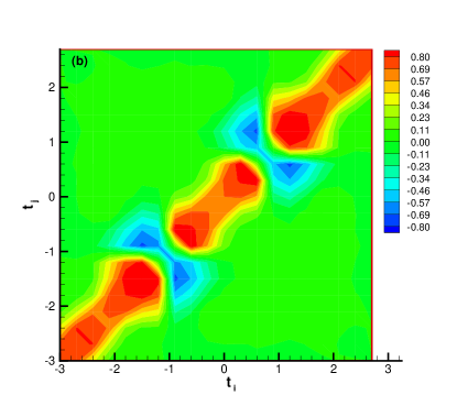
Figure 1: A typical pattern of the time-domain photon-number correlations, $\eta_{ij}$, for an out-of-phase two- soliton state in the cubic NLSE model (a), after $6$ normalized propagation distance; and for an in-phase two- soliton bound state in the CGLE model (b), after $0.5$ normalized propagation distance.

In Fig. 1, we display the comparison of the time-domain photon-number correlations for the two- soliton configuration in the conservative cubic NLSE model (a), and an in- phase two-soliton bound state in the CGLE model (b). The correlation coefficients, $\eta_{ij}$, are defined through the normally-ordered covariance,

$$\eta_{ij}\equiv\frac{\langle:\Delta\hat{n}_{i}\Delta\hat{n}_{j}:\rangle}{\sqrt{\Delta\hat{n}_{i}^{2}\Delta\hat{n}_{j}^{2}}}~{},$$ (3)

where $\Delta\hat{n}_{j}$ is the photon- number fluctuation in the $j$-th slot $\Delta t_{j}$ in the time domain,

$$\Delta\hat{n}_{j}=\int_{\Delta t_{j}}d\,t[U_{0}(z,t)\hat{u}^{{\dagger}}(z,t)+U_{0}^{\ast}(z,t)\hat{u}(z,t)].$$

Here $\hat{u}(z,t)$ and $U_{0}(z,t)$ are the quantum-field perturbation and classical unperturbed solution, as defined above, and the integral is taken over the given time slot. In the NLSE model, there are two isolated patterns for the two- solitons configuration, corresponding to the intra-pulse correlations of individual solitons, see Fig. 1(a). However, it is obvious from Fig. 1(b) that there is a band of strong correlations between the two bound solitons in the quantum CGLE model. This strong-correlation band can be explained by the interplay between the nonlinearity, GVD, gain, and loss in the model. The balance between these features not only supports the classical stable bound state of the soliton, but also causes strong correlations between their quantum fluctuations.

In addition to the time-domain photon-number correlation pattern, we have also calculated a photon-number correlation parameter between the two bound solitons, which is defined as

$$C_{12}=\frac{\langle:\Delta\hat{N}_{1}\Delta\hat{N}_{2}:\rangle}{\sqrt{\langle\Delta\hat{N}_{1}^{2}\rangle\langle\Delta\hat{N}_{2}^{2}\rangle}}.$$

Here, $\Delta\hat{N}_{1,2}$ are perturbations of the photon-number operators of the two solitons, which are numbered (1,2) according to their position in the time domain.

Figure 2 shows the evolution of the photon-number correlation parameter in the two-soliton bound state. Initially, the classical laser statistics (coherent state) is assumed for each soliton, without correlation between them, $C_{12}\approx 0$. In the course of the evolution, the photon-number correlation between the two bound solitons gradually increases to positive values of $C_{12}$, and eventually it saturates about $C_{12}=0.36$. The inter- soliton correlation is induced and supported by the interaction between the solitons. In a conservative system, such as the NLSE model, nearly perfect photon-number correlations can be established if the interaction distance is long enough RK-en04 . In a non-conservative system, such as in the CGLE model, the action of the filtering, linear and nonlinear gain, and losses lead to the saturation of the photon-number correlation parameter. Thus, while the large quantum fluctuations in the output bound- soliton pair will eclipse any squeezing effect, the correlated fluctuations between the bound soliton are predicted to be observable.

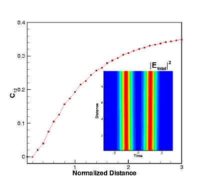
Figure 2: The evolution of the photon-number correlation parameter, $C_{12}$, for two bound in-phase. The computations were carried out for the following values of parameters in the CGLE: $D=1$, $\delta=-0.01$, $\epsilon=1.8$, $\beta=0.5$, $\mu=-0.05$, and $\nu=0$. The inset illustrates the stability of the underlying classical solution for the two- soliton bound state, by means of contour plots.

The approach elaborated here for the study of the quantum-noise correlations between two bound solitons can be easily extended to multi-soliton bound states (soliton trains). Figure 3 shows the photon-number correlation parameters, $C_{ij}$, in a train of four equal-separated in-phase bound solitons. Again, the photon-number fluctuations are initially uncorrelated between the solitons. As could be expected, we find that soliton pairs with equal separations have practically identical correlation coefficients, i.e. , $C_{12}(z)\approx C_{23}(z)\approx C_{34}(z)$, and $C_{13}(z)\approx C_{24}(z)$. Obviously, when the interaction between the soliton trains is stronger, as the separation between them is smaller, the values of the correlation parameter are larger. Note that the correlation coefficient for the most separated pair in the train, $C_{14}$, grows very slowly with $z$. Eventually, all of the curves of $C_{ij}(z)$ saturate due to the dissipative effects in the CGLE model.

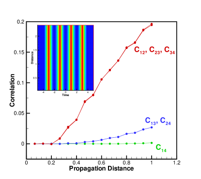
Figure 3: The evolution of the photon-number correlation parameters, $C_{ij}$, for a bound complex (train) of four in-phase solitons in the CGLE model. The soliton’s number ($1,2,3,4$) runs from left to right. Parameters are the same as in the case shown in Fig. (2). The inset demonstrates the stability of the underlying classical solution for the four-soliton train.

In conclusion, in this paper we have extended the concept of quantum fluctuation around classical optical solitons to the non-conservative model based on the CGLE (complex Ginzburg-Landau equation) with the cubic-quintic nonlinearity. Applying the known back-propagation method to the linearized equations that govern the evolution of the fluctuations, we have numerically calculated the photon-number correlations and the effective correlation coefficient for pairs of bound solitons, as well as for multi-soliton bound complexes (trains). We have demonstrated that, unlike the two-soliton configuration in the conservative NLSE model, there is a band of strong quantum correlation in the bound-soliton pair. While the dissipative effects in the CGLE model will totally suppress the generation of squeezed states from bound solitons, as one might expect, there still exists a certain degree of correlations between photon-number fluctuations around the stable bound-soliton pairs and trains. Recently, experimental progress in the study of various quantum properties of solitons in optical fibers has been reported Silberhorn01 ; Silberhorn02 ; Glockl03 ; Konig02 , which opens the way to observe effects predicted here. Besides that, the photon- number-correlated soliton pairs and trains, predicted in this work, may offer new possibilities to generate multipartite entangled sources for applications to quantum communications and computation.

References

- (1) P. D. Drummond and S. J. Carter, J. Opt. Soc. Am. B 4, 1565 (1987).
- (2) Y. Lai and H. A. Haus, Phys. Rev. A. 40, 844 (1989); ibid 40, 854 (1989).
- (3) Y. Lai and H. A. Haus, Phys. Rev. A 42, 2925 (1990).
- (4) S. R. Friberg, S. Machida, M. J. Werner, A. Levanon, and T. Mukai, Phys. Rev. Lett. 77, 3775 (1996).
- (5) R.-K. Lee and Y. Lai, Phys. Rev. A 69, 021801(R) (2004).
- (6) E. Schmidt, L. Knöll, D.-G. Welsch, M. Zielonka, F. König, and A. Sizmann, Phys. Rev. Lett. 85, 3801 (2000).
- (7) M. Rosenbluh and R. M. Shelby, Phys. Rev. Lett. 66, 153 (1991).
- (8) K. Bergman and H. A. Haus, Opt. Lett. 16, 663 (1991).
- (9) C. X. Yu, H. A. Haus, and E. P. Ippen, Opt. Lett. 26, 669 (2001).
- (10) D. Krylov, K. Bergman, and Y. Lai, Opt. Lett. 24, 774 (1999).
- (11) S. Spälter, N. Korolkova, F. König, A. Sizmann, and G. Leuchs, Phys. Rev. Lett. 81, 786 (1998).
- (12) G. P. Agrawal, Nonlinear Fiber Optics, (Academic, San Diego, 1995); Yu. S. Kivshar and G. P. Agrawal. Optical Solitons: From Fibers to Photonic Crystals (Academic, San Diego, 2003).
- (13) B. A. Malomed, Phys. Rev. A44, 6954, (1991).
- (14) I. M. Uzunov, R. Muschall, M. Gölles, F. Lederer, and S. Wabnitz, Opt. Commun. 118, 577 (1995).
- (15) N. N. Akhmediev, V. V. Afanasjev, and J. M. Soto-Crespo, Phys. Rev. E53, 1190 (1996).
- (16) N. N. Akhmediev, A. Ankiewicz, and J. M. Soto-Crespo, Phys. Rev. Lett. 79, 4047 (1997).
- (17) J. M. Soto-Crespo, N. N. Akhmediev, V. V. Afanasjev, and S. Wabnitz, Phys. Rev. E55, 4783 (1997).
- (18) V. V. Afanasjev, B. A. Malomed, and P. L. Chu, Phys. Rev. E 56, 6020 (1997).
- (19) N. N. Akhmediev, A. Ankiewicz, and J. M. Soto-Crespo, J. Opt. Soc. Am. B15, 515 (1998).
- (20) M. Haelterman, A. P. Sheppard, and A. W. Snyder, Opt. Lett. 18, 1406 (1993).
- (21) D. J. Kaup, B. A. Malomed, and R. S. Tasgal, Phys. Rev. E48, 3049, (1993).
- (22) B. A. Malomed and R. S. Tasgal, Phys. Rev. E58, 2564 (1998).
- (23) D. Y. Tang, W. S. Man, H. Y. Tam, and P. D. Drummond, Phys. Rev. A64, 033814 (2001).
- (24) N. H. Seong and Dug Y. Kim, Opt. Lett. 27, 1321 (2002).
- (25) P. Grelu, F. Belhache, F. Gutty, and J. M. Soto-Crespo, J. Opt. Soc. Am. B20, 863 (2003).
- (26) G. Steinmeyer and F. Mitschke, Appl. Phys. B 62, 367 (1996); B. A. Malomed, A. Schwache, and F. Mitschke, Fiber Int. Opt. 17, 267 (1998).
- (27) Y. Lai and S.-S. Yu, Phys. Rev. A51, 817 (1995).
- (28) R.-K. Lee, Y. Lai, and B. A. Malomed, quant-ph/0405138.
- (29) Ch. Silberhorn, P. K. Lam, O. Weiss, F. König, N. Korolkova, and G. Leuchs, Phys. Rev. Lett. 86, 4267 (2001).
- (30) Ch. Silberhorn, N. Korolkova, and G. Leuchs, Phys. Rev. Lett. 88, 167902 (2002).
- (31) O. Glöckl, S. Lorenz, C. Marquardt, J. Heersink, M. Brownnutt, C. Silberhorn, Q. Pan, P. van Loock, N. Korolkova, and G. Leuchs, Phys. Rev. A68, 012319 (2003).
- (32) F. König, M. A. Zielonka, and A. Sizmann, Phys. Rev. A66, 013812 (2002).