NMR Quantum Information Processing

Abstract

Nuclear Magnetic Resonance (NMR) has provided a valuable experimental testbed for quantum information processing (QIP). Here, we briefly review the use of nuclear spins as qubits, and discuss the current status of NMR-QIP. Advances in the techniques available for control are described along with the various implementations of quantum algorithms and quantum simulations that have been performed using NMR. The recent application of NMR control techniques to other quantum computing systems are reviewed before concluding with a description of the efforts currently underway to transition to solid state NMR systems that hold promise for scalable architectures.

I Introduction

Nuclear spins feature prominently in most condensed matter proposals for quantum computing c1 ; c2 ; c3 ; c4 ; c5 ; c6 ; c7 ; c8 ; c9 ; c10 , either directly being used as computational or storage qubits, or being important sources of decoherence. Fortunately, the coherent control of nuclear spins has a long and successful history driven in large part by the development of nuclear magnetic resonance (NMR) techniques in biology, chemistry, physics, and medicine c11 ; c12 . The central feature of NMR that makes it amenable to quantum information processing (QIP) experiments is that, in general, the spin degrees of freedom are separable from the other degrees of freedom in the systems studied, both in the liquid and solid state. We can therefore describe the Hamiltonian of the spin system quite accurately; there is an extensive literature on methods to control nuclear spins, and the hardware to implement such control is quite precise.

This readily accessible control of nuclear spins has led to liquid state NMR being used as a testbed for QIP, as well as to preliminary studies of potentially scalable approaches to QIP based on extensions of solid state NMR. The liquid state NMR QIP testbed, although it is not scalable, has permitted studies of control and QIP in Hilbert spaces larger than are presently available with other modalities, and has helped to provide concrete examples of QIP. Here we review what has been learnt in these initial studies and how they can be extended to the solid state where scalable implementations of QIP appear to be possible.

The DiVincenzo criteria DiVincenzo (2000) for quantum computation provide a natural starting place to understand why NMR is such a good testbed for QIP, and in particular, for implementing quantum algorithms using liquid state NMR techniques. These criteria concern (1) the qubits, (2) the initial state preparation, (3) the coherence times, (4) the logic gates, and (5) the readout mechanism.

I.1 Quantum Bits

Protons and neutrons are elementary particles which carry spin-$1/2$, meaning that in a magnetic field $\vec{B}$, they have energy $-\vec{\mu}\cdot\vec{B}$, where the magnetic moment $\vec{\mu}=\mu_{N}\vec{I}$ ($\vec{I}$ is the spin operator) is quantized into two energy states, $|\downarrow\rangle$ and $|\uparrow\rangle$ . These states have an energy scale determined by the nuclear Bohr magneton $\mu_{N}=eh/2m_{N}\approx 5.1\times 10^{-27}$ A$/$m² (Table 1). Since spin is inherently a discrete quantum property which exists inside a finite Hilbert space, spin-$1/2$ systems are excellent quantum bits.

1H	19F	31P	13C	29Si	15N
$500$ MHz	$470$ MHz	$202$ MHz	$125$ MHz	$99$ MHz	$50$ MHz

Table 1: Atoms with spin-1/2 nuclei typically used in NMR, and their energy scales, expressed as a resonance frequency. Frequencies are given for $|\vec{B}|\sim 11.74$ Tesla.

Nuclear spins used in NMR QIP are typically the spin-1/2 nuclei of ¹H, ¹³C, ¹⁹F, ¹⁵N, ³¹P, or ²⁹Si atoms, but higher order spins such as spin-$3/2$ and $5/2$ have also been experimentally investigated. In liquid-state NMR, these atoms are parts of molecules dissolved in a solvent, such that the system is typically extremely well approximated as being $O(10^{18})$ independent molecules. Each molecule is an $N$-spin system, with $N$ magnetically distinct nuclei. Typically, this molecule sits in a strong, static magnetic field, $B_{0}$, oriented along the $\hat{z}$ axis, such that the $N$ spins precess about $\hat{z}$. The spins interact with each other indirectly via inter-atomic electrons sharing a Fermi contact interaction with two (or more) nuclei. The connectivity of the chemical bonds thus determines which nuclei interact.

Since the energy scale of the interactions is weak compared with typical values of $\mu_{N}|\vec{B}|$, qubits in molecules can be independently manipulated, and provide a natural tensor product Hilbert space structure. This structure is essential for quantum computing, and in particular, system scalability.

I.2 Initial state preparation

The energy scale of a nuclear spin in typical magnetic fields is much smaller than that of room temperature fluctuations. As seen in Table 1, at $11.74$ T the proton has an NMR resonance frequency of $500$ MHz, whereas room temperature thermal fluctuations are $k_{B}T\approx 25$ meV $\approx 6$ THz, about $10^{4}$ times larger. As the Boltzmann distribution governs the thermal equilibrium state of the spins

$$\rho=\frac{\exp\left[\rule{0.0pt}{10.33327pt}{-\frac{\mu_{N}|\vec{B}|}{k_{B}T}}\right]}{\cal Z}\,,$$ (1)

where ${\cal Z}$ is the partition function normalization factor, $\rho\approx$ 1 for $k_{B}T\gg\mu_{N}|\vec{B}|$. Thus, the room temperature thermal equilibrium state is a very highly random distribution, with spins being in their $|\downarrow\rangle$ and $|\uparrow\rangle$ states with nearly equal probability.

Such a highly mixed state is not ordinarily suitable for quantum computation, which ideally works with a system initialized to a fiducial state such as $|00\cdots 0\rangle$. It was the discovery of a set of procedures to circumvent this limitation, which made NMR quantum information processing feasible and interesting Cory et al. (1997); Gershenfeld and Chuang (1997). The essential observation is that a $computational$ procedure can be applied to $\rho$, such that the only observed signal comes from the net excess population in the $|00\cdots 0\rangle$ state of the thermal ensemble. One class of such techniques averages away the signal from all other states. This averaging can be performed sequentially in time using sequences of pulses which symmetrically permute undesired states, spatially using magnetic field gradients which prepare spins differently in different parts of a single sample, or by selecting a special subset of spins depending on the logical state ($|0\rangle$ or $|1\rangle$) of the unselected spins. These techniques, known as temporal, spatial, and logical labeling, do not scale well, and only create a signal strength which decreases exponentially with the number of qubits realized Warren (1997).

Another class of techniques is based on efficient compression Schulman and Vazirani (1998), and in contrast, the signal strength obtained is constant with increasing number of qubits realized. Indeed, only $O({\rm poly}(n))$ space and time resources are needed to initialize $O(n)$ spins using this method, which has now been experimentally demonstrated Chang et al. (2001), but there is a constant overhead factor which prevents it from being practical until $n$ is large, or the initial temperature of the spins can be brought lower by several orders of magnitude.

I.3 Coherence times

Nuclear spins couple very weakly with the external world, primarily due to their small magnetic moment, and the weakness of long-range magnetic forces. Thus, typical nuclei in liquid-state molecules may have a $T_{1}$ timescale for energy relaxation of between $1$ and $30$ seconds, and a $T_{2}$ timescale for phase randomization of between $0.1$ and $10$ seconds. Decoherence may occur due to the presence of quadrupolar nuclei such as ³⁵Cl and ²D, chemical shift anisotropies, fluctuating dipolar interactions, and other higher order effects. Though the coherence lifetimes are long, the number of gates that can be implemented is limited by the relatively weak strength of the qubit-qubit couplings (typically a few hundred Hz at most).

I.4 Logic gates

In order to perform arbitrary quantum computations only a finite set of logic gates is required, similar to arbitrary classical computations. One such set consists of arbitrary single qubit rotations and the two-qubit controlled-not gate. We describe how each of these is implemented.

The Hamiltonian describing a 2-spin system in an external field $B_{0}\hat{z}$ is (setting $\hbar=1$)

$${\cal H}=\omega_{A}I_{zA}+\omega_{B}I_{zB}+{\cal H}_{A,B}\;.$$ (2)

Here, $I_{z}$ is the spin angular momentum operator in the $\hat{z}$ direction, and $\omega_{i}=-\gamma_{i}(1-\alpha_{i})B_{0}$, where $\gamma_{i}$ is the gyromagnetic ratio for spin $i$, which depends on the nuclear species, $\alpha_{i}$ is the shielding constant, and ${\cal H}_{A,B}$ is the spin-spin coupling. The shielding constant depends on the local chemical environment of the nuclei, which shields the local magnetic field, resulting in a shift in frequency by an amount known as the chemical shift such that spins of the same type (e.g. protons) can have different resonance frequencies. That spins have different resonance frequencies is an important requirement because it permits frequency-dependent addressing of single qubits.

Spins are manipulated by applying a much smaller radio-frequency (RF) field, $B_{1}$, in the $\hat{x}$-$\hat{y}$ plane to excite the spins at their resonance frequencies $\omega_{i}$. In the rotating frame, to good approximation, the spin evolves under an effective field $\vec{B}=B_{1}\cos(\phi)\hat{x}+B_{1}\sin(\phi)\hat{y}$ (where $\phi$ is the RF phase). The rotation angle and axis (in the transverse plane) can be controlled by varying $\phi$, the magnitude of $B_{1}$ and the duration of the RF. Since it is possible to generate arbitrary rotations about the $\hat{z}$-axis using combinations of rotations about the $\hat{x}$ and $\hat{y}$-axis, it is possible to implement arbitrary single-qubit rotations using RF pulses.

Two-qubit gates, such as the controlled-not gate require spin-spin interactions. These occur through two dominant mechanisms; direct dipolar coupling, and indirect through-bond interactions. The dipolar coupling between two spins is described by an interaction Hamiltonian of the form

$${\cal H}_{A,B}^{D}=\frac{\gamma_{A}\gamma_{B}}{r^{3}}\left(\vec{I}_{A}\cdot\vec{I}_{B}-3(\vec{I}_{A}\cdot\hat{n})(\vec{I}_{B}\cdot\hat{n})\right),$$ (3)

where $\hat{n}$ is the unit vector in the direction joining the two nuclei, and $\vec{I}$ is the magnetic moment vector. While dipolar interactions are rapidly averaged away in a liquid, they play a significant role in liquid crystal Yannoni et al. (1999); Marjanska et al. (2000) and solid state NMR QIP experiments. Through-bond electronic interactions are an indirect interaction, also known simply as the scalar-coupling, and take on the form

$${\cal H}_{A,B}^{J}=2\pi J\vec{I}_{A}\cdot\vec{I}_{B}=2\pi JI_{zA}I_{zB}+\pi J\left(I_{A+}I_{B-}+I_{A-}I_{B+}\right),$$ (4)

where $J$ is the scalar coupling constant. This interaction is often resolved in liquids. For heteronuclear species (such that the matrix element of the $I_{A+}I_{B-}+I_{A-}I_{B+}$ term is small, when $2\pi J\ll\omega_{A}-\omega_{B}$), the scalar coupling reduces to

$${\cal H}_{A,B}^{J}\approx 2\pi JI_{zA}I_{zB}.$$ (5)

Multiple-qubit interactions, such as the controlled-not (cnot) operation, may be performed by inserting waiting periods between pulses so that J-coupled evolution can occur. For the J-coupled two-spin system, a cnot can be implemented as a controlled phase shift preceded and followed by rotations, given by the sequence ${\cal C}_{AB}=R_{yA}(270=-90)R_{zB}R_{zA}(-90)R_{zAB}(180)R_{yA}(90)$. This is shown schematically in Fig. 1.

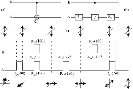
Figure 1: (a) A controlled–NOT gate acting on two qubits, (b) the controlled–NOT gates implemented by a controlled phase shift gate (specified by a unitary matrix with diagonal elements $\{1,1,1,-1\}$) preceded and followed by $\pi/2$ rotations, and (c) the pulse sequence and spin orientations corresponding to the components in (b). Note that, unlike a conventional NMR selective population transfer sequence, extra refocusing is required to preserve the Bell basis exchange symmetry between $A$ and $B$. The $\hat{z}$ rotations are implemented via $\hat{x}$ and $\hat{y}$-rotations, which are not explicitly shown.

In summary, one and two-qubit gates are implemented by applying a sequence of RF pulses interlaced with waiting periods. In this sense, it is perhaps interesting to note that the sequence of elementary instructions (pulses and delay times) are the machine language of the NMR quantum information processor.

I.5 Readout mechanism

Readout of the quantum state in NMR QIP is not the usual ideal projective von Neumann measurement. Instead, the system is continually read out by the weak coupling of the magnetic dipole moments to an external pickup coil, across the ends of which a voltage is produced by Faraday induction. This coil is usually the same coil as that used to produce the strong RF pulses which control the spins, and thus it only detects magnetization in the $\hat{x}-\hat{y}$ plane. The induced voltage, known as the free induction decay, may be expressed as

$$V(t)=-2V_{0}\mbox{\rm tr}\,\left[\rule{0.0pt}{10.33327pt}{e^{-i{\cal H}t}\rho e^{i{\cal H}t}(iI_{x}^{k}+I_{y}^{k})}\right]\,,$$ (6)

where $\cal{H}$ is the Hamiltonian for the spin system, $I_{x}^{k}$ and $I_{y}^{k}$ operate only on the $k^{th}$ spin, and $V_{0}$ is a constant factor dependent on coil geometry, quality factor, and maximum magnetic flux from the sample volume.

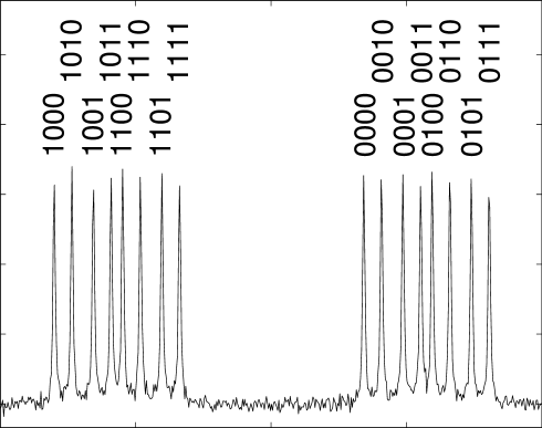
Figure 2: Thermal equilibrium spectrum of a $5$ spin molecule. Each peak corresponds to a certain logical state of the remaining four spins, which is indicated by the binary numbers. The real part of the spectrum is shown, in arbitrary units. Frequencies are given with respect to $\omega_{i}/2\pi$, in Hertz Vandersypen et al. (2000a).

The Fourier transform of $V(t)$ is the NMR spectrum as shown in Fig. 2 for example. When properly calibrated, the NMR spectrum immediately reveals the logical state of qubits which are either $|0\rangle$ or $|1\rangle$. Specifically, for example, if the initial state of a two-spin ¹H-¹³C system is described by a diagonal density matrix,

$$\rho=\left[\begin{array}[]{cccc}a&0&0&0\\ 0&b&0&0\\ 0&0&c&0\\ 0&0&0&d\end{array}\right]$$ (7)

(where the states are $00$, $01$, $10$, and $11$, with proton on left and carbon on right and $a$, $b$, $c$, and $d$ denote the occupation probabilities) then after a $R_{x}(\pi/2)$ readout pulse, the integrals of the two proton peaks (in the proton frequency spectrum) are given by $a-c$ and $b-d$, and the integrals of the two carbon peaks are given by $a-b$ and $c-d$. Both the proton and carbon spectra contain two peaks because of the J-coupling interaction during the measurement period.

One important issue in the readout of QIP results from NMR arises because the system is an ensemble, rather than a single $N$-spin molecule. The problem is that the output of a typical quantum algorithm is a random number, whose distribution gives information which allows the problem to be solved. However, the average value of the random variable would give no relevant information, and this would be the output if the quantum algorithm were executed without modification on an NMR quantum computer.

This problem may be resolved Gershenfeld and Chuang (1997) by appending an additional computational step to the quantum algorithm to eliminate or reduce the randomness of its output. For example, the output of Shor’s algorithm is a random rational number $c/r$, from which classical post-processing is usually employed to determine a number $r$, which is the period of the modular exponentiation function under examination. However, the post-processing can just as well be performed on the quantum computer itself, such that $r$ is determined on each molecule separately. From $r$, the desired prime factors can also be found, and tested; only when successful does a molecule announce an answer, so that the ensemble average reveals the factors. Similar modifications can be made to enable proper functioning of all known exponentially fast quantum algorithms Deutsch and Jozsa (1992); Simon (1994); Kitaev (1995) on an NMR quantum computer.

II Quantum Control

Implementing an algorithm on a quantum computer requires performing both unitary transformations and measurements. Errors in the control and the presence of noise can severely compromise the accuracy with which a unitary transform can be implemented. Quantum control techniques are used to maximize the accuracy with which such operations can be performed, given some model for the system’s dynamics. NMR has provided valuable insight into the design of schemes to control quantum systems, as the task of applying pulse sequences to perform operations that are selective, and also robust against experimental imperfections, has been the subject of extensive studies Jones (2003); c14 . A single, isolated quantum system will evolve unitarily under the Hamiltonian of the system. In an ensemble measurement (whether in space or time), an isolated system can also appear to undergo non-unitary dynamics, called incoherent evolution, due to a distribution of fields over the ensemble c15 ; c16 . An open quantum system, interacting with an environment, will decohere if these interactions are not controlled. The study of quantum control using NMR can therefore be separated into three different subsections:

• Coherent control: how can one design RF control schemes to implement the correct unitary dynamics for a single, isolated quantum system ?

• Incoherent noise: how can coherent control be extended to an ensemble, given that the system Hamiltonian will vary across the ensemble ?

• Decoherent noise: how can one achieve the desired control, when coupling to the environment is taken into account ?

II.0.1 Coherent control

The density matrix of a closed system evolves according to the Liouville–Von Neumann equation of motion:

$$\frac{d\rho}{dt}=-i\left[\cal{H}_{\mathrm{int}}+\cal{H}_{\mathrm{ext}},\rho\right]$$ (8)

where ${\cal H}_{\mathrm{int}}$ is the internal Hamiltonian of the system of qubits, and ${\cal H}_{\mathrm{ext}}$ the externally applied control fields. More specifically, extending Eqs. [2] and [4], the internal Hamiltonian for a system of $N$ spin- 1/2 nuclei in a large external magnetic field $B_{0}$ is :

$${\cal H}_{\mathrm{int}}=\sum_{k=1}^{N}-\gamma_{k}(1-\alpha_{k})B_{0}(r)I_{z}^{k}+2\pi\sum_{j>k}^{N}\sum_{k=1}^{N}J_{kj}I^{k}\cdot I^{j}\;\;$$ (9)

where $-\gamma(1-\alpha_{k})B_{0}$(r) is the chemical shift of the $k^{th}$ spin. The corresponding experimentally-controlled RF Hamiltonian is :

$${\cal H}_{\mathrm{ext}}=\sum_{k=1}^{N}-\gamma_{k}f(r)B_{RF}(t)e^{-i\phi(t)I_{z}^{k}}I_{x}^{k}e^{i\phi(t)I_{z}^{k}}$$ (10)

where the time-dependent functions $B_{RF}(t)$ and $\phi(t)$ specify the applied RF control field, while $f(r)$ reflects the distribution of RF field strengths over the sample. The spatial variation of the static and RF magnetic fields leads to incoherence c15 . We will return to this in the next section.

If the total Hamiltonian is time-independent, possibly through transformation into a suitable interaction frame, the equation of motion can be integrated easily and yields a unitary evolution of the density matrix $\rho(t)=U(t)\rho(0)U^{{\dagger}}(t)$. Given an internal Hamiltonian and some control resources, how can we implement a given propagator or prepare a given state? In QIP, it is necessary to implement the correct propagator, which requires designing gates that perform the desired operation regardless of the input state. We will therefore focus our discussion on NMR control techniques that are universal, i.e. whose performance is essentially independent of the input state, although sequences whose performances are state dependent can also be useful for initialization purposes. Average Hamiltonian theory is a powerful tool for coherent control that was initially developed for NMR c17 . Waugh and Harberlen have provided a theoretical framework to implement a desired effective Hamiltonian evolution of a spin system over some period of time. Such a tool fits well into the context of QIP since it aims to implement the correct propagator over the system Hilbert space while refocusing undesired qubit-qubit interactions. The basic idea is to apply a cyclic train of pulses $P=\{P_{j}\}_{j=1}^{M}$ with $\prod P_{j}=$ 1 to the system which, in its simplest form, are assumed to be infinitely short and equally spaced by $\Delta t>0$. The net controlled evolution over the period $T=M\Delta t$ can then be expressed as

$$e^{-i\bar{H}T}=\prod_{k=0}^{M}e^{-iH_{k}\Delta t}$$ (11)

where the ”toggling-frame” Hamiltonians $H_{k}=U_{k}^{{\dagger}}H_{k}U_{k}$ are expressed in terms of the composite pulses $U_{k}=\prod_{j=1}^{k}P_{j},k=1,\ldots,M,U_{0}=$1. Any average Hamiltonian (up to a scalar multiple) can be implemented in NMR systems of distinguishable spins c18 . This work has been extended to correct for some experimental imperfections or uncertainties primarily using symmetry arguments. Composite pulses have also been used to design robust control sequences as they can be designed to be self-compensating for small experimental errors Jones (2003); c14 ; c19 ; c20 ; c21 ; c22 ; c23 ; c24 .

Strong modulation of the spin system currently represents the state of the art in performing selective, controlled operations in large Hilbert spaces (up to 10 qubits). Strong modulation of the spins permits accurate selective rotations while refocusing the internal Hamiltonian during the RF irradiation of the spins c25 . Figure 3 shows the dependence of the fidelities achievable on the available control resources, using this technique c15 . These are simulation results, assuming only unitary dynamics. The fidelities are seen to improve both with improved distinguishability of the spins (higher field strengths), and stronger modulation (increased RF power). The drawback of this technique is that it is not scalable, as the time necessary to find the numerical solutions grows exponentially with the number of qubits (see Vandersypen and Chuang (2004) for a review of other techniques). An alternative, scalable approach that relies on optimization over single and pairs of nuclei has been described Knill et al. (2000), though it does not appear to work as well.

Finally, there is a growing body of work in the area of optimal control theory for quantum systems c27 ; c28 ; c29 , which has also used NMR as an experimental testbed. It is foreseeable that it might be possible to combine the ideas presented in these studies with strong modulation and pulse-shaping techniques to design optimal control sequences, given some knowledge about the system decoherence and the control parameters.

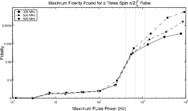
Figure 3: Maximum fidelity achievable versus external magnetic field strengths and maximum radio-frequency power available for strongly modulating pulses. The frequencies shown are the proton Larmor frequencies at different magnetic fields (300 MHz $\equiv$ 7 T, 500 MHz $\equiv$ 11.7 T, 800 MHz $\equiv$ 18.8 T).

II.0.2 Incoherent noise

Incoherent noise arises from a spatial or temporal distribution of experimental parameters in an ensemble measurement c15 . It is manifested in NMR in the spatial dependence of the Hamiltonian ${\cal H}$. The density matrix at a given location in the sample still obeys the Liouville-Von Neumann equation where the internal and external Hamiltonian are now spatially dependent. Since it is the spatially averaged density matrix that is measured, the apparent evolution of the ensemble system is non-unitary and yields the following operator sum representation c30 of the superoperator

$$\rho(t)=\sum_{i}p_{i}U_{i}(t)\rho(0)U_{i}^{{\dagger}}(t)$$ (12)

where $U_{i}$ is a unitary operator and $p_{i}$ represents the fraction of spins that experience a given $U_{i}$ ($\sum_{i}p_{i}=1$). This incoherent evolution can be counteracted using a different set of techniques than those used to deal with the decoherent errors to be discussed in the next section.

Hahn’s pioneering work showed that inhomogeneities in the Hamiltonian could be refocused during an experiment if an external control Hamiltonian orthogonal to the inhomogeneous Hamiltonian was available c32 (see Figure 4). In the case of an inhomogeneous but static Hamiltonian, the correlation time of the noise is infinite. This work was extended by Carr and Purcell to counteract long, but not infinite, correlation time noise fluctuations due to molecular diffusion c31 . Composite pulse sequences have also been used to counteract the effects of incoherent processes c19 ; c20 ; c21 ; c22 ; c23 ; c24 ; c33 ; c34 , but often assume specific input states, or still need to be proven effective over the full Hilbert space of multi-qubit systems. Spin decoupling fits into a similar framework, and provides a means of modulating the system in order to average out unwanted interactions with the environment c35 . It has inspired coherent approaches to other control problems for error correction purposes c36 ; c37 ; c38 .

The use of strongly modulating pulses has been extended to incorporate incoherent effects, considering local unitary dynamics over the ensemble c15 . A priori knowledge of the inhomogeneity of the external Hamiltonian was used to find robust pulse sequences yielding a higher fidelity operation over the ensemble. This knowledge was easily obtained by spectroscopic NMR techniques. Though this work focused on counteracting the main source of incoherent errors in an NMR experiment, i.e. RF inhomogeneity, it could easily be extended to compensate for experimental uncertainties such as the phase noise of the RF irradiation or static $B_{0}$ field inhomogeneities.

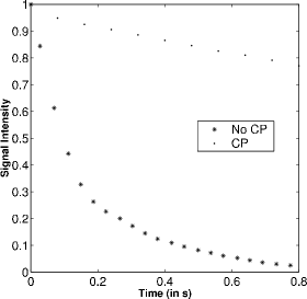
Figure 4: Decay of the transverse magnetization of a nuclear spin in a liquid state sample with large $B_{0}$ field inhomogeneities both with and without a Carr-Purcell (CP) sequence.

II.0.3 Decoherent noise

If the coupling between the system and the environment is weak enough and the correlation time of the noise is short, the evolution of the system is Markovian and obeys the following master equation:

$$\frac{d|\rho(r)\rangle}{dt}=-\left(i\hat{H}(r)+\Gamma\right)|\rho(r)\rangle$$ (13)

where $\Gamma$ is the Liouville space relaxation superoperator c12 . This equation yields a non-unitary evolution of the density matrix so that pure states can evolve into mixed states. To understand and test models of decoherence, methods based on quantum process tomography (QPT) were developed to measure $\Gamma$ c39 ; c40 , so that the dynamics of the system could be simulated more accurately. The full model of the system including coherent, incoherent and decoherent dynamics, has been tested extensively with a three qubit QPT of the Quantum Fourier Transform superoperator c41 . When knowledge about the noise operators is available, quantum error correction (QEC) schemes can in principle be designed to allow quantum computing in the presence of imperfect control. NMR has primarily been used to test the ideas of quantum error correction (QEC) c42 ; c43 ; c44 and of fault-tolerant quantum computations c45 . Experiments were carried out to investigate different QEC scenarios c46 ; c47 ; c48 ; c49 ; c50 ; c51 , in addition to encoded operations acting on logical qubits c52 . Schemes to implement logical encoded quantum operations while remaining in a protected subspace have also been investigated c48 for a simple system made of two physical qubits and are still being studied for larger systems.

III Quantum Algorithms

Many quantum algorithms have now been implemented using liquid-state NMR techniques. The first quantum algorithms implemented with NMR were Grover’s algorithm Chuang et al. (1998a); Jones et al. (1998) and the Deutsch-Jozsa algorithm Chuang et al. (1998b); Jones and Mosca (1998) for two qubits. The quantum counting algorithm was implemented soon afterwards using two-qubits Jones and Mosca (1999). A variety of implementations of Grover’s algorithm and the Deutsch-Jozsa algorithm have subsequently been performed. The two-qubit Grover search was re-implemented using a subsystem of a three qubit system Vandersypen et al. (1999), demonstrating state preparation using logical labeling. A three qubit Grover search has been implemented, in which $28$ Grover iterations were performed, involving $280$ two-qubit gates Vandersypen et al. (2000b). A three-qubit Deutsch-Jozsa algorithm using transition selective pulses Linden et al. (1998), another more advanced version using swap gates to avoid small couplings Collins et al. (2000), and yet another implementation without swap gates Kim et al. (2000). A subset of a five-qubit Deutsch-Jozsa algorithm has also been implemented Marx et al. (2000).

The implementation of quantum algorithms reached a new level with the full implementation of a Shor-type algorithm using five qubits Vandersypen et al. (2000a). This work involved the use of exponentiated permutations, combined with the quantum Fourier transform, which had been previously been implemented Weinstein et al. (2001).

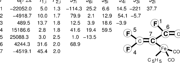
Figure 5: The seven spin molecule used in the quantum factoring NMR experiment, showing its J-coupling constants, $T_{1}$ and $T_{2}$ relaxation times (in seconds), and chemical shifts (in Hertz) at $11.74$ Tesla.

The most complex quantum algorithm realized to-date is the demonstration of Shor’s algorithm using liquid-state NMR QIP methods: In this work Vandersypen et al. (2001), a seven-qubit molecular system was used to factor the number $15$ into its prime factors. This molecule, shown in Fig. 5, was specially chemically synthesized to give resolvable fluorine spectra, in which the two ¹³C nuclei, and the five ¹⁹F nuclei, could each be addressed independently because of the spread of their resonant frequencies. The NMR spectra of this molecule are quite remarkable; for example, the thermal spectrum of ¹⁹F spin number 1 shows 64 lines, corresponding to the random states of the other 6 spins (Fig. 6). Several hundred pulses were applied, with a wide variety of phases, and shapes, at seven different frequencies, in this demonstration of the factoring algorithm (Fig. 7). A comparison of the experimental results with numerical simulations suggests that decoherence was the major source of error in the experiment rather than errors in the unitary control, which is remarkable considering the number of pulses applied.

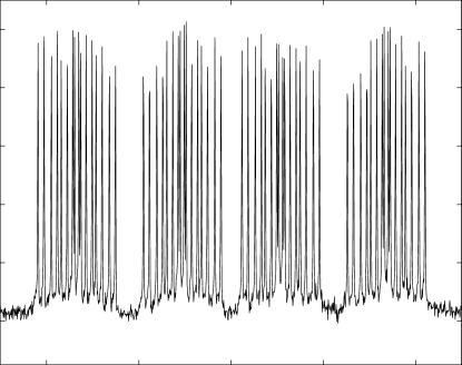
Figure 6: Experimentally measured thermal equilibrium spectra of the NMR spectrum of fluorine atom number 1, in the molecule of Fig. 5. The real part of the spectrum is shown, in arbitrary units. Frequencies are given with respect to $\omega_{i}/2\pi$, in Hertz.

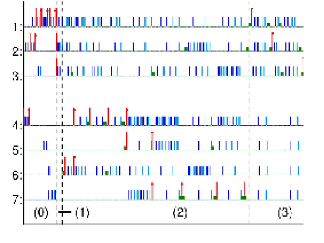
Figure 7: Pulse sequence for implementing Shor’s algorithm to factor $N=15$ (for case $a=7$), using seven qubits. The four steps $0$ through $3$ correspond to different steps in Shor’s algorithm. The tall lines represent $90^{\circ}$ pulses selectively acting on one of the seven qubits (horizontal lines) about positive $\hat{x}$ (no cross), negative $\hat{x}$ (lower cross) and positive $\hat{y}$ (top cross). Note how single $90^{\circ}$ pulses correspond to Hadamard gates and pairs of such pulses separated by delay times correspond to two-qubit gates. The smaller lines denote $180^{\circ}$ selective pulses used for refocusing, about positive (darker shade) and negative $\hat{x}$ (lighter shade). Rotations about $\hat{z}$ are denoted by even smaller and thicker lines and were implemented with frame-rotations. Time delays are not drawn to scale. The vertical dashed black lines visually separate the steps of the algorithm; step (0) shows one of the 36 temporal averaging sequences.

Most recently, among NMR implementations of quantum algorithms, has been the realization of a three-qubit adiabatic quantum optimization algorithm Steffen et al. (2003a). In this work, the ¹H, ¹³C, and ¹⁹F nuclei in molecules of bromofluoromethane were used as qubits, and the solution to a combinatorial problem, maxcut, was obtained, using an optimization algorithm proposed by Farhi Farhi and Goldstone (2001) and Hogg Hogg (2000). This algorithm is notable because it is fundamentally different in nature from Shor-type quantum algorithms, and may obtain useful speedups for a wide variety of optimization problems.

III.0.1 Other quantum protocols

The Greenberger-Horne-Zeilinger state and its derivative entangled states of three particles have been studied as well. First, an effective-pure GHZ state was prepared Laflamme et al. (1998), and later a similar experiment was done with seven spins Knill et al. (2000). The claim of having created entangled states was later refuted based on the fact that spins at room temperature are too mixed to be entangled Braunstein et al. (1999). GHZ correlations have since been further studied on mixed states Nelson et al. (2000).

A quantum teleportation protocol was implemented using three qubits Nielsen et al. (1998). Superdense coding has been realized Fang et al. (2000), and an approximate quantum cloning experiment has been implemented (an unknown quantum state cannot be perfectly copied; it can only be approximately cloned) Cummins et al. (2002). The quantum Baker’s map has also been implemented Weinstein et al. (2002).

Several experiments have been performed in an attempt to increase the thermal polarization of nuclear spins in liquid solution, as this poses a significant challenge for scaling NMR quantum computers to many qubits. An algorithm approach implementing the basic building block of the Schulman-Vazirani cooling scheme has been demonstrated Chang et al. (2001). High initial polarization of the proton and carbon in a chloroform molecule have been obtained by transfer from optically pumped rubidium, through hyperpolarized xenon, and a two-qubit Grover search implemented on this non-thermally polarized system Verhulst et al. (2001). In a different approach Hübler et al. (2000) para hydrogen was transformed into a suitable molecule leading to a polarization of $10\%$ which is much larger than the thermal polarization of $O(10^{-4})$. A quantum algorithm was subsequently performed on this molecule. Most recently, a two-spin system was initialized to an effective purity of $0.916$ by chemically synthesizing a two-spin molecule using highly polarized para-hydrogen Jones03a .

IV Quantum Simulation

In 1982, Feynman recognized that a quantum system could efficiently be simulated by a computer based on the principle of quantum mechanics rather than classical mechanics c53 . This is perhaps one of the most important short term applications of QIP. An efficient quantum simulator will also enable new approaches to the study of multibody dynamics and provide a testbed for understanding decoherence.

A general scheme of simulating one system by another is expressed in Figure 8. The goal is to simulate the evolution of a quantum system $S$ using a physical system $P$. The physical system is related to the simulated system via an invertible map $\phi$ , which creates the correspondence of states and propagators between the two systems. In particular, the propagator $U$ in the system $S$ is mapped to $V=\phi U\phi^{-1}$ . After the evolution of the physical system from state $p$ to $p_{T}$, the inverse map brings it back to the final state $s(T)$ of the simulated system.

Figure 8: Correspondence between the simulated and physical system. The initial state $s$ evolves to $s(T)$ under the propagator $U$. This process is related to the evolution of state $p$ in the physical system by an invertible map $\phi$.

The first explicit experimental NMR realization of such a scheme was the simulation of a truncated quantum harmonic oscillator (QHO) c54 . The states of the truncated QHO were mapped onto a 2-qubit system as follows

$$|n=0\rangle \leftrightarrow |0\rangle|0\rangle\equiv|00\rangle$$

$$|n=1\rangle \leftrightarrow |0\rangle|1\rangle\equiv|01\rangle$$

$$|n=2\rangle \leftrightarrow |1\rangle|0\rangle\equiv|10\rangle$$

$$|n=3\rangle \leftrightarrow |1\rangle|1\rangle\equiv|11\rangle\;.$$ (14)

The propagator of the truncated QHO

$$U=\exp\left\{-i\left(\frac{1}{2}|0\rangle\langle 0|+\frac{3}{2}|1\rangle\langle 1|+\frac{5}{2}|2\rangle\langle 2|+\frac{7}{2}|3\rangle\langle 3|\right)\Omega T\right\}$$ (15)

($\Omega$ is the oscillator frequency) was mapped onto the following propagator of a two-spin system

$$V_{T}=\exp\left\{i\left(2I_{z}^{2}\left(1+I_{z}^{1}\right)-2\right)\Omega T\right\}\;.$$ (16)

Implementing this propagator on the 2-spin system simulates the truncated QHO as shown in Figure 9.

Figure 9: NMR signals demonstrate a quantum simulation of truncated harmonic oscillator. The solid lines are fits to theoretical expectations. Evolution of the different initial states are shown: (a) evolution of $|0\rangle$ with no oscillation (b) evolution of $|0\rangle+i|2\rangle$ , showing $2\Omega$ oscillations (c) evolution of $|0\rangle+|1\rangle+|2\rangle+|3\rangle$, showing $\Omega$ oscillation and (d) $3\Omega$ oscillations.

Quantum simulation however is not restricted to unitary dyamics. It is sometimes possible to engineer the noise in a system to control the decoherence behavior and simulate non-unitary dynamics of the system c55 . Simple models of decoherence have been shown using a controlled quantum environment in order to gain further understanding in decoherence mechanisms. In one model c56 , the environment is taken to be a large number of spins coupled to a single system spin so that the total Hamiltonian can be expressed as

$${\cal H}=\omega_{1}I_{z}^{1}+\sum_{k=2}^{N}\omega_{k}I_{z}^{k}+2\pi\sum_{k=2}^{N}J_{1k}I_{z}^{1}I_{z}^{k}$$ (17)

corresponding to the system, the environment, and the coupling between the system and the environment respectively (the couplings within the environment were omitted here for simplicity). Note that the form is identical to the weak coupling Hamiltonian of a liquid state NMR sample presented in the previous sections. However, the number of spins in a typical QIP NMR molecule is small, which makes the decoherence arising from the few “system-environment” couplings rather ineffective, as the recurrence time due to a small environment is relatively short. This can be circumvented by using a second “classical” environment which interacts with a small size quantum environment (see Fig. 10 for an illustration of the model) c57 .

Figure 10: Basic model for the system, local quantum and classical environments.

In this model, following the evolution of the system and the small quantum environment, a random phase kick was applied to the quantum environment. This has the effect of scrambling the system phase information stored in the environment during the coupling interaction and therefore emulates the loss of memory. When the kick angles are averaged over small angles, the decay induced by the kicks is exponential and the rate is linear in the number of the kicks c57 . As the kick angles are completely randomized over the interval from $0$ to $2\pi$, a Zeno type effect is observed. Figure 11 shows the dependence of the decay rate on the kick frequency: the decay rate initially increases to reach a maximum and then decreases, thereby illustrating the motional narrowing c11 or decoupling c35 limit. This NMR-inspired model thus provides an implementation of controlled decoherence yielding both non-exponential and exponential decays (with some control over the decay rates), and can be extended to investigate other noise processes.

Figure 11: Simulation showing the dependence of the decay rate on the kick rate, and the onset of the decoupling limit. Beyond 900 kicks/ms the decay rate decreases.

A type-II quantum computer is a hybrid classical/quantum device that can potentially solve a class of classical computational problems c58 ; c59 . It is essentially an array of small quantum information processors sharing information through classical channels. Such a lattice of parallel quantum information processors can be mapped onto a liquid state NMR system by mapping the lattice sites of the quantum computer onto spatial positions in the nuclear spin ensembles. The implementation of a type-II quantum computer using NMR techniques has been demonstrated in solving the diffusion equation c60 . The experimental results show good agreement with both the analytical solutions and numerical NMR simulations. The spatial separation of the different lattice sites in the ensemble allows one to address all the lattice sites simultaneously using frequency selective RF pulses and a magnetic field gradient. This yields a significant savings in time compared to schemes where the sites have to be addressed individually.

V Contributions to other QC systems

NMR QIP studies have contributed significantly to enabling quantum computation with other physical systems. Fundamentally, this has been because of the exquisite level of control achievable in NMR, which remains unrivaled. Several of these contributions are briefly summarized below; a complete discussion is available in the literature Vandersypen and Chuang (2004).

V.0.1 Composite pulses: trapped Ions

The use of composite pulses has been an important contribution of NMR to QIP. A single, imperfect pulse is replaced by a sequence of pulses which accomplishes the same operation with less error. Historically, in the art of NMR, such sequences were first invented to compensate for apparatus imperfections, such as frequency offsets and pulse amplitude miscalibrations. For example, the machine may perform rotations

$$\tilde{R}_{\hat{n}}(\theta)=\exp\left[\rule{0.0pt}{10.33327pt}{-i(1+\epsilon)\hat{n}\cdot\vec{I}}\right]\,,$$ (18)

where $\epsilon$ is an unknown, systematic pulse amplitude error. Ideally, $\epsilon$ is zero, but in practice, it may vary geometrically across a sample, or slowly, with time. Using average gate fidelity as an error metric, this pulse can be shown to have error which grows quadratically with $\epsilon$. In comparison, consider the sequence

$$BB1_{\theta}=\tilde{R}_{\phi}(\pi)\tilde{R}_{3\phi}(3\pi)\tilde{R}_{\phi}(\pi)\tilde{R}_{x}(\theta)\,,$$ (19)

where $\tilde{R}_{\phi}(\cdot)$ denotes a rotation about the axis $[\cos\phi,\sin\phi,0]$, and the choice $\phi=\cos^{-1}(-\theta/4\pi)$ is made. This sequence, introduced by Wimperis Wimperis (1994), gives average gate fidelity error $\sim 21\pi^{6}\epsilon^{6}/16384$, which is much better than the $O(\epsilon^{2})$ for the single pulse, even for relatively large values of $\epsilon$. Generalizations and extensions of this technique can help correct not just systematic single qubit gate errors, but also coupled gate errors c14 ; Jones (2003).

NMR composite pulses have also recently been successfully employed in quantum computation with trapped ions. In an experiment with a single trapped ⁴⁰Ca ion, a sequence of $O(10)$ laser pulses was performed using a variety of phases, to implement a proper swap operation between the internal atomic state and the motional state of the ion, and a controlled-phase gate. These steps allowed the full two-qubit Deutsch-Jozsa algorithm to be implemented Gulde et al. (2003). Composite pulses have also been used in superconducting qubits demonstrating robustness against detuning in a quantronium circuit Collin04 .

V.0.2 Shaped pulses: superconducting qubits

NMR also widely employs shaped pulses to achieve desired control excitations of the spins. Typically, this shaping is performed in the amplitude and phase domain. One goal of this method, for example, is to achieve narrow excitation bandwidths. To first order, the excited bandwidth is the Fourier transform of the temporal width of the pulse. However, because of the nonlinear Bloch response of the spins to the RF excitation, the first order approximation rapidly breaks down for more than small tip angles Pauly et al. (1991). Thus, in order to achieve sharp excitation bandwidths for different tip angles, or uniform excitation of the spins over a certain frequency range, a panoply of pulse shapes, such as gaussians, hermite-gaussians Warren (1984), and fancifully named ones, including BURP and REBURP Green and Freeman (1991) have been designed.

These NMR techniques are applicable to precise control of quantum systems other than NMR. Numerical optimization can be used to sculpt pulse shapes to provide desired unitary transformations c25 , and shaped pulses may be useful for controlling Josephson junction phase qubits Steffen et al. (2003b).

VI Transition to solid state NMR

While the liquid state studies have allowed us to explore open system dynamics and to develop means and metrics for obtaining control in small quantum systems, these studies have generally been limited to less than 10 qubits. Though the decoherence times are long (on the order of seconds), the strength of the spin-spin coupling (used to implement 2-qubit gates) is small (about 100 Hz), limiting the number of operations that can be performed. In addition, at room temperature the density matrix characterizing the spin system is highly mixed and it is necessary to use pseudo-pure states Cory et al. (1997); Gershenfeld and Chuang (1997). As the room temperature polarization of the sample is very small ($<$ 1 part in $10^{5}$) , the exponential loss in signal as the size of the spin system grows limits the number of qubits that can be observed. Another limitation to scaling liquid state NMR techniques is the use of chemistry for frequency-dependent addressing. As the number of qubits increases, the number of transitions that need to be individually addressed grows as well. These transitions all lie within a fixed (chemistry dependent) bandwidth, making it progressively harder to address a single transition without disturbing any other. While techniques such as algorithmic cooling Schulman and Vazirani (1998); c64 and cellular automata c65 schemes have been proposed to overcome some of these limitations, their experimental feasibility has not been demonstrated to date.

Solid state NMR approaches allow us to obtain control over a much larger Hilbert space, and hold great promise for the study of many body dynamics and quantum simulations. The most important spin-spin interaction is the through-space dipolar coupling, which is on the order of tens of kilohertz in typical dielectric crystals, so that it should be possible to implement a large number of operations (perhaps $10^{4}$) before the spins decohere. Moreover, in the solid state, the spins can be highly polarized by techniques such as polarization transfer from electronic spins c11 . The increased polarization allows an exploration of systems with a larger number of qubits, and also allows preparation of the system close to a pure state. While traditional solid state NMR techniques rely on chemistry for addressing, it is possible to introduce spatial addressing of the spins using extremely strong magnetic field gradients that produce distinguishable Larmor precession frequencies on the atomic scale, or via an auxiliary quantum system such as an electron spin, a quantum dot or even a superconducting qubit that is coupled to the nuclear spin system. For instance, entanglement between an electron and nuclear spin in an ensemble has recently been demonstrated c66 .

A variety of architectures have been proposed for solid state NMR quantum computing, a few of which are enumerated below :

1. Cory et al. proposed an ensemble solid state NMR quantum computer, using a large number of $n$-qubit quantum processor molecules embedded in a lattice c5 . The processors are sufficiently far apart that they only interact very weakly with each other. The bulk lattice is a deuterated version of the QIP molecule, with no other spins species present. Paramagnetic impurities in the lattice are used to dynamically polarize the deuterium spins, and this polarization can then be transferred to the QIP molecules using polarization transfer techniques. The addressing is based on the chemistry of the processor molecule.

2. Yamamoto and coworkers have proposed another ensemble NMR processor, using an isotopically engineered silicon substrate containing ²⁹Si spin chains in an ²⁸Si or ³⁰Si lattice c8 ; c9 . The ²⁹Si has spin 1/2 while ²⁸Si and ³⁰Si have spin 0. A microfabricated (dysprosium) ferromagnet is used to produce extremely strong magnetic field gradients to create a variation of the nuclear spin Larmor frequencies at the atomic scale. Detection is performed using magnetic resonance force-microscopy.

3. The use of an N-V defect center in diamond coupled to a cluster of ¹³C spins as a quantum processor has been proposed by Wrachtrup and coworkers c6 . The hypefine coupling between the electron spin in the defect and the carbon nuclei allows these carbon nuclei to be addressed individually. Using a combination of optically detected electron nuclear double resonance and single molecule spectroscopy techniques, they suggest that it should be possible to both prepare pure spin states of the system as well as directly detect the result of a computation by performing a single spin measurement.

4. Suter and Lim propose an architecture based on endohedral fullerenes, encapsulating either a phosphorus or nitrogen atom, positioned on a silicon surface c10 . The C₆₀ cages form atom traps, and the decoherence time of the phosphorus or nitrogen nuclear spin is consequently very long. Switched magnetic field gradients that can produce observable electron Larmor frequency shifts on nanometer length scales, in combination with frequency selective RF pulses are used to address the spins. Each site represents two physical qubits, the electron spin of the fullerene and the nuclear spin of the trapped atom, and are used to create a single logical qubit. Two qubit gates between different fullerene molecules are mediated by the electron-electron dipolar coupling.

While simple gates have been demonstrated in solid state NMR c67 , the fidelity of these gates is low, and significant experimental challenges remain. The decoherence mechanism in the solid state is primarily due to the indistinguishability of the chemically equivalent nuclear spins. The Hamiltonian of a homonuclear spin system is c11

$${\cal H}=\omega\sum_{i}I_{z}^{i}+\sum_{i<j}d_{ij}\left(3I_{z}^{i}I_{z}^{j}-I^{i}\cdot I^{j}\right)$$ (20)

where the first term corresponds to the Zeeman energy and second term is the truncated dipolar Hamiltonian in strong magnetic fields. While the total dipolar Hamiltonian commutes with the total Zeeman Hamiltonian, the Zeeman and dipolar terms do not commute on a term by term basis. The phase memory of the spins is scrambled as they undergo energy-conserving spin flips with other spins in the system. Control of the dipolar interaction is therefore an essential element of any NMR solid state proposal. An important example of the precision of control is the ability to effectively suppress all internal Hamiltonians and preserve quantum information. Figure 12(a) shows the measured free induction decays for a crystal of calcium fluoride at two different crystal orientations, while Figure 12(b) shows the signal while refocusing the dipolar interaction. It is therefore possible to experimentally extend the coherence times of the ¹⁹F spins in a single crystal of calcium fluoride from 100 $\mu$s (no modulation), to 2 ms using standard NMR techniques, and finally to 500 ms using recently developed methods c68 . This represents an increase by approximately 4 orders of magnitude. In the limit of perfect coherent control of the dipolar couplings, it should be possible to significantly further extend the coherence time of the spins. In addition to improving coherent control, such studies provide insight into the next important contribution to decoherence.

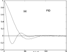
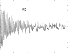
Figure 12: (a) Free induction decay of a single crystal of calcium fluoride, at two different crystal orientations (b) Decay of the ¹⁹F signal while the dipolar coupling between the nuclear spins is decoupled. (The sequence was modified to show an oscillation, so the decoupling is not optimal here.)

The decay of the observed FID in Figure 12(a) is due to the mutual dipolar couplings of the spins. These couplings produce correlated many spin states that are not directly observable using standard NMR techniques. However, using multiple quantum encoding techniques c69 , it is possible to directly measure the growth of the spin system under the dipolar coupling. The truncated dipolar Hamiltonian shown above is a zero quantum Hamiltonian when examined in the basis of the quantizing Zeeman Hamiltonian as expected. However, we can requantize the system in another basis (such as the $x$-basis for example) via a similarity transformation, and explore the growth of multiple quantum coherences in this new basis. The dipolar Hamiltonian in the $x$-basis is

$${\cal H}=-\frac{1}{2}\sum_{i<j}d_{ij}\left\{2I_{x}^{i}I_{x}^{j}-\frac{1}{2}\left(I_{x+}^{i}I_{x-}^{j}+I_{x-}^{i}I_{x+}^{j}\right)\right\}-\frac{3}{4}\sum_{i<j}d_{ij}\left(I_{x+}^{i}I_{x+}^{j}+I_{x-}^{i}I_{x-}^{j}\right)$$ (21)

and is thus seen to contain both zero and double quantum terms. It is possible to directly observe the growth of these $x$-basis coherences. Figure 13 shows the results of this experiment, illustrating the growth in the number of the correlated spins from 1 to about 20 in the first 150 $\mu$s following the application of a $\pi$/2 pulse.

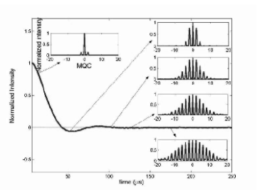
Figure 13: Multiple quantum encoding, combined with evolution reversal sequences allow us to follow the growth of the correlated spin states during the course of a free induction decay. It is seen that even when the macroscopic signal appears to have decayed away, the spin system remains highly coherent, and states involving up to 20 correlated spins are observed.

In an early demonstration of the capability to explore many body dynamics in spin systems, solid state NMR techniques have been used to directly measure the rate of spin diffusion of Zeeman and dipolar energy in a single crystal of calcium fluoride c70 ; c71 . As seen from the Hamiltonian above, these are both constants of the motion and are independently conserved. Spin diffusion is a coherent process caused by the mutual spin flips induced by the dipolar coupling between spins, that appears diffusive in the long-time, long-wavelength limit c72 . It is estimated that up to $10^{18}$ spins are involved at the long timescales explored in these experiments. It was found that while the measured diffusion coefficients for Zeeman order were in good agreement with theoretical predictions, the diffusion of dipolar order was observed to be significantly faster than previously predicted. While these experiments were performed in highly mixed thermal states, future experiments planned at low temperatures, and high polarizations should enable a more complete exploration of the large Hilbert space dynamics.

VII Conclusions

NMR implementations of QIP have thus yielded a wealth of information by providing experimental realizations of a number of proposed schemes. This in turn has guided our understanding of the relevant issues involved in scaling these testbed systems up in size. The methodologies developed are relevant across most of the physical platforms that have been proposed for QIP, and manifestations of this ”cross-fertilization” are beginning to appear in the literature.

Solid state NMR holds great promise for scalable QIP architectures. The efforts currently underway to characterize and control large spin systems are essential to determining how the methodologies of control and system decoherence scale as a function of the system Hilbert space size.

VIII Acknowledgements

This work was supported by funds from ARDA/ARO (DAAD19-01-1-0519), DARPA (MDA972-01-1-0003), the NSF (EEC 0085557) and the Air Force Office of Sponsored Research.

References

- (1) B. E. Kane, Nature 393, 133 (1998).
- (2) G. Burkard, H.-A. Engel, D. Loss, Fortschr. Phys. 48, 965 (2000).
- (3) A. Imamoglu, Fortschr. Phys. 48, 987 (2000).
- (4) V. Privman, I. D. Vagnet, G. Kventsel, Phys. Lett. A 239, 146 (1998).
- (5) D. G. Cory, R. Laflamme, E. Knill, L. Viola, T.F. Havel, N. Boulant, G. Boutis, E. Fortunato, S. Lloyd, R. Martinez, C. Negrevergne, M. Pravia, Y. Sharf, G. Teklemariam, Y. S. Weinstein and W.H. Zurek, Fortschr. Phys. 48, 875 (2000).
- (6) J. Wrachtrup, S. Y. Kilin and A. P. Nizovtsev, Opt. Spectrosc+ 91, 429 (2001).
- (7) G. P. Berman, G. W. Brown, M. E. Hawley, V. I. Tsifrinovich, Phys. Rev. Lett. 87, 097902 (2001).
- (8) T. D. Ladd, J. R. Goldman, F. Yamaguchi, Y. Yamamoto, Phys. Rev. Lett. 89, 017901 (2002).
- (9) E. Abe, K. M. Itoh, T. D. Ladd, J. R. Goldman, F. Yamaguchi and Y. Yamamoto, J. Superconductivity 16, 175 (2003).
- (10) D. Suter and K. Lim, Phys. Rev. A 65, 052309 (2002).
- (11) C.P. Slichter, Principles of Magnetic Resonance, 3rd Edition, Springer-Verlag, Berlin (1990).
- (12) R. R. Ernst, G. Bodenhausen, A. Wokaun, Principles of Nuclear Magnetic Resonance in One and Two Dimensions, Oxford University Press, Oxford (1990).
- DiVincenzo (2000) D. P. DiVincenzo, Fortschr. Physik 48, 771 (2000).
- Cory et al. (1997) D. G. Cory, A. F. Fahmy, and T. F. Havel, Proc. Natl. Acad. Sci. USA 94, 1634 (1997).
- Gershenfeld and Chuang (1997) N. Gershenfeld and I. L. Chuang, Science 275, 350 (1997).
- Warren (1997) W. Warren, Science 277, 1688 (1997).
- Schulman and Vazirani (1998) L. J. Schulman and U. Vazirani, arXive eprint quant-ph/9804060 (1998).
- Chang et al. (2001) D. Chang, L. Vandersypen, and M. Steffen, Chem. Phys. Lett. 338, 337 (2001).
- Yannoni et al. (1999) C. Yannoni, M. Sherwood, L. Vandersypen, M. Kubinec, D. Miller, and I. Chuang, Appl. Phys. Lett. 75, 3563 (1999).
- Marjanska et al. (2000) M. Marjanska, I. Chuang, and M. Kubinec, J. Chem. Phys. 112, 5095 (2000).
- Vandersypen et al. (2000a) L. Vandersypen, M. Steffen, G. Breyta, C. Yannoni, R. Cleve, and I. L. Chuang, Phys. Rev. Lett. 85, 5452 (2000a).
- Deutsch and Jozsa (1992) D. Deutsch and R. Jozsa, Proc. R. Soc. Lond. A 439, 553 (1992).
- Simon (1994) D. Simon, in Proc. 35th Annual Symposium on Foundations of Computer Science (IEEE Computer Society Press, Los Alamitos, CA, 1994), pp. 116–123.
- Kitaev (1995) A. Y. Kitaev, LANL E-print quant-ph/9511026 (1995).
- (25) H. K. Cummins, and J. Jones, New. J. Phys. 2, 6.1-6.12 (2000).
- Jones (2003) J. Jones, arXive e-print quant-ph/0301019 (2003).
- (27) M. A. Pravia, N. Boulant, J. Emerson, E. Fortunato, T. F. Havel and D. G. Cory, J. Chem. Phys. 119, 9993 (2003).
- (28) N. Boulant, S. Furuta, J. Emerson, T. F. Havel and D. G. Cory, in preparation.
- (29) U. Haeberlen and J. S. Waugh, Phys. Rev. 175, 453 (1968).
- (30) S. J. Glaser, T. Schulte-Herbruggen, M. Sieveking, O. Schedletzky, N. C. Nielsen, O. W. Sorensen and C. Griisigner, Science 280, 421 (1998).
- (31) M. Levitt, Prog. Nucl. Magn. Reson. Spectrosc. 18, 61 (1986).
- (32) A. Shaka and R. Freeman, J. Magn. Reson. 55, 487 (1983).
- (33) J. Baum, R. Tycko and A. Pines, Phys. Rev. A 32, 3435 (1985).
- (34) M. S. Silver, R. I. Joseph and D. I. Hoult, Phys. Rev. A 31, 2753 (1985).
- (35) H. Cummins, G. Llewellyn and J. Jones, Phys. Rev. A 67, 042308 (2003).
- (36) R. Tycko, A. Pines and J. Guckenherimer, J. Chem. Phys. 83, 2775 (1985).
- (37) E. M. Fortunato, M. A. Pravia, N. Boulant, G. Teklemariam, T. F. Havel and D. G. Cory, J. Chem. Phys. 116, 7599 (2002).
- Vandersypen and Chuang (2004) L. Vandersypen and I. L. Chuang, Rev. Mod. Phys. in press (2004).
- Knill et al. (2000) E. Knill, R. Laflamme, R. Martinez, and C.-H. Tseng, Nature 404, 368 (2000).
- (40) D. Stefanatos, N. Khaneja and S. J. Glaser, Phys. Rev. A 69, 022319 (2004).
- (41) N. Khaneja, S. J. Glaser and R. Brockett, Phys. Rev. A 65, 032301 (2002).
- (42) N. Khaneja, R. Brockett and S. J. Glaser, Phys. Rev. A 63, 032308 (2001).
- (43) K. Kraus, Ann. Phys. 64, 311 (1971).
- (44) E. L. Hahn, Phys. Rev. 80, 580 (1950).
- (45) H. Y. Carr and E. M. Purcell, Phys. Rev. 93, 749 (1954).
- (46) R. Tycko, H. M. Cho, E. Schneider, and A. Pines, J. Magn. Reson. A 61 90 (1980).
- (47) R. Tycko, Phys. Rev. Lett. 51, 775 (1983).
- (48) J. S. Waugh, J. Mag. Res. 50, 30 (1982).
- (49) E. Knill, R. Laflamme and L. Viola, Phys. Rev. Lett. 84, 2525 (2000).
- (50) L. Viola, E. Knill and S. Lloyd, Phys. Rev. Lett. 82, 2417 (1999).
- (51) L. Viola and S. Lloyd, Phys. Rev. A. 58, 2733 (1998).
- (52) A. M. Childs, I. L. Chuang and D. W. Leung, Phys. Rev. A 64, 012314 (2001).
- (53) N. Boulant, T. F. Havel, M. A. Pravia and D. G. Cory, Phys. Rev. A 67, 042322 (2003).
- (54) Y. Weinstein, T. F. Havel, J. Emerson, N. Boulant, M. Saraceno, S. Lloyd and D. G. Cory, to be submitted
- (55) P. Shor, Phys. Rev. A 52, 2493 (1995).
- (56) A. M. Steane, Phys. Rev. Lett. 77, 793 (1996).
- (57) J. Preskill, Proc. Roy. Soc. London A 454, 385 (1998).
- (58) M. A. Nielsen and I. L. Chuang, Quantum Computation and Quantum Information Cambridge University Press, Cambridge, 2000.
- (59) L. Viola, E. M. Fortunato, M. A. Pravia, E. Knill, R. Laflamme and D. G. Cory, Science 293, 2059 (2001).
- (60) D. G. Cory, M. D. Price, W. Maas, E. Knill, R. Laflamme, W. H. Zurek, T. F. Havel and S. S. Somaroo, Phys. Rev. Lett. 81, 2152 (1998).
- (61) E. M. Fortunato, L. Viola, J. Hodges, G. Teklemariam and D. G. Cory, New J. Phys. 4, 5.1-5.20 (2002).
- (62) N. Boulant, M. A. Pravia, E. M. Fortunato, T. F. Havel and D. G. Cory, QIP 1, 135 (2002).
- (63) E. Knill, R. Laflamme, R. Martinez and C. Negrevergne, Phys. Rev. Lett. 86, 5811 (2001).
- (64) D. Leung, L. Vandersypen, X. Zhou, M. Sherwood, C. Yannoni, M. Kubinec and I. L. Chuang, Phys. Rev. A 60, 1924 (1999).
- (65) J. E. Ollerenshaw, D. A. Lidar and L. E. Kay, Phys. Rev. Lett. 91, 217904 (2003).
- Chuang et al. (1998a) I. L. Chuang, N. Gershenfeld, and M. Kubinec, Phys. Rev. Lett. 18, 3408 (1998a).
- Jones et al. (1998) J. A. Jones, M. Mosca, and R. H. Hansen, Nature 393, 344 (1998), quant-ph/9805069.
- Chuang et al. (1998b) I. L. Chuang, L. M. K. Vandersypen, X. L. Zhou, D. W. Leung, and S. Lloyd, Nature 393, 143 (1998b).
- Jones and Mosca (1998) J. A. Jones and M. Mosca, J. Chem. Phys. 109, 1648 (1998), arXive e-print quant-ph/9801027.
- Jones and Mosca (1999) J. Jones and M. Mosca, Phys. Rev. Lett. 83, 1050 (1999).
- Vandersypen et al. (1999) L. M. K. Vandersypen, C. S. Yannoni, M. H. Sherwood, and I. L. Chuang, Phys. Rev. Lett. 83, 3085 (1999).
- Vandersypen et al. (2000b) L. Vandersypen, M. Steffen, M. H. Sherwood, C. Yannoni, G. Breyta, and I. L. Chuang, Appl. Phys. Lett. 76, 646 (2000b).
- Linden et al. (1998) N. Linden, H. Barjat, and R. Freeman, Chem. Phys. Lett 296, 61 (1998).
- Collins et al. (2000) D. Collins, N. Linden, and S. Popescu, arXive eprint quant-ph/0005102 (2000).
- Kim et al. (2000) H. Kim, J.-S. Lee, and S. Lee, Phys. Rev. A 62, 022312 (2000).
- Marx et al. (2000) R. Marx, A. Fahmy, J. Myers, W. Bermel, and S. Glaser, Phys. Rev. A 62, 123310 (2000).
- Weinstein et al. (2001) Y. Weinstein, M. Pravia, E. Fortunato, S. Lloyd, and D. Cory, Phys. Rev. Lett. 86, 1889 (2001).
- Vandersypen et al. (2001) L. Vandersypen, M. Steffen, G. Breyta, C. Yannoni, R. Cleve, and I. L. Chuang, Nature 414, 883 (2001).
- Steffen et al. (2003a) M. Steffen, W. van Dam, T. Hogg, G. Breyta, and I. Chuang, Phys. Rev. Lett. (2003a).
- Farhi and Goldstone (2001) E. Farhi and J. Goldstone, Science 292, 472 (2001).
- Hogg (2000) T. Hogg, Phys. Rev. A 61, 052311 (2000).
- Laflamme et al. (1998) R. Laflamme, E. Knill, W. H. Zurek, P. Catasti, and S. V. S. Mariappan, Phil. Trans. Roy. Soc. Lond. A 356, 1941 (1998), arXive e-print quant-ph/9709025.
- Braunstein et al. (1999) S. L. Braunstein, C. M. Caves, R. Jozsa, N. Linden, S. Popescu, and R. Schack, Phys. Rev. Lett. 83, 1054 (1999).
- Nelson et al. (2000) R. Nelson, D. Cory, and S. Lloyd, Phys. Rev. A 61, 022106(5) (2000).
- Nielsen et al. (1998) M. A. Nielsen, E. Knill, and R. Laflamme, Nature 396, 52 (1998).
- Fang et al. (2000) X. Fang, X. Zhu, M. Feng, X. Mao, and F. Du, Phys. Rev. A 61, 022307(5) (2000).
- Cummins et al. (2002) H. K. Cummins, G. Llewellyn, and J. Jones, arXive eprint quant-ph/0208092 (2002).
- Weinstein et al. (2002) Y. Weinstein, S. Lloyd, J. Emerson, and D. Cory, Phys. Rev. Lett. 89, 157902 (2002).
- Verhulst et al. (2001) A. Verhulst, O. Liivak, H. Vieth, C. Yannoni, and I. Chuang, Appl. Phys. Lett. 79, 2480 (2001).
- Hübler et al. (2000) P. Hübler, J. Bargon, and S. Glaser, J. Chem. Phys. 113, 2056 (2000).
- (91) J. A. Jones, arXiv E-print quant-ph/0312014.
- (92) R. Feynman, Int. J. Theor. Phys. 21, 467 (1982).
- (93) S. Somaroo, C. H. Tseng, T. F. Havel, R. Laflamme and D. G. Cory, Phys. Rev. Lett. 82, 5381 (1999).
- (94) D. Bacon, A. M. Childs, I. L. Chuang, J. Kempe, D.W. Leung, and X.L. Zhou, Phys. Rev. A 64, 062302 (2001).
- (95) W. H. Zurek, Phys. Rev. D 26, 1862 (1982)
- (96) G. Teklemariam, E. M. Fortunato, C. C. Lopez, J. Emerson, J. P. Paz, T. F. Havel and D. G. Cory, Phys. Rev. A 67, 062316 (2003)
- (97) J. Yepez, Int. J. Mod. Phys. C9, 1587 (1998)
- (98) J. Yepez, Int. J. Mod. Phys. C12, 1285 (2001)
- (99) M. A. Pravia, Z. Chen, J. Yepez and D. G. Cory, QIP 2, 97 (2003)
- Wimperis (1994) S. Wimperis, J. Magn. Reson. B 109, 221 (1994).
- Gulde et al. (2003) S. Gulde, M. Riebe, G. Lancaster, C. Becher, J. Eschner, H. Häffner, F. Schmidt-Kaler, I. Chuang, and R. Blatt, Nature 421, 48 (2003).
- (102) E. Collin, G. Ithier, A. Aasime, P. Joyez, D. Vion, D. Esteve, LANL E-print cond-mat/0404507.
- Pauly et al. (1991) J. Pauly, P. L. Roux, and D. Nishimura, IEEE Trans. Med. Imag. 10, 53 (1991).
- Warren (1984) W. Warren, J. Chem. Phys. 81, 5437 (1984).
- Green and Freeman (1991) M. Green and R. Freeman, J. Magn. Reson. 93, 93 (1991).
- Steffen et al. (2003b) M. Steffen, J. Martinis, and I. L. Chuang, Phys. Rev. B 68, 224518 (2003b).
- (107) P. O. Boykin, T. Mor, V. Roychowdhury, F. Vatan and R. Vrijen, Proc. Natl. Acad. Sci. 99, 3388 (2002).
- (108) S. Lloyd, Science 261, 1569 (1993).
- (109) M. Mehring, J. Mende andW. Scherer, Phys. Rev. Lett. 90, 153001 (2003).
- (110) G. M. Leskowitz, N. Ghaderi, R. A. Olsen and L. J. Mueller, J. Chem. Phys. 119, 1643 (2003).
- (111) G. S. Boutis, P. Cappellaro, H. Cho, C. Ramanathan and D. G. Cory, J. Magn. Reson. 161, 132 (2003).
- (112) C. Ramanathan, H. Cho, P. Cappellaro, G. S. Boutis, D. G. Cory, Chem. Phys. Lett. 369, 311 (2003).
- (113) W. Zhang, D. G. Cory, Phys. Rev. Lett. 80, 1324 (1998).
- (114) G. S. Boutis, D. Greenbaum, H. Cho, D. G. Cory and C. Ramanathan, Phys. Rev. Lett. 92, 137201 (2004).
- (115) N. Bloembergen, Physica (Amsterdam) 15, 386 (1949).