We study the decay process of an unstable quantum system, especially the deviation from the exponential decay law. We show that the exponential period no longer exists in the case of the s-wave decay with small $Q$ value, where the $Q$ value is the difference between the energy of the initially prepared state and the minimum energy of the continuous eigenstates in the system. We also derive the quantitative condition that this kind of decay process takes place and discuss what kind of system is suitable to observe the decay.

I    INTRODUCTION

Since the period of the classic works by Dirac [1] and Weisskopf and Wigner [2], it has been a problem how to describe the decay process of an unstable state following the principles of quantum mechanics. As is well known, the survival probability of the initial state $P(t)$, which concerns the decay of the quantum state, is frequently described by the exponential decay law $P(t)=e^{-\Gamma t}$. However, it is also known that the decay process does not obey the exponential law precisely, so it has always been a question of how the deviation from the exponential decay law occurs, especially at the late and early times of a decay process [3].

Theorists are always motivated to work on this old problem when high-resolution experiments, which are accomplished by a new technology, are performed to detect the deviation of the decay law from the exponential [4] - [6]. In addition, recent several experiments have reported the measurement-induced suppression in quantum systems at the early stage of decay, which may be a result of the Quantum Zeno Effect (QZE) [7].

As mentioned above, the deviation from the exponential law at late and early times is often discussed [8, 9]. At very late times, the survival probability $P(t)$ must decrease more slowly than the exponential and exhibits the inverse power law of time $P(t)\sim t^{-\alpha}$, where $\alpha$ is positive and depends on the property of the unstable system. At early times, the survival probability decreases following a Gaussian law (the square of time $t^{2}$), which appears inevitably in a quantum process (and causes the QZE). Thus the decay of the unstable state proceeds through three stages in general. The initial stage is characterized by a Gaussian law, the intermediate stage by an exponential law, and the final stage by an inverse power law.

In this paper we focus on a different mechanism of deviation from the exponential law. Such a decay process occurs in the case of small-$Q$-value s-wave decay (SQS decay). Here the $Q$ value is defined by the difference between the energy of the initially prepared state (denoted by $E_{0}$) and the minimum energy of the continuous eigenstates (denoted by $E_{th}$) in the system. The small-$Q$-value decay has been discussed in some papers [9, 10]. The point we would like to emphasize here is as follows: in the case of the SQS decay, we can observe not only the enhancement of the QZE, but also no exponential period. This means that the deviation from the exponential law can be observed easily if the SQS decay system is prepared. We also derive the quantitative condition that such a decay takes place.

This paper is organized as follows. In Sec.II, we show an example of the SQS decay by using the one-dimensional tunneling system with a box-type potential. The general description for an unstable system is formulated in Sec.III. Using this formalism, we derive the quantitative condition that the SQS decay occurs in Sec.IV. In Sec.V, we summarize our results and discuss what kind of system exhibits such a decay process.

II    AN EXAMPLE OF SQS DECAY IN TUNNELING PHENOMENA

Before going into the general discussion, we show the example of SQS decay in the tunneling phenomena. In this section we discuss the one-dimensional tunneling problem because only the radial part of the wave function is relevant to the s-wave tunneling even in a three-dimensional system.

Let us consider the decay process through the one-dimensional box-type potential depicted in Fig.1. Parameters for characterizing the system are also shown in the figure. Here we assume $U_{0}$ is not so large that there is no bound state. The goal here is to calculate the survival probability of the prepared state and show that the SQS decay is realized in this system.

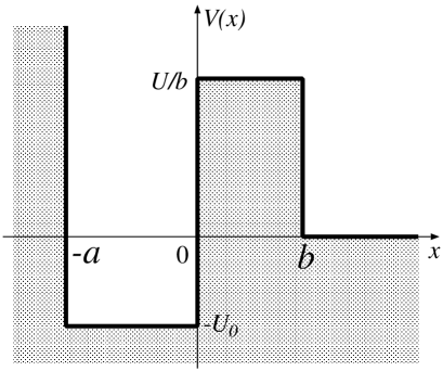
Figure 1: The shape of the potential.

The survival probability $P(t)$ is defined by the nondecay amplitude $a(t)$ as $P(t)=|a(t)|^{2}$. $a(t)$ is given by

$$a(t)\equiv\langle 0|e^{iHt}|0\rangle~{},$$ (1)

where $|0\rangle$ is the initially prepared state and $H$ is the Hamiltonian of the system. Please note that we use the units $\hbar=1$ in this paper. The nondecay amplitude can be expanded over the energy eigenstates $|E\rangle$ as

$$a(t)=\int_{0}^{\infty}dE~{}\rho(E)~{}e^{-iEt}~{},\qquad\rho(E)=|\langle E|0\rangle|^{2}~{}.$$ (2)

The function $\rho(E)$ is called the spectral function, in which all information about the decay process is included. The energy eigenstate $|E\rangle$ can be obtained analytically in this system as detailed in Appendix A. Here we take the initial state $|0\rangle$ as the ground state in the well for the infinitely height barrier,

$$\psi_{i}(x)\equiv\langle x|0\rangle=\sqrt{\frac{2}{a}}\sin{\left(\frac{\pi x}{a}\right)}\theta(x+a)\theta(-x)~{}.$$ (3)

The energy expectation value of this state is $E_{0}\equiv\pi^{2}/(2ma^{2})-U_{0}$ and the $Q$ value is given by $Q\equiv E_{0}-E_{th}=\pi^{2}/(2ma^{2})-U_{0}$ because the spectrum of the continuum energy eigenstate starts from the zero energy. Using this initial wave function, the spectral function of the system is obtained analytically after some calculations, and given by

$$\rho(E)=\frac{1}{2ma^{2}\alpha(E)}\frac{2\pi q\sin^{2}r}{(r^{2}-\pi^{2})^{2}}~{},$$ (4)

where

$$\alpha(E)=q^{2}+G_{0}\cos^{2}r-\frac{G}{u}\sin^{2}r+\frac{G}{u}\left(\frac{r}{s}\cos r\cdot\sinh(su)+\sin r\cdot\cosh(su)\right)^{2}\!\!\!,$$ (5)

for the case that the energy is smaller than the potential barrier $E\leq U/b$, while

$$\alpha(E)=q^{2}+G_{0}\cos^{2}r-\frac{G}{u}\sin^{2}r+\frac{G}{u}\left(\frac{r}{\tilde{s}}\cos r\cdot\sin(\tilde{s}u)+\sin r\cdot\cos(\tilde{s}u)\right)^{2}.$$ (6)

for the other case $E\geq U/b$. Here we use the dimensionless quantities to write down the spectral function $q=\sqrt{2mE}a$, $r=\sqrt{2m(E+U_{0})}a$, $s=\sqrt{2m(U/b-E)}a$, and $\tilde{s}=\sqrt{2m(E-U/b)}a$. Furthermore, the variables that characterize the potential are also given by the dimensionless ones $G=2maU$, $G_{0}=2ma^{2}U_{0}$, and $u=b/a$.

For investigating the SQS decay, we define the decay rate $\Gamma(t)$ by

$$\Gamma(t)=-\frac{d}{dt}\ln P(t)~{}.$$ (7)

This quantity is more convenient rather than the survival probability itself because this rate is constant while the decay process is governed by the exponential law. We performed the integral in Eq.(2) numerically using the spectral function Eq.(4), and calculated the decay rate $\Gamma(t)$. The results are shown in Fig.2. We studied two cases of $G_{0}$, that is, $G_{0}=0$ and $8.957335$ which correspond to the cases $Q=8.97365$ and $6.55445\times 10^{-4}$ [the units of $Q$ are $(2ma^{2})^{-1}$], with fixed $G$ and $U$. As you see, the exponential decay law is observed in the case that the $Q$ value is not very small. On the other hand, if the $Q$ value is small enough the exponential period no longer exists even at the time $t\sim 500(2ma^{2})$ when $P(t)$ decreases to the order of $e^{-1}$. This is nothing but an example of the SQS decay.

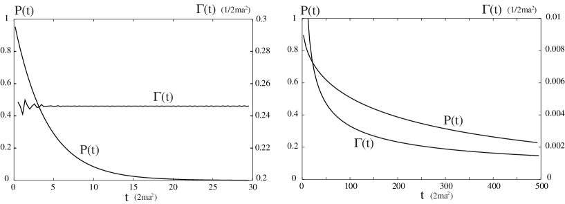
Figure 2: Examples of decay. Here we set $G=20,G_{0}=0$ (or $Q=8.97365(2ma^{2})^{-1}$), $u=10^{-4}$ on the left and $G=20,G_{0}=8.957335$ (or $Q=6.55445\times 10^{-4}(2ma^{2})^{-1}$), $u=10^{-4}$ on the right. Each quantity in the figure is averaged over a short time interval. The example on the right corresponds to the SQS decay.

In the following sections we investigate the SQS decay by a general description and what kind of situation is necessary. We also derive the quantitative condition for the SQS decay to take place.

III    GENERAL DESCRIPTION FOR UNSTABLE STATE

In this section we explain the general formalism of unstable state decay. Using this formalism the quantitative condition for the SQS decay is derived in the next section.

For calculating the nondecay amplitude we use an exact integro-differential equation by using the technique in Refs. [11, 9]. We introduce the projector onto the initial unstable state, ${\cal P}\equiv|0\rangle\langle 0|$, and decompose the Hamiltonian $H$ as

$$H = H_{0}+V~{},$$

$$H_{0} \equiv {\cal P}H{\cal P}+(1-{\cal P})H(1-{\cal P})~{},\qquad V\equiv H-H_{0}~{}.$$ (8)

Define the energy eigenstates $|a\rangle$ of $H_{0}$; $H_{0}|a\rangle=E_{a}|a\rangle$. It is then easy to confirm that the decay interaction $V$ operates only between the initial state $|0\rangle$ and its orthogonal complement $|n\rangle$; $V_{0n}=V_{n0}^{*}\neq 0$, $V_{mn}=V_{00}=0$. Here we use the intermediate roman letters such as $m$, $n$ to denote eigenstates projected by $1-{\cal P}$. The interaction $V$ depends on the initially prepared state. Although this formalism looks odd, we can execute an exact analysis like a time development of the unstable state using this tool.

We work in the interaction picture and expand the state at a finite time $t$, using the basis of the eigenstate of $H_{0}$; $|\psi\rangle_{I}=e^{iH_{0}t}|\psi\rangle=\sum_{a}c_{a}(t)|a\rangle$. We thus write the time evolution equation for the coefficient $c_{a}(t)$:

$$i\dot{c}_{0}=\sum_{n}~{}V_{0n}~{}e^{-i(E_{n}-E_{0})t}~{}c_{n}~{},\qquad i\dot{c}_{m}=V_{m0}~{}e^{i(E_{m}-E_{0})t}~{}c_{0}~{}.$$ (9)

Here $E_{0}$ is the energy of the initial unstable state; $E_{0}=\langle 0|H|0\rangle$. The nondecay amplitude is related to this coefficient by $\langle 0|e^{-iHt}|0\rangle=e^{-iE_{0}t}c_{0}(t)$. From the above equations, a closed form of the equation for the nondecay amplitude $c_{0}(t)\equiv a(t)$ then follows:

$$\dot{a}(t) = -\int_{0}^{t}~{}dt~{}\beta(t-t^{\prime})~{}a(t^{\prime})~{},$$ (10)

$$\beta(t-t^{\prime}) = \langle 0|V_{I}(t)V_{I}(t^{\prime})|0\rangle=\int_{E_{th}}^{\infty}~{}dE~{}\sigma(E)~{}e^{-i(E-E_{0})(t-t^{\prime})}~{},$$ (11)

$$\sigma(E) = \sum_{m}\delta(E-E_{m})|V_{0m}|^{2}~{}.$$ (12)

Here $V_{I}(t)=e^{iH_{0}t}~{}V~{}e^{-iH_{0}t}$ is the decay interaction written in the interaction picture and the function $\sigma(E)$ characterizes the interaction between the unstable state $|0\rangle$ and the other states $|m\rangle$. The initial condition $c_{m}(0)=0$ is used to derive the equation for $a(t)$, and $E_{th}$ is the threshold for the state $|m\rangle$.

The standard technique to solve this type of integro-differential equation (10) is the one that utilizes the Laplace transform, and we finally obtain the nondecay amplitude in the form

$$a(t) = \int_{-\infty}^{\infty}\frac{dE}{2\pi i}F(E+i0^{+})~{}e^{-i(E-E_{0})t}~{},$$ (13)

$$F(z) \equiv \frac{1}{-z+E_{0}-G(z)}~{},\qquad G(z)=\int_{E_{th}}^{\infty}dE\frac{\sigma(E)}{E-z}~{}.$$ (14)

The initial condition $a(0)=1$ is imposed in this derivation.

The analytic property of the function $F(z)$ is evident; this function is analytic except on the branch cut which runs from the threshold value $E_{th}$ to positive infinity on the real axis (Fig.3). As is well known, if the Riemann surface is considered by analytic continuation through the branch cut (and regarding the original complex $z$ plane as the first Riemann sheet), there is a pole on the second Riemann sheet near and below the real axis if the decay interaction is weak enough. The pole location $z_{p}$ is determined by

$$z_{p}-E_{0}+G_{II}(z_{p})=z_{p}-E_{0}+\int_{E_{th}}^{\infty}dE\frac{\sigma(E)}{E-z_{p}}+2\pi i\sigma(z_{p})=0~{},$$ (15)

where the analytic function $G(z)$, and hence $F(z)$, is extended into the second sheet by $G_{II}(E-i0^{+})=G_{I}(E+i0^{+})$ through the branch cut. The real function $\sigma(E)$, which was originally defined for real $E>E_{th}$, is also extended to the function $\sigma(z)$ defined on the complex plane by analytic continuation. In addition to this pole there may be some singularities on the second Riemann sheet, but we ignore the effects of such singularities in the following discussion. This approximation is valid as discussed in Ref. [9] because these singularities do not affect the decay phenomena except for the early stage.

Using the discontinuity of the analytic function $F(z)$ across the branch cut on the first Riemann sheet,

$$F(E+i0^{+})-F(E-i0^{+})=2\pi i\sigma(E)~{}|F(E+i0^{+})|^{2}~{},$$ (16)

which is called the ”elastic” unitarity relation, we can deform the contour of integration on the real axis in Eq.(13) into the sum of two contours, one around the pole as shown by $C_{p}$ and the other along $C_{th}$ in Fig.3,

$$a(t)=\left(\int_{C_{p}}+\int_{C_{th}}\right)\frac{dz}{2\pi i}F(z)~{}e^{-i(z-E_{0})t}~{}.$$ (17)

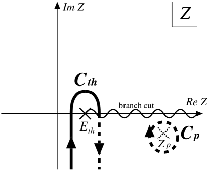
Figure 3: The analytic structure of the complex $z$ plane and the contours of the integrals. The contours and the pole shown by the broken line are on the second Riemann sheet.

We consider the case that the unstable state initially prepared is a metastable state, which means the decay interaction is weak in comparison with the typical energy of the system, $E_{sys}$, induced from the oscillation in the well: $\sigma\ll E_{sys}\sim E_{0}$. Then the pole location on the second Riemann sheet can be obtained approximately as

$$z_{p}\simeq E_{0}-\Pi(E_{0})-i\pi\sigma(E_{0})~{},\qquad\Pi(E)={\rm p.v.}\int_{E_{th}}^{\infty}dE^{\prime}\frac{\sigma(E^{\prime})}{E^{\prime}-E}~{},$$ (18)

where p.v. means the principal value of the integration. The $C_{p}$ integration in Eq.(17) can be performed without difficulty by the residue theorem, and with the aid of the approximation above, this becomes

$$\int_{C_{p}}\frac{dz}{2\pi i}F(z)~{}e^{-i(z-E_{0})t}\simeq e^{i\Pi(E_{0})t}e^{-\pi\sigma(E_{0})t}~{}.$$ (19)

This integration gives an ${\cal O}(1)$ contribution to the nondecay amplitude $a(t)$. On the other hand, the integration along $C_{th}$ is of ${\cal O}(\sigma/E_{0})$, which gives only a small contribution. This is because the integration can be approximated by

$$\int_{C_{th}}\frac{dz}{2\pi i}F(z)~{}e^{-i(z-E_{0})t} = -ie^{i(E_{0}-E_{th})t}\int^{\infty}_{0}dy~{}\sigma(E_{th}-iy)|F(E_{th}-iy)|^{2}~{}e^{-yt}~{},$$ (20)

$$\simeq -ie^{i(E_{0}-E_{th})t}|F(E_{th})|^{2}\int^{\infty}_{0}dy~{}\sigma(E_{th}-iy)~{}e^{-yt}~{},$$

for sufficiently large $t$, and the factor $|F(E_{th})|^{2}$ usually takes the value $(E_{0}-E_{th})^{-2}$.

The dominance of the $C_{p}$ integration in Eq.(17) leads to the exponential decay law

$$P(t)=|a(t)|^{2}\simeq\exp(-\Gamma_{p}t)~{},\qquad\Gamma_{p}=2\pi\sigma(E_{0})~{},$$ (21)

and this coincides with the familiar golden rule of perturbation theory. From this investigation, we know that the perturbative calculation gives satisfactory results in many cases. We would, however, like to elucidate the time evolution in finer detail, and study the conditions for breaking the exponential decay law, especially the SQS decay, in the next section.

IV    THE CONDITION FOR THE SQS DECAY LAW

We now derive the quantitative condition of SQS decay. We also discuss the situations in general that exhibit deviations from the exponential decay law.

The $C_{p}$ integration around the pole $z_{p}$ in Eq.(17) always yields exponential time dependence, so nonexponential decay is realized when the $C_{th}$ integration contributes to the nondecay amplitude $a(t)$ by the same order as the $C_{p}$ integration.

From the evaluation of the contour integrations in Eq.(17), we can classify the nonexponential decays that satisfy the condition mentioned above into three cases. In the following we describe them in detail.

The first one concerns the short time behavior and is known as the QZE. At early times ($t\leq E_{sys}^{-1}$), the approximation used in Eq.(20) is no longer valid and the high-frequency component of $\sigma(E)$ becomes important. From the definition of the survival probability, we naively expect that the short time behavior exhibits a deviation from the exponential law, which is in the form of

$$|\langle 0|e^{-iHt}|0\rangle|^{2}\simeq 1-t^{2}\,\left(\langle 0|H^{2}|0\rangle-\langle 0|H|0\rangle^{2}\right)~{}.$$ (22)

Thus quantum mechanics appears to predict a quadratic form of deviation in the $t\rightarrow 0$ limit.

The second one relates to the long time behavior. At late times $t\gg 1/\Gamma_{p}$ the $C_{p}$ integration is exponentially suppressed, while the $C_{th}$ integration is not strongly suppressed because the behavior of $\sigma(E)$ near the threshold is expressed by $\sigma(E)=c(E-E_{th})^{\alpha}$, which leads to power law behavior of the $C_{th}$ integration,

$$\int_{C_{th}}\frac{dz}{2\pi i}F(z)~{}e^{-i(z-E_{0})t} \simeq -ie^{i(E_{0}-E_{th})t}|F(E_{th})|^{2}\frac{c~{}\Gamma(\alpha+1)~{}e^{-i\pi\alpha/2}}{t^{\alpha+1}}~{}.$$ (23)

Here $\Gamma(z)$ is Euler’s gamma function. Therefore the contribution from the $C_{th}$ integration exceeds the one from the $C_{p}$ integration at late times, and the decay law changes from exponential to an inverse power law.

The small $Q~{}(=E_{0}-E_{th})$ value case is the last one on which we shall mainly focus in this paper, that is, the SQS decay. This case can be understood by investigation of the prefactor $|F(E_{th})|^{2}$ in Eq.(20) in detail:

$$|F(E_{th})|^{2}=\left[Q-\Pi(E_{th})\right]^{-2}~{}.$$ (24)

Since the function $\Pi(E_{th})$ is of ${\cal O}(\sigma)$, this factor gives $Q^{-2}$ when the $Q$ value is not very small. However, if the $Q$ value is of the same order as $\sigma$, the factor $|F(E_{th})|^{2}$ becomes large and the contribution from the $C_{th}$ integration becomes comparable with the one from the $C_{p}$ integration. In this case decay that does not include the exponential period at all can be realized, and this situation never occurs in other cases described above.

We now derive the quantitative condition that the SQS decay takes place. By virtue of the analytic property of $F(z)$, we can express the amplitude $a(t)$ in the convenient form

$$a(t)=\int_{E_{th}}^{\infty}dE\rho(E)e^{-i(E-E_{0})t}~{},\qquad\rho(E)=\frac{\sigma(E)}{(E-E_{0}+\Pi(E))^{2}+(\pi\sigma(E))^{2}}~{}.$$ (25)

The function $\rho(E)$ is the spectral function as mentioned in Sec.II. The schematic shape of $\rho(E)$ is shown in Fig.4. This function takes a real positive value when $E$ is larger than the threshold $E_{th}$. $\rho(E)$ drops quickly in the limit $E\rightarrow\infty$ because this function must satisfy the normalization condition $\int^{\infty}_{E_{th}}dE\rho(E)=1$, which is equivalent to the initial condition $a(0)=1$. In addition, $\rho(E)$ has a peak around $E\sim E_{0}$. (More precisely, the exact location and the width of the peak are determined by the real and the imaginary parts of $z_{p}$ in Eq.(15).) Therefore the dominance of the $C_{p}$ integration is equivalent to the Breit-Wigner form of $\rho(E)$ or the limit $E_{th}\rightarrow-\infty$, as you can find from the shape of $\rho(E)$.

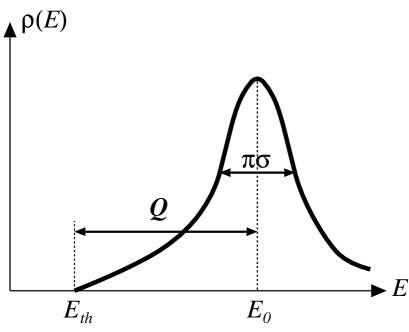
Figure 4: The typical shape of the spectral function $\rho(E)$. The SQS decay is realized when the $Q$ value is smaller than the width of the peak.

The absence of the exponential decay law due to the small $Q$ value then occurs when $Q$ is smaller than the width of the peak because the Breit-Wigner shape of $\rho(E)$ does not hold in this situation. Thus the condition for the SQS decay is given by

$$\frac{|\Im z_{p}|}{Q}\geq 1~{},\qquad Q=\Re z_{p}-E_{th}~{}.$$ (26)

This is the final result of this section, the quantitative condition for the SQS decay to take place. In Ref. [9], the authors derived the opposite condition to Eq.(26) from the viewpoint that nearly exponential decay takes place. The condition here is a necessary and sufficient condition, so our condition is consistent with theirs.

To investigate the condition Eq.(26) for a given system, this inequality is not very useful because the calculation for the exact location of $z_{p}$ from Eq.(15) is a tedious one. This situation is somewhat improved if we use the approximation Eq.(18); then the condition turns to

$$\frac{\Gamma_{p}}{E_{0}-E_{th}}\geq 2~{}.$$ (27)

This is more convenient for practical use.

As an example, we show the contour plot of $\Im z_{p}/Q$ for the model discussed in Sec.II, which is depicted in Fig.5. The contour plot is drawn on the $(G,Q)$ plane with fixed $u$. The crosses in the figure correspond to the values used in Fig.2, and in the shaded region the parameters satisfy the condition that the SQS decay takes place.

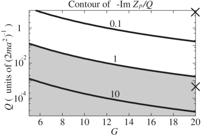
Figure 5: The value of Eq.(26) is depicted as a contour map in the $(G,Q)$ plane.

V    DISCUSSION AND SUMMARY

We now come to the stage of discussing what kind of system is necessary for the SQS decay. The important point we must pay attention to for discussing the condition Eq.(26) is the $Q$ dependence of $\Im z_{p}$, the imaginary part of the pole location. The $Q$ dependence is determined by the function $\sigma(E_{0})$ as shown in Eq.(18). When the $Q$ value is small enough, the dependence is determined by the threshold behavior of $\sigma(E_{0})$, which originates from the spectral function $\rho(E_{0})$ as shown in Eq.(25). Therefore the threshold behavior of the spectral function, taken to be $\rho(E_{0})=c(E_{0}-E_{th})^{\alpha}=cQ^{\alpha}$, is the key quantity in this problem. Here the coefficient $c$ is a constant dependent on the system. The SQS decay is expected when the power of $\rho(E_{0})$ near the threshold, $\alpha$, is smaller than 1.

As is well known, the threshold behavior of the spectral function is determined by the quantum number of the orbital angular momentum in a scattering process (e.g., a particle decay or a radioactive process), which we denote $l$ [12]. The threshold behavior is given by $\rho(E_{0})=c(E_{0}-E_{th})^{l+1/2}$. Therefore s-wave ($l=0$) decay is necessary for the SQS decay in these processes, and the SQS decay never occurs via higher-$l$ ($l\geq 1$) processes.

Let us move on to the decay process through tunneling. For the one-dimensional model discussed in Sec.II, the threshold behavior is given by

$$\rho(E_{0})=\frac{Q^{1/2}}{4\pi ma^{2}\alpha(0)}~{},\qquad Q=E_{0}-E_{th}~{},$$ (28)

which is the same as in the case of the s-wave decay. This is the very reason that the system exhibits the SQS decay when the $Q$ value is small enough. You might think that such a threshold behavior is due to a peculiarity of the potential. This is, however, not correct. To check this, let us consider a system with the modified potential shown in Fig.6. The spectral function of this system can also be obtained analytically using Bessel functions. The threshold behavior again coincides with the case of the s-wave decay. The form of the spectral function and the threshold behavior are given in Appendix B.

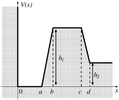
Figure 6: The modified potential.

This result is naturally understood if we consider the model with spherical symmetry in three dimensions. Since the angular momentum is a conserved quantity in this case, the s-wave decay process can always be reduced to a problem in a one-dimensional system. Therefore the threshold behaviors of all models in one dimension with nonsingular potential are the same as the one of s-wave decay.

We summarize the results of this paper. The decay of the unstable state with small $Q$ value in the s-wave process (SQS decay) exhibits the interesting feature that there is no exponential period. If we can make practical use of this mechanism, we will easily observe the deviation from the exponential law. As mentioned above, the SQS decay takes place in a system described by an s-wave process or a one-dimensional system. However it is difficult to prepare a setup of small $Q$ value in experiments on particle decay or radioactive processes, because the $Q$ values in such cases are fixed by nature and we cannot control them. On the other hand, the tunneling phenomenon may be hopeful to observe the SQS process because we may achieve sufficiently small $Q$ more easily. Unfortunately, experiments to look for the SQS decay have not been carried out until now. It is important to discuss an actual physical system which realizes the SQS decay, but this issue is beyond the scope of this paper and remains as a future problem. We believe that this kind of experiment is interesting to observe the nonexponential decay of an unstable quantum system.

Acknowledgments

The authors would like to kindly thank Professor S. Takagi for discussion. J.S. was supported by the Grants-in-Aid for Scientific Research on Priority Areas No. 16038202 and No. 14740168. K.T. was supported by the 21st Century COE Program at Tokyo Institute of Technology “Nanometer-Scale Quantum Physics”.

APPENDIX A

In this appendix, we calculate the spectral function $\rho(E)=|\langle E|0\rangle|^{2}$ of the one-dimensional model with a box-type potential that is used in Sec.II. The explicit form of the energy eigenstate $|E\rangle$ is necessary in this computation and it can be obtained analytically,

$$\phi_{E}(x)=\langle x|E\rangle=\left\{\begin{array}[]{ll}A\sin r(x/a+1)&$for$\quad(-a\leq x\leq 0)~{},\\ B\sinh(sx/a)+C\cosh(sx/a)&$for$\quad(0<x<b),\\ D\sin(qx/a)+E\cos(qx/a)&$for$\quad(b\leq x),\end{array}\right.$$ (32)

for $E<U/b$ and

$$\phi_{E}(x)=\langle x|E\rangle=\left\{\begin{array}[]{ll}A\sin r(x/a+1)&$for$\quad(-a\leq x\leq 0)~{},\\ B\sin(\tilde{s}x/a)+C\cos(\tilde{s}x/a)&$for$\quad(0<x<b),\\ D\sin(qx/a)+E\cos(qx/a)&$for$\quad(b\leq x),\end{array}\right.$$ (36)

for $E\geq U/b$. All parameters such as $a$, $b$, $q$, $r$, $s$, and $\tilde{s}$ are defined in Sec.II. The coefficients $A$, $B$, $C$, $D$, and $E$ can be determined by the junction condition at $x=-a$, $0$, $b$ and the normalization condition of the eigenstates, $\langle E|E^{\prime}\rangle=\delta(E-E^{\prime})$. For example, the coefficient $A$ is given by

$$|A|^{2}=\frac{q}{2ma^{3}\pi\alpha(E)}~{},$$ (37)

and others can be obtained similarly. The function $\alpha(E)$ is defined in Eqs.(5) and (6). The spectral function is defined by the overlap of the energy eigenstate $|E\rangle$ and the initially prepared state $|0\rangle$ given in Eq.(3). Using the eigenstate obtained above, the spectral function is computed as

$$\rho(E)=|\langle E|0\rangle|^{2}=\left|\int dx\phi_{E}(x)^{*}\psi_{i}(x)\right|^{2}=\frac{1}{2ma^{2}\alpha(E)}\frac{2\pi q\sin^{2}r}{(r^{2}-\pi^{2})^{2}}~{}.$$ (38)

APPENDIX B

In this appendix, we write down the explicit form of the spectral function of the model whose potential is depicted in Fig.6 and which is used in the discussion of Sec.V. The spectral function of this system can also be obtained analytically using Bessel functions, and the computation of the spectral function can be performed in the same way as in Appendix A. After some calculations we obtain

$$\rho(E)=\frac{1}{2ma^{3}k_{3}(|\epsilon_{1}|^{2}+|\epsilon_{2}|^{2})}\frac{\pi\sin^{2}(k_{1}a)}{(k_{1}^{2}a^{2}-\pi^{2})^{2}}~{},$$ (39)

where $k_{1}=\sqrt{2mE}$, $k_{2}=\sqrt{2m(h_{1}-E)}$, and $k_{3}=\sqrt{2m(E-h_{2})}$. All parameters characterizing the potential such as $a,\ldots,d$ and $h_{1},h_{2}$ are defined in Fig.6. The variables $\epsilon_{1}$ and $\epsilon_{2}$ are given by

$$\left(\begin{array}[]{c}\epsilon_{1}\\ \epsilon_{2}\end{array}\right)=F^{-1}(k_{3})\cdot T_{R}(z_{d})\cdot T^{-1}_{R}(z_{c})\cdot Ph\cdot F^{-1}(-ik_{2})\cdot T_{L}(z_{b})\cdot T^{-1}_{L}(z_{a})\left(\begin{array}[]{c}\delta_{1}\\ \delta_{2}\end{array}\right)~{}.$$ (44)

$L$ and $R$ appearing as the subscripts of the matrix $T$ represent the slopes of the barrier at the left and the right sides, $L=2ma^{3}h_{1}/(b-a)$, $R=2ma^{3}(h_{1}-h_{2})/(d-c)$. The matrices $F(k)$ and $T_{t}(z)$ are defined by

$$F(k)\equiv\left(\begin{array}[]{cc}1&1\\ ika&-ika\end{array}\right)~{},\qquad T_{t}(z)\equiv\left(\begin{array}[]{cc}B_{1/3}(z)&B_{-1/3}(z)\\ t^{1/3}B^{\prime}_{1/3}(z)&t^{1/3}B^{\prime}_{-1/3}(z)\end{array}\right)~{}.$$ (49)

The arguments of the matrix, $z_{a},\ldots,z_{d}$ are the rescaled positions of $a,\ldots,d$, which are defined by $z_{a}=-L^{1/3}(b-a)E/(ah_{1})$, $z_{b}=L^{1/3}(b-a)(h_{1}-E)/(ah_{1})$, $z_{c}=R^{1/3}(d-c)(h_{1}-E)/(a(h_{1}-h_{2}))$, $z_{d}=R^{1/3}(d-c)(h_{2}-E)/(a(h_{1}-h_{2}))$. The function $B_{\pm 1/3}(z)$ is defined by the Bessel function $J_{\pm 1/3}$ as

$$B_{\pm 1/3}(z)\equiv\frac{\sqrt{-\pi z}}{3}J_{\pm 1/3}\left(\frac{2}{3}(-z)^{3/2}\right)~{},$$ (50)

and $B^{\prime}(z)$ means the derivative with respect to $z$. $\delta_{1}$ and $\delta_{2}$ at the right side in Eq.(44) are the values of the wave function and its derivative at the origin, which are given by $\delta_{1}=\sin(k_{1}a)$, $\delta_{2}=k_{1}a\cos(k_{1}a)$. Finally, the matrix $Ph$ is given by

$$Ph\equiv\left(\begin{array}[]{cc}e^{k_{2}(c-b)}&e^{-k_{2}(c-b)}\\ k_{2}ae^{k_{2}(c-b)}&k_{2}ae^{-k_{2}(c-b)}\end{array}\right)~{}.$$ (53)

In the rest of the appendix we show that the threshold behavior of this system is same as that of the s-wave decay. We expand the spectral function with respect to $(E-h_{2})$ in the vicinity of the threshold. The components of the matrices in Eq.(44), $T_{R}(z_{d})$, $T^{-1}_{R}(z_{c})$, $Ph$, $F^{-1}(-ik_{2})$, $T_{L}(z_{b})$, and $T^{-1}_{L}(z_{a})$, and the variables $\delta_{1}$,$\delta_{2}$ become constant at the leading order, and only the matrix $F^{-1}(k_{3})$ has $E$ dependence such that

$$F^{-1}(k_{3})\simeq\frac{1}{2}\left(\begin{array}[]{cc}1&+ik_{3}^{-1}\\ 1&-ik_{3}^{-1}\end{array}\right)~{}.$$ (56)

Therefore $\epsilon_{1}$ and $\epsilon_{2}$ are proportional to $k_{3}^{-1}$. As a result, the threshold behavior of the spectral function $\rho(E)$ of Eq.(39) is of the form $\rho(E)\propto k_{3}=(E-h_{2})^{1/2}$, which is same as the result of s-wave decay.

References

- [1] P. A. M. Dirac, Proc. R. Soc. London Ser. A 114, 243 (1927).
- [2] V. Weisskopf and E. P. Wigner, Z. Phys. 63, 54 (1930); G. Gamow, ibid. 51, 204 (1928).
- [3] L. A. Khalfin, Sov. Phys. JETP 6, 1053 (1958); M. Levy, Nuovo Cimento 13, 115 (1959); G. N. Fleming, Nuovo Cimento Soc. Ital. Fis., A 16, 232 (1973); C. B. Chiu, E. C. G. Sudarshan, and B. Misra, Phys. Rev. D 16, 520 (1977); A. Peres, Ann. Phys. (N.Y.) 129, 33 (1980), and references therein.
- [4] E. B. Norman, S. B. Gazes, S. G. Crane, and D. A. Bennett, Phys. Rev. Lett. 60, 2246 (1988); G. Alexander et al., Phys. Lett. B 368, 244 (1996).
- [5] For a review of other particle physics experiments, see N. N. Nikolaev, Sov. Phys. Usp. 11, 522 (1968); S. R. Wilkinson et al., Nature (London) 387, 575 (1997).
- [6] E. B. Norman, S. B. Gazes, S. G. Crane, and D. A. Bennett, Phys. Rev. Lett. 60, 2246 (1988); C. F. Bharucha, K. W. Madison, P. R. Morrow, S. R. Wilkinson, B. Sundaram, and M. G. Raizen, Phys. Rev. A 55, R857 (1997); Q. Niu, X.-G. Zhao, G. A. Georgakis, and M. G. Raizen, Phys. Rev. Lett. 76, 4504 (1996).
- [7] S. R. Wilkinson et al., Nature (London) 387, 575 (1997); M. C. Fischer, B. Gutierrez-Medina, and M. G. Raizen, Phys. Rev. Lett. 87, 040402 (2001).
- [8] W. M. Itano, D. J. Heinzen, J. J. Bollinger, and D. J. Wineland, Phys. Rev. A 41, 2295 (1990); D. A. Dicus, W. W. Repko, R. F. Schwitters, and T. M. Tinsley, ibid 65, 032116 (2002); T. Koide and F. M. Toyama, ibid 66, 064102 (2002); M. Hotta and M. Morikawa, ibid 69, 052114 (2004).
- [9] A. G. Kofman, G. Kurizki, and B. Sherman, J. Mod. Opt. 41, 353 (1994); A. G. Kofman and G. Kurizki, Nature (London) 405, 546 (2000).
- [10] P. T. Greenland, Nature (London) 335, 22 (1988); C. Bernardini, L. Maiani, and M. Testa, Phys. Rev. Lett. 71, 2687 (1993); L. Maiani and M. Testa, Ann. Phys. (N.Y.) 263, 353 (1998); I. Joichi, Sh. Matsumoto, and M. Yoshimura, Phys. Rev. D 58, 045004 (1998).
- [11] A. Peres, Ann. Phys. (N.Y.) 129, 33 (1980).
- [12] L. D. Landau and E. M. Lifshitz, Quantum Mechanics (Butterworth-Heinemann, London, 1977) p.557.