Abstract

One of the main ingredients in most quantum information protocols is a reliable source of two entangled systems. Such systems have been generated experimentally several years ago for light [aspect:82, shih:88, ou:92, kwiat:95, schori:02a] but has only in the past few years been demonstrated for atomic systems [hagley:97, sackett, nature, roos:04]. None of these approaches however involve two atomic systems situated in separate environments. This is necessary for the creation of entanglement over arbitrary distances which is required for many quantum information protocols such as atomic teleportation [bennett, kuzmich]. We present an experimental realization of such distant entanglement based on an adaptation of the entanglement of macroscopic gas samples containing about $10^{11}$ cesium atoms shown in [nature]. The entanglement is generated via the off-resonant Kerr interaction between the atomic samples and a pulse of light. The achieved entanglement distance is 0.35m but can be scaled arbitrarily. The feasibility of an implementation of various quantum information protocols using macroscopic samples of atoms has therefore been greatly increased. We also present a theoretical modeling in terms of canonical position and momentum operators $\hat{X}$ and $\hat{P}$ describing the entanglement generation and verification in presence of decoherence mechanisms.

Distant Entanglement of Macroscopic Gas Samples

1 Introduction

Ever since Einstein, Podolsky, and Rosen in their seminal paper from 1935 [EPR] introduced the possibility of entangling two quantum system, entanglement has been viewed as one the most curious and spectacular phenomena in quantum mechanics. In the past few years the role of entanglement in quantum mechanics has shifted dramatically from being a fundamental test of the foundation of the entire quantum mechanical theory to being a technical resource in the rapidly developing field of quantum information. Thus, the hunt is on for reliable sources of entanglement. These have been available for discrete as well as continuous states of the electromagnetic field. However, entangled states of material particles have presented a greater experimental challenge.

Macroscopic samples of atoms as a resource of entanglement have attracted a lot of attention in recent years because of their relatively simple experimental realization (works at room temperature) and robustness to single particle decoherence. In [nature] entanglement of this kind was accomplished. However, the two samples were located only 1cm apart in the same shielded environment. This meant that this implementation did not incorporate the important feature in e.g. the teleportation protocol, that the distance of teleportation given by the separation of the entangled systems could be arbitrary. We have created two separate environments each containing a gas sample of cesium atoms at room temperature. As we will see, we have successfully created entangled states between two such systems being 0.35m apart. In the present paper we will also focus on a better method to verify the generation of entangled states as compared to the experiment in [nature].

2 Light Atom Interaction

In this section we introduce the physical systems involved in the experiment, i.e. we introduce the atomic spin samples and the polarization state of laser pulses interacting with each other. Based on the equations of motion we will in Sec. 3 explain how the interaction can be utilized for entanglement generation.

Atomic System

Our atomic system is composed of two separate samples of spin polarized cesium vapour placed in paraffin coated glass cells at room temperature. Cesium has a hyperfine split ground state with total angular momentum $F=3$ and $F=4$, the latter being our atomic quantum system of interest. Having a macroscopic ensemble of atoms (around $10^{11}$) we will define the theoretically discrete but effectively continuous collective spin variables $\hat{J}_{k}=\sum_{i}\hat{j}_{k}^{i}$, where $k=x,y,z$ and $i$ denotes the individual atom. These will retain regular angular momentum commutation relations, $[\hat{J}_{y},\hat{J}_{z}]=i\hat{J}_{x}$. The Heisenberg uncertainty relation will then lead to $\textrm{Var}(\hat{J}_{y})\textrm{Var}(\hat{J}_{z})\geq\frac{1}{4}|\left<\hat{J}_{x}\right>|^{2}$. We will be interested in the state in which practically all atoms are in the $F=4$, $m_{F}=4$ state with $x$ as quantization axis. All the relevant interactions only involve minute changes in the macroscopic spin orientation. $\hat{J}_{x}$ can then be regarded as a constant classical number. If all atoms are independent this will give rise to a minimum uncertainty state called the coherent spin state (CSS) with:

$$\qquad\textrm{Var}(\hat{J}_{y})=\textrm{Var}(\hat{J}_{z})=J_{x}/2=2N_{\mathrm{atoms}}.\qquad\qquad\textrm{(CSS)}$$ (1)

We therefore see that the variance, often referred to as the projection noise, of the CSS will grow proportionally to the number of atoms. This scaling is manifestly quantum and will be important for the verification of the entanglement.

Light System

In complete analogy to the atomic collective spin variables, the polarization state of a pulse of light can be described by a vector, the so-called Stokes vector. For light propagating along the $z$-axis we define

$$\hat{S}_{x}(t)=\frac{1}{2}\left(\phi_{x}-\phi_{y}\right),\;\hat{S}_{y}(t)=\frac{1}{2}\left(\phi_{45}-\phi_{135}\right),\;\hat{S}_{z}(t)=\frac{1}{2}\left(\phi_{+}-\phi_{-}\right),$$ (2)

where $\phi_{x}$, $\phi_{y}$ are the photon fluxes of $x$ and $y$-polarized photons, $\phi_{45}$, $\phi_{135}$ are photon fluxes measured in a basis rotated $45^{\circ}$ with respect to the $x,y$-axes, and $\phi_{+}$, $\phi_{-}$ refer to photons with $\sigma_{+}$ and $\sigma_{-}$-polarization. In our experiments the light will with very good approximation be linearly polarized along the $x$-axis. Then $\hat{S}_{x}(t)$ can be described by a classical $c$-number. The $\hat{S}_{y}(t)$ and $\hat{S}_{z}(t)$ operators will contain the interesting quantum variables. The Stokes operators defined above have dimension $\textrm{time}^{-1}$. This is convenient for describing light/matter interactions as we will see below. But for entanglement generation or quantum information protocols in general it is more convenient to consider entire pulses which are time integrated versions of the above. It can be shown that

$$\left[\int_{0}^{T}\hat{S}_{y}(t)dt,\int_{0}^{T}\hat{S}_{z}(t)dt\right]=i\int_{0}^{T}\hat{S}_{x}(t)dt=n_{\mathrm{ph}}/2,$$ (3)

where the last equality holds in our case for strong linear polarization along the $x$-axis. From this commutator we derive the variance of the minimum uncertainty state called the coherent state:

$$\mathrm{Var}\left(\int_{0}^{T}\hat{S}_{y}(t)dt\right)=\mathrm{Var}\left(\int_{0}^{T}\hat{S}_{z}(t)dt\right)=n_{\mathrm{ph}}/4.\quad\textrm{(shot noise)}$$ (4)

Note again the characteristic linear quantum scaling with the number of particles $n_{\mathrm{ph}}$. We often refer to the variance of the coherent light state as the shot noise level.

For completeness we will note that for coherent light states it can be shown [julsgaard_qic] that

$$\left<\hat{S}_{y}(t)\hat{S}_{y}(t^{\prime})\right>=\left<\hat{S}_{z}(t)\hat{S}_{z}(t^{\prime})\right>=\frac{S_{x}}{2}\delta(t-t^{\prime}).$$ (5)

The usefulness of this will be shown below. In our experiment we will use $\hat{S}_{y}$ detections to create entanglement between atomic samples. If initially $x$-polarized light is rotated a small angle $\theta$ around the axis of propagation ($z$) we get $\left<\hat{S}_{y}\right>=2S_{x}\theta$. This is why an $\hat{S}_{y}$ detection is sometimes referred to as a polarization rotation measurement.

Interaction

We couple our light and atomic system by tuning a laser beam off-resonantly to the $6S_{1/2}\rightarrow 6P_{3/2}$ dipole transition in cesium. This leads to the following equations of interaction:

$$\hat{S}_{y}^{\mathrm{out}}(t) = \hat{S}_{y}^{\mathrm{in}}(t)+aS_{x}\hat{J}_{z}(t),$$ (6)

$$\hat{S}_{z}^{\mathrm{out}}(t) = \hat{S}_{z}^{\mathrm{in}}(t),$$ (7)

$$\frac{\partial}{\partial t}\hat{J}_{y}(t) = aJ_{x}\hat{S}_{z}^{\mathrm{in}}(t),$$ (8)

$$\frac{\partial}{\partial t}\hat{J}_{z}(t) = 0,$$ (9)

where $a=-\frac{\gamma\lambda^{2}}{8\pi A\Delta}$. $A$ is the beam cross section, $\Delta$ is the detuning (red positive), $\lambda$ is the optical wavelength, and $\gamma$ is the natural linewidth of the excited state $6P_{3/2}$. In and out refer to light before and after passing the atomic sample, respectively. The above equations have been derived carefully in [julsgaard_qic] but we will give a short physical explanation here.

First of all, the interaction is refractive in nature (the absorption of the off-resonant light is negligible). It is convenient to consider the incoming linearly polarized light in the $\sigma_{+}$ and $\sigma_{-}$ basis. The phase shift of a $\sigma_{+}$ and a $\sigma_{-}$ photon propagating through atoms will be different if there is a spin component ${\hat{J}}_{z}$ along the propagation direction. For instance (quantized along $z$) an atom in the $m_{F}=F$ magnetic sub-level couples strongly to $\sigma_{+}$ photons and weakly to $\sigma_{-}$ photons. For the $m_{F}=-F$ sub-level the situation is reversed. The differential phase shift of $\sigma_{+}$, $\sigma_{-}$ photons turns out to depend linearly on ${\hat{J}}_{z}$ which leads to a polarization rotation of the incoming linearly polarized light proportionally to ${\hat{J}}_{z}$ (also known as Faraday rotation). Eq. (6) is a first order approximation of this effect.

The different coupling strengths for different sub-levels also lead to a Stark shift of atomic levels depending on the sub-level quantum number $m_{F}$ and the incoming light polarization. Integrated over time, the Stark shifts lead to different phase changes of the magnetic sub-levels which changes the spin state. If for instance there are more $\sigma_{+}$ than $\sigma_{-}$ photons, the $m_{F}=F$ sub-state will be affected more than the $m_{F}=-F$ state. The amount of $\sigma_{+}$ and $\sigma_{-}$ photons is measured by the $\hat{S}_{z}$ operator. It turns out that the spin state evolution can be described as a rotation of the spin around the $z$-axis by an amount proportional to $\hat{S}_{z}$. This is given to first order in Eq. (8) (the rotation is so small that $J_{x}$ is unaffected).

In the interaction process the $\sigma_{+}$ and $\sigma_{-}$ photons experience phase shifts but are not absorbed. In the off-resonant limit the flux of $\sigma_{+}$ and $\sigma_{-}$ photons are individually conserved leading to Eq. (7). By conservation of angular momentum along the $z$-direction this leads to the constancy of ${\hat{J}}_{z}$ expressed by Eq. (9).

We see from Eqs. (6) and (9) that in the case of a large interaction strength (i.e. if $aS_{x}{\hat{J}}_{z}$ dominates $\hat{S}_{y}^{\mathrm{in}}$) a measurement on $\hat{S}_{y}^{\mathrm{out}}$ amounts to a measurement of $\hat{J}_{z}$ without destroying the state of $\hat{J}_{z}$. This is termed a Quantum Non Demolition (QND) measurement of $\hat{J}_{z}$. Using off-resonant light for QND measurements of spins has also been discussed in [kuzmich:98, takahashi:99]. We note that Eq. (8) implies that a part of the state of light is also mapped onto the atoms. This opens up the possibility of using this sort of system for quantum memory. One step in this direction is discussed in [julsgaard_qic, schori:02b].

Adding a Magnetic Field

In the experiment a constant and homogeneous magnetic field is added in the $x$-direction. We discuss the experimental reason for this below. For our modeling the magnetic field adds a term $H_{B}=\Omega J_{x}$ to the Hamiltonian. This makes the transverse spin components precess at the Larmor frequency $\Omega$ depending on the strength of the field. Introducing the rotating frame coordinates:

$$\left(\begin{array}[]{c}\hat{J}_{y}^{\prime}\\ \hat{J}_{z}^{\prime}\\ \end{array}\right)=\left(\begin{array}[]{cc}\cos(\Omega t)&\sin(\Omega t)\\ -\sin(\Omega t)&\cos(\Omega t)\\ \end{array}\right)\left(\begin{array}[]{c}\hat{J}_{y}\\ \hat{J}_{z}\\ \end{array}\right)$$ (10)

we can easily show that Eqs. (6)-(9) will transform into:

$$\hat{S}_{y}^{\mathrm{out}}(t) =\hat{S}_{y}^{\mathrm{in}}(t)+aS_{x}\left({\hat{J}}_{y}^{\prime}(t)\sin(\Omega t)+{\hat{J}}_{z}^{\prime}(t)\cos(\Omega t)\right),$$ (11)

$$\hat{S}_{z}^{\mathrm{out}}(t) =\hat{S}_{z}^{\mathrm{in}}(t),$$ (12)

$$\frac{\partial}{\partial t}{\hat{J}}_{y}^{\prime}(t) =aJ_{x}\hat{S}_{z}^{\mathrm{in}}(t)\cos(\Omega t),$$ (13)

$$\frac{\partial}{\partial t}{\hat{J}}_{z}^{\prime}(t) =aJ_{x}\hat{S}_{z}^{\mathrm{in}}(t)\sin(\Omega t).$$ (14)

Thus, the atomic imprint on the light is encoded in the $\Omega$-sideband instead of at the carrier frequency. The advantage of this added feature is threefold. The first and perhaps most important advantage is that lasers are generally a lot more quiet at high sideband frequencies compared to the carrier. A measurement without a magnetic field will be a DC measurement and the technical noise would dominate the subtle quantum signal. Secondly, the $B$-field introduces a Larmor splitting of the magnetic sublevels of the hyperfine ground state multiplet, thus lifting the degeneracy. This will introduce an energy barrier strongly suppressing spin flipping collision. The lifetime of the atomic spin state is consequently greatly increased. The last advantage is that as long as the measurement time is longer than $1/\Omega$ Eq. (11) enables us to access both $J_{y}^{\prime}$ and $J_{z}^{\prime}$ at the same time. We are of course not allowed to perform non-destructive measurements on these two operators simultaneously since they are non-commuting. This is also reflected by the fact that neither ${\hat{J}}_{y}$ nor ${\hat{J}}_{z}$ are constant in Eqs. (13) and (14). In section 3 we shall consider two atomic samples and the third advantage becomes evident.

3 Entanglement Creation and Modeling

In this section we define what is meant by entangled states of atomic samples and we adapt the equations of motion from previous sections for this purpose. We will derive a simple model for the entanglement creation and describe how to verify that the states created really are entangled. In [myart] a much more elaborate description of entanglement creation is given.

Entanglement Criterion

Let us here state the criterion to fulfil in order to prove the generation of entangled states. Since entanglement is the nonlocal interconnection of two systems we need to have two atomic samples A and B. Entanglement is usually defined in terms of density matrices so that A and B are entangled if they are connected in such a way that it is impossible to write the total density matrix as a product, $\rho_{tot}=\sum p_{i}\rho_{Ai}\rho_{Bi}$. For our continuous variable system we have the experimentally practical criterion derived from the above definition in [duanentcrit]:

$$\textrm{Var}({\hat{J}}_{y1}^{\prime}+{\hat{J}}_{y2}^{\prime})+\textrm{Var}({\hat{J}}_{z1}^{\prime}+{\hat{J}}_{z2}^{\prime})<2J_{x}$$ (15)

where we have assumed both samples to be macroscopically oriented with same magnitude $J_{x}$. The two samples are indexed by 1 and 2. Comparing to Eq. (1) we get an equality for two independent atomic samples in the CSS. To have entanglement we thus need to know the sums of the spin components along the $y$- and the $z$-directions better than we could ever know each of the spin projections by itself. It is now interesting to examine the commutator between the sums, $\left[{\hat{J}}_{y1}^{\prime}+{\hat{J}}_{y2}^{\prime},{\hat{J}}_{z1}^{\prime}+{\hat{J}}_{z2}^{\prime}\right]=i(J_{x1}+J_{x2})$. A non-zero commutator means that increasing our knowledge of one component will automatically decrease our knowledge of the other, thus making our attempts to break the inequality of Eq. (15) futile. Now comes the trick that makes entanglement generation possible in our experiment. Assume $J_{x1}$ and $J_{x2}$ to be equal in magnitude but opposite in direction. The commutator will then become zero and we can at least theoretically measure both components with arbitrary precision, thereby satisfying the entanglement criterion of Eq. (15).

Two Oppositely Oriented Spins

Inspired by the above we will from now on assume $J_{x1}=-J_{x2}\equiv J_{x}$. We will re-express the equations of motion (11)-(14) for two samples in a way which is much more convenient for the understanding of our entanglement creation and verification procedure. We introduce position and momentum like operators $\hat{X}$ and $\hat{P}$ to describe pulses of light and the atomic systems. This is a more abstract but hopefully also more well known and intuitive way to express the interactions creating the entangled states.

For two atomic samples we write equations of motion:

$$\hat{S}_{y}^{\mathrm{out}}(t) =\hat{S}_{y}^{\mathrm{in}}(t)+aS_{x}\left([{\hat{J}}_{y1}^{\prime}(t)+{\hat{J}}_{y2}^{\prime}(t)]\sin(\Omega t)\right.$$ (16)

$$\left.\qquad\qquad\qquad\;+[{\hat{J}}_{z1}^{\prime}(t)+{\hat{J}}_{z2}^{\prime}(t)]\cos(\Omega t)\right),$$

$$\frac{\partial}{\partial t}({\hat{J}}_{y1}^{\prime}(t)+{\hat{J}}_{y2}^{\prime}(t)) =a(J_{x1}+J_{x2})\hat{S}_{z}^{\mathrm{in}}(t)\cos(\Omega t)=0,$$ (17)

$$\frac{\partial}{\partial t}({\hat{J}}_{z1}^{\prime}(t)+{\hat{J}}_{z2}^{\prime}(t)) =a(J_{x1}+J_{x2})\hat{S}_{z}^{\mathrm{in}}(t)\sin(\Omega t)=0.$$ (18)

The fact that the sums ${\hat{J}}_{y1}^{\prime}(t)+{\hat{J}}_{y2}^{\prime}(t)$ and ${\hat{J}}_{z1}^{\prime}(t)+{\hat{J}}_{z2}^{\prime}(t)$ have zero time derivative relies on the assumption of opposite spins of equal magnitude. The constancy of these terms together with Eq. (16) allows us to perform QND measurements on the two sums. We note that each of the sums can be accessed by considering the two operators

$$\int_{0}^{T}\hat{S}_{y}^{\mathrm{out}}\cos(\Omega t)dt =\int_{0}^{T}\hat{S}_{y}^{\mathrm{in}}\cos(\Omega t)dt+\frac{aS_{x}}{2}({\hat{J}}_{z1}^{\prime}(t)+{\hat{J}}_{z2}^{\prime}(t)),$$ (19)

$$\int_{0}^{T}\hat{S}_{y}^{\mathrm{out}}\sin(\Omega t)dt =\int_{0}^{T}\hat{S}_{y}^{\mathrm{in}}\sin(\Omega t)dt+\frac{aS_{x}}{2}({\hat{J}}_{y1}^{\prime}(t)+{\hat{J}}_{y2}^{\prime}(t)).$$ (20)

We have used the fact that $\int_{0}^{T}\cos^{2}(\Omega t)dt\approx\int_{0}^{T}\sin^{2}(\Omega t)dt\approx 1/2$ and that $\int_{0}^{T}\cos(\Omega t)\sin(\Omega t)dt\approx 0$. Each of the operators on the left hand side can be measured simultaneously by making a $\hat{S}_{y}$-measurement and multiplying the photocurrent by $\cos(\Omega t)$ or $\sin(\Omega t)$ followed by integration over the duration $T$. The possibility to gain information about ${\hat{J}}_{y1}^{\prime}(t)+{\hat{J}}_{y2}^{\prime}(t)$ and ${\hat{J}}_{z1}^{\prime}(t)+{\hat{J}}_{z2}^{\prime}(t)$ enables us to break the inequality (15). At the same time we must loose information about some other physical variable. This is indeed true, the conjugate variables to these sums are ${\hat{J}}_{z2}^{\prime}(t)-{\hat{J}}_{z1}^{\prime}(t)$ and ${\hat{J}}_{y1}^{\prime}(t)-{\hat{J}}_{y2}^{\prime}(t)$, respectively. These have the time evolution

$$\frac{\partial}{\partial t}({\hat{J}}_{y1}^{\prime}(t)-{\hat{J}}_{y2}^{\prime}(t)) =2aJ_{x}\hat{S}_{z}^{\mathrm{in}}(t)\cos(\Omega t),$$ (21)

$$\frac{\partial}{\partial t}({\hat{J}}_{z1}^{\prime}(t)-{\hat{J}}_{z2}^{\prime}(t)) =2aJ_{x}\hat{S}_{z}^{\mathrm{in}}(t)\sin(\Omega t).$$ (22)

We see how noise from the input $\hat{S}_{z}$-variable is piling up in the difference components while we are allowed to learn about the sum components via $\hat{S}_{y}$ measurements. The above equations clearly describe the physical ingredients in play but the notation is cumbersome. Therefore we define new operators. For the atomic system we take

$$\hat{X}_{A1} =\frac{{\hat{J}}_{y1}^{\prime}-{\hat{J}}_{y2}^{\prime}}{\sqrt{2J_{x}}},$$ (23a)

$$\hat{P}_{A1} =\frac{{\hat{J}}_{z1}^{\prime}+{\hat{J}}_{z2}^{\prime}}{\sqrt{2J_{x}}},$$ (23b)

$$\hat{X}_{A2} =-\frac{{\hat{J}}_{z1}^{\prime}-{\hat{J}}_{z2}^{\prime}}{\sqrt{2J_{x}}},$$ (23c)

$$\hat{P}_{A2} =\frac{{\hat{J}}_{y1}^{\prime}+{\hat{J}}_{y2}^{\prime}}{\sqrt{2J_{x}}}.$$ (23d)

New light operators will be

$$\hat{X}_{L1} =\sqrt{\frac{2}{S_{x}T}}\int_{0}^{T}\hat{S}_{y}(t)\cos(\Omega t)dt,$$ (24a)

$$\hat{P}_{L1} =\sqrt{\frac{2}{S_{x}T}}\int_{0}^{T}\hat{S}_{z}(t)\cos(\Omega t)dt,$$ (24b)

$$\hat{X}_{L2} =\sqrt{\frac{2}{S_{x}T}}\int_{0}^{T}\hat{S}_{y}(t)\sin(\Omega t)dt,$$ (24c)

$$\hat{P}_{L2} =\sqrt{\frac{2}{S_{x}T}}\int_{0}^{T}\hat{S}_{z}(t)\sin(\Omega t)dt.$$ (24d)

Each pair of $\hat{X},\hat{P}$ operators satisfy the usual commutation relation, e.g. we have $\left[\hat{X}_{L1},\hat{P}_{L1}\right]=i$. All previous equations now translate into

$$\hat{X}_{Li}^{\mathrm{out}} =\hat{X}_{Li}^{\mathrm{in}}+\kappa\hat{P}_{Ai}^{\mathrm{in}},$$ (25a)

$$\hat{P}_{Li}^{\mathrm{out}} =\hat{P}_{Li}^{\mathrm{in}},$$ (25b)

$$\hat{X}_{Ai}^{\mathrm{out}} =\hat{X}_{Ai}^{\mathrm{in}}+\kappa\hat{P}_{Li}^{\mathrm{in}},$$ (25c)

$$\hat{P}_{Ai}^{\mathrm{out}} =\hat{P}_{Ai}^{\mathrm{in}},$$ (25d)

where we remember $i=1,2$ refer to the definitions above and not the two samples. The parameter describing the strength of light/matter-interactions is given by $\kappa=a\sqrt{J_{x}S_{x}T}$. The limit to strong coupling is around $\kappa\approx 1$. Note, we have two decoupled sets of interacting light and atomic operators.

In the transition from Stokes operators to canonical variables in Eqs. (24a-d) the result (5) is a convenient tool for calculating variances. If for instance the input light state is the coherent vacuum state we have

$$\begin{split}\mathrm{Var}(\hat{X}_{L1})&=\left<\hat{X}_{L1}^{2}\right>\\ &=\frac{2}{S_{x}T}\int_{0}^{T}\int_{0}^{T}\left<\hat{S}_{y}^{\mathrm{in}}(t)\hat{S}_{y}^{\mathrm{in}}(t^{\prime})\right>\cos(\Omega t)\cos(\Omega t^{\prime})dtdt^{\prime}=\frac{1}{2}\end{split}$$ (26)

which is as expected. Likewise, if the two atomic samples are each in the coherent state we will derive e.g. $\mathrm{Var}(\hat{X}_{A1})=1/2$. Coherent states of atomic or light systems as defined above correspond to what is known as coherent states of the $\hat{X},\hat{P}$-operators.

The entanglement criterion (15) written in $\hat{X},\hat{P}$-language is

$$\mathrm{Var}(\hat{P}_{A1})+\mathrm{Var}(\hat{P}_{A2})<1.$$ (27)

We see that entanglement of the two atomic samples can be considered as so-called two mode squeezing. The uncertainty in the uncoupled pair of operators $\hat{P}_{A1}$ and $\hat{P}_{A2}$ is reduced on the expense of the increased noise in the operators $\hat{X}_{A1}$ and $\hat{X}_{A2}$.

Entanglement Generation and Verification

Now we turn to the actual understanding of entanglement generation and verification. Experimentally we perform the following steps (more details will be given in Sec. 4). First the atoms are prepared in the oppositely oriented coherent states corresponding to creating the vacuum states of the two modes $(\hat{X}_{A1},\hat{P}_{A1})$ and $(\hat{X}_{A2},\hat{P}_{A2})$. Next a pulse of light called the entangling pulse is sent through atoms and we measure the two operators $\hat{X}_{L1}^{\mathrm{out}}$ and $\hat{X}_{L2}^{\mathrm{out}}$ with outcomes $A_{1}$ and $B_{1}$, respectively. These results bear information about the atomic operators $\hat{P}_{A1}$ and $\hat{P}_{A2}$ and hence we reduce variances $\mathrm{Var}(\hat{P}_{A1})$ and $\mathrm{Var}(\hat{P}_{A2})$. To prove we have an entangled state we must confirm that the variances of $\hat{P}_{A1}$ and $\hat{P}_{A2}$ fulfil the criterion (27). That is we need to know the mean values of $\hat{P}_{A1}$ and $\hat{P}_{A2}$ with a total precision better than unity. For this demonstration we send a second verifying pulse through the atomic samples again measuring $\hat{X}_{L1}^{\mathrm{out}}$ and $\hat{X}_{L2}^{\mathrm{out}}$ with outcomes $A_{2}$ and $B_{2}$. Now it is a matter of comparing $A_{1}$ with $A_{2}$ and $B_{1}$ with $B_{2}$. If the results are sufficiently close the state created by the first pulse was entangled.

Now let us be more quantitative. The interaction (25a) mapping the atomic operators $\hat{P}_{Ai}$ out on light is very useful for a strong $\kappa$ and useless if $\kappa\ll 1$. We will describe in detail the role of $\kappa$ for all values. To this end we first describe the natural way to determine $\kappa$ experimentally. If we repeatedly perform the first two steps of the measurement cycle, i.e. prepare coherent states of the atomic spins and performing the first measurement pulse with outcomes $A_{1}$ and $B_{1}$, we may deduce the statistical properties of the measurement outcomes. Theoretically we expect from (25a)

$$\left<A_{1}\right>=\left<B_{1}\right>=0\quad\text{and}\quad\mathrm{Var}(A_{1})=\mathrm{Var}(B_{1})=\frac{1}{2}+\frac{\kappa^{2}}{2}.$$ (28)

The first term in the variances is the shot noise (SN) of light. This can be measured in absence of the interaction where $\kappa=0$. The quantum nature of the shot noise level is confirmed by checking the linear scaling with photon number of the pulse, see Eq. (4). The second term arises from the projection noise (PN) of atoms. Hence, we may calibrate $\kappa^{2}$ to be the ratio $\kappa^{2}=\mathrm{PN/SN}$ of atomic projection noise to shot noise of light. Theoretically $\kappa^{2}$ has the linear scaling $\kappa^{2}=aJ_{x}S_{x}T$ with the macroscopic spin size $J_{x}$ which must be confirmed in the experiment.

Next we describe how to deduce the statistical properties of the state created by the entangling pulse. Based on the measurement results $A_{1}$ and $B_{1}$ of this pulse we must predict the mean value of the second measurement outcome. If $\kappa\rightarrow\infty$ we ought to trust the first measurement completely since the initial noise of $\hat{X}_{Li}^{\mathrm{in}}$ is negligible, i.e. $\left<A_{2}\right>=A_{1}$ and $\left<B_{2}\right>=B_{1}$. On the other hand, if $\kappa=0$ we know that atoms must still be in the vacuum state such that $\left<A_{2}\right>=\left<B_{2}\right>=0$. It is natural to take in general $\left<A_{2}\right>=\alpha A_{1}$ and $\left<B_{2}\right>=\alpha B_{1}$. We need not know a theoretical value for $\alpha$. The actual value can be deduced from the data. If we repeat the measurement cycle $N$ times with outcomes $A_{1}^{(i)}$, $B_{1}^{(i)}$, $A_{2}^{(i)}$, and $B_{2}^{(i)}$, the correct $\alpha$ is found by minimizing the conditional variance

$$\begin{split}\mathrm{Var}(A_{2}|A_{1})+\mathrm{Var}(B_{2}|B_{1})&=\\ \min_{\alpha}\frac{1}{N-1}\sum_{i}^{N}&\left((A_{2}^{(i)}-\alpha A_{1}^{(i)})^{2}+(B_{2}^{(i)}-\alpha B_{1}^{(i)})^{2}\right).\end{split}$$ (29)

In order to deduce whether we fulfil the entanglement criterion (27) we compare the above to our expectation from (25a). For the verifying pulse we get

$$\begin{split}\left<\left(\hat{X}_{Li}^{\mathrm{out}}-\left<\hat{X}_{Li}^{\mathrm{out}}\right>\right)^{2}\right>&=\left<\left(\hat{X}_{Li}^{\mathrm{in,2nd}}+\kappa\left[\hat{P}_{Ai}^{\mathrm{ent}}-\left<\hat{P}_{Ai}^{\mathrm{ent}}\right>\right]\right)^{2}\right>\\ &=\frac{1}{2}+\kappa^{2}\mathrm{Var}(\hat{P}_{Ai}^{\mathrm{ent}}),\end{split}$$ (30)

where $\hat{X}_{Li}^{\mathrm{in,2nd}}$ refers to the incoming light of the verifying pulse which has zero mean. $\hat{P}_{Ai}^{\mathrm{ent}}$ refers to the atoms after being entangled. We see that the practical entanglement criterion becomes

$$\begin{split}\mathrm{Var}(A_{2}|A_{1})+\mathrm{Var}(B_{2}|B_{1})&=1+\kappa^{2}\left(\mathrm{Var}(\hat{P}_{A1}^{\mathrm{ent}})+\mathrm{Var}(\hat{P}_{A2}^{\mathrm{ent}})\right)\\ <1+\kappa^{2}&=\mathrm{Var}(A_{1})+\mathrm{Var}(B_{1}).\end{split}$$ (31)

In plain English, we must predict the outcomes $A_{2}$ and $B_{2}$ with a precision better than the statistical spreading of the outcomes $A_{1}$ and $B_{1}$ with the additional constraint that $A_{1}$ and $B_{1}$ are outcomes of quantum noise limited measurements.

Theoretical Entanglement Modeling

Above we described the experimental procedure for generating and verifying the entangled states. Here we present a simple way to derive what we expect for the mean values (i.e. the $\alpha$-parameter) and for the variances $\mathrm{Var}(\hat{P}_{Ai}^{\mathrm{ent}})$.

We calculate directly the expected conditional variance of $A_{2}$ based on $A_{1}$:

$$\begin{split}&\left<\left(\hat{X}_{L1}^{\mathrm{out,2nd}}-\alpha\hat{X}_{L1}^{\mathrm{out,1st}}\right)^{2}\right>\\ =&\left<\left(\hat{X}_{L1}^{\mathrm{in,2nd}}-\alpha\hat{X}_{L1}^{\mathrm{in,1st}}+\kappa\left[\hat{P}_{A1}^{\mathrm{in}}-\alpha\hat{P}_{A1}^{\mathrm{ent}}\right]\right)^{2}\right>\\ =&\frac{1}{2}(1+\alpha^{2}+\kappa^{2}(1-\alpha)^{2}).\end{split}$$ (32)

In the second step we assumed that the measurement is perfectly QND and without any decoherence, i.e. $\hat{P}_{A1}^{\mathrm{ent}}=\hat{P}_{A1}^{\mathrm{in}}$. By taking the derivative with respect to $\alpha$ we obtain the theoretical minimum

$$\begin{split}\mathrm{Var}(A_{2}|A_{1})+\mathrm{Var}(B_{2}|B_{1})&=1+\frac{\kappa^{2}}{1+\kappa^{2}}\\ \Rightarrow\mathrm{Var}(\hat{P}_{A1}^{\mathrm{ent}})+\mathrm{Var}(\hat{P}_{A2}^{\mathrm{ent}})&=\frac{1}{1+\kappa^{2}}\end{split}$$ (33)

obtained with the $\alpha$-parameter

$$\alpha=\frac{\kappa^{2}}{1+\kappa^{2}}.$$ (34)

It is interesting that in principle any value of $\kappa$ will lead to creation of entanglement. The reason for this is our prior knowledge to the entangling pulse. Here the atoms are in the coherent state which is as well defined in terms of variances as possible for separable states. We only need an “infinitesimal” extra knowledge about the spin state to go into the entangled regime.

It is interesting to see what happens to the conjugate variables $\hat{X}_{Ai}$ in the entangling process. This is governed by Eq. (25c). We do not perform measurements of the light operator $\hat{P}_{Li}^{\mathrm{in}}$ so all we know is that both $\hat{X}_{Ai}^{\mathrm{in}}$ and $\hat{P}_{Li}^{\mathrm{in}}$ are in the vacuum state. Hence $\mathrm{Var}(\hat{X}_{Ai}^{\mathrm{ent}})=(1+\kappa^{2})/2$ and we preserve the minimum uncertainty relation $\mathrm{Var}(\hat{X}_{Ai}^{\mathrm{ent}})\mathrm{Var}(\hat{P}_{Ai}^{\mathrm{ent}})=1/4$.

Entanglement Model With Decoherence

Practically our spin states decohere between the light pulses and also in the presence of the light. We model this decoherence naively by putting the entire effect between the two pulses, i.e. we assume there is no decoherence in presence of the light but a larger decoherence between the pulses. We may then perform an analysis in complete analogy with the above with the only difference that $\hat{P}_{A1}^{\mathrm{ent}}=\beta\hat{P}_{A1}^{\mathrm{in}}+\sqrt{1-\beta^{2}}{\hat{V}}_{p}$ where ${\hat{V}}_{p}$ is a vacuum operator admixed such that $\beta=0$ corresponds to a complete decay to the vacuum state and $\beta=1$ corresponds to no decoherence. Completing the analysis we find the theoretical conditional variances

$$\begin{split}\mathrm{Var}(A_{2}|A_{1})+\mathrm{Var}(B_{2}|B_{1})&=1+\kappa^{2}\frac{1+(1-\beta^{2})\kappa^{2}}{1+\kappa^{2}}\\ \Rightarrow\mathrm{Var}(\hat{P}_{A1}^{\mathrm{ent}})+\mathrm{Var}(\hat{P}_{A2}^{\mathrm{ent}})&=\frac{1+(1-\beta^{2})\kappa^{2}}{1+\kappa^{2}}\end{split}$$ (35)

obtained with $\alpha$-parameter

$$\alpha=\frac{\beta\kappa^{2}}{1+\kappa^{2}}.$$ (36)

In the limit $\beta\rightarrow 1$ these results agree with (33) and (34). For $\beta\rightarrow 0$ we have $\alpha\rightarrow 0$ (outcomes $A_{1}$ and $B_{1}$ are useless) and the variance approaches that of the vacuum state which is a separable state.

4 Experimental Setup

In this section we describe the details of the experimental setup, e.g. laser settings, pulse lengths, detection systems, etc. A picture of the experimental setup is shown in Fig. 1. In part (a) we see two cylindrical magnetic shields which each contain a paraffin coated vapour cell with cesium. The distance between the two cells is 35cm. In part (b) of the figure we show schematically the timing of laser pulses and the detection system setup.

Laser Settings and Pulse Timing

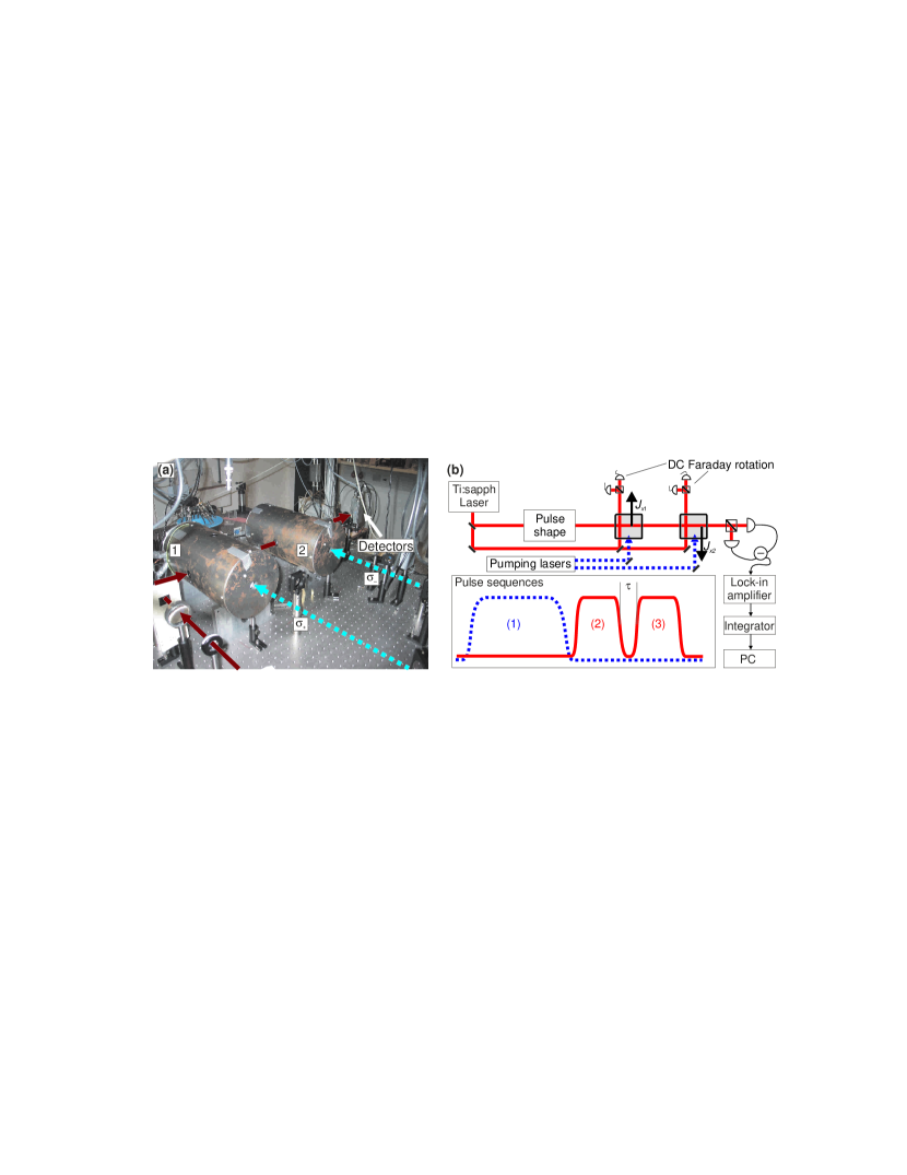
Figure 1: (a) A photographic view of the experimental setup. Atomic vapour cells are placed inside the cylindrical magnetic shields. The pumping beams are indicated with dashed arrows and the path of the entangling and verifying pulse is marked with the solid arrows. (b) A schematic view of the setup. The pulses reach a detection system measuring $\hat{S}_{y}(t)$. The photocurrent is sent to a lock-in amplifier which singles out the $\sin(\Omega t)$ and $\cos(\Omega t)$ parts. These are integrated and stored in a PC. The pulse sequence consists of (1) a 4ms pumping pulse, (2) a 2ms entangling pulse, a small delay $\tau=0.25\textrm{ms}$, and (3) a 2ms verifying pulse. In addition to the pumping lasers and the entangling and verifying pulse, a laser beam is sent through each sample to measure the magnitude $J_{x}$ of the macroscopic spins by Faraday rotation measurements.

In one measurement cycle the first step is to create the coherent spin state of the atomic samples. To this end we have two diffraction grating stabilized diode lasers, one at the 894nm D1 transition $6S_{1/2}\rightarrow 6P_{1/2}$ and one at the 852nm D2 transition $6S_{1/2}\rightarrow 6P_{3/2}$. We call these the optical pump and the repump, respectively. Both are sent through the first gas sample along the $x$-axis with $\sigma_{+}$ polarization, thus driving $\Delta m=+1$ transitions only. In the second gas sample the polarization is $\sigma_{-}$. The main pumping is done by the optical pump laser, which drives the atoms towards the $F=4$, $m_{F}=4$ state (for $\sigma_{+}$-polarization). This state will be unaffected by the optical pumping laser (a dark state) because of the absence of an $F=5$ state in the $6P_{1/2}$ multiplet. In the pumping process some of the atoms will decay into the $F=3$ ground state, which is why we need the repumping laser from this state to the $6P_{3/2}$ state to return them to the pumping cycle. Note that we can to some extent control the number of atoms in the $F=4$ ground state with the power of the repump laser. With this optical pumping scheme we can obtain spin polarization above 99% (measured by methods similar to [mors]). The pumping pulses last for 4ms and are shaped by Acousto Optical Modulators.

The atomic samples are now prepared in the CSS with anti-parallel macroscopic orientation. Next the off-resonant entangling pulse shaped by an Electro Optical Modulator of duration 2ms is sent through both cells to the $\hat{S}_{y}$ detection. The difference signal is fed into a lock-in amplifier and the result is two numbers $A_{1}$ and $B_{1}$ corresponding to the integrated ${\hat{J}}_{y1}^{\prime}+{\hat{J}}_{y2}^{\prime}$ and ${\hat{J}}_{z1}^{\prime}+{\hat{J}}_{z2}^{\prime}$ signals with an additional light contribution from the incoming $\hat{S}_{y}^{\mathrm{in}}(t)$. The entangling (and verifying) pulses have power of $P=4.5$mW and are blue detuned by 700MHz compared to the $6S_{1/2},F=4\rightarrow 6P_{3/2},F^{\prime}=5$ transition. They emerge from a Microlase Ti:sapphire laser which is pumped by an 8W Verdi laser.

After the entangling pulse is a short $\tau=0.25$ms delay before the verifying pulse is sent through the atoms. The entangling and verifying pulses have exactly the same shape and duration. The verifying pulse will again result in two numbers $A_{2}$ and $B_{2}$ stored in a PC. We now must predict the outcomes $A_{2}$ and $B_{2}$ based on $A_{1}$ and $B_{1}$ as described in section 3. In order to calculate the statistics properly we repeat the measurement cycle 10.000 times.

Measuring the Macroscopic Spin

In addition to the entanglement creation and verification we also measure the macroscopic value $J_{x}$ of the spin samples by sending linearly polarized light along the direction of optical pumping in both samples. This light experiences polarization rotation proportional to $J_{x}$. As already noted we have for small angles $\theta=S_{y}/2S_{x}$. We also know $S_{y}=aS_{x}J_{x}$ (for small angles, $S_{y}^{\mathrm{in}}$ is zero classically) when light is propagating along the $x$-direction. Holding these together we find (this holds for all angles)

$$\theta[\mathrm{rad}]=\frac{aJ_{x}}{2}=-\frac{\gamma\lambda^{2}J_{x}}{16\pi A_{\mathrm{eff}}\Delta}.$$ (37)

Instead of the beam cross section $A$ we need to use the effective cross section $A_{\mathrm{eff}}=6.0\mathrm{cm}^{2}$ which is such that the volume of the vapour cell is $V=A_{\mathrm{eff}}\cdot L$ where $L$ is the length traversed by the laser beam (we call it “effective” since the vapour cell is not exactly box like). We only measure polarization rotation from atoms inside the beam cross section (which does not fill the whole volume) and the equation must be scaled in order to count $J_{x}$ for all atoms (we have $J_{x}=J_{x}^{\textrm{in beam}}\cdot A_{\mathrm{eff}}/A$).

The DC Faraday rotation angle $\theta$ is a practical handle on the macroscopic spin size $J_{x}$ but we may in addition calculate a theoretical level for the projection noise to shot noise ratio $\kappa^{2}=\mathrm{PN/SN}$. Theoretically $\kappa^{2}=a^{2}J_{x}S_{x}T$ where again it is a question which cross section $A$ to insert in $a$. The entangling and verifying pulses do also not fill the entire vapour cell volume. We assume that the measurement results are not depending much in the real cross section for the following reason. If $A$ is small the interaction with the atoms inside the beam is stronger, but each atom will spend less time inside the beam leading to a correspondingly shorter effective interaction time $T$ (atoms are at room temperature and move in and out of the beam). If this simple consideration has some validity we may assume that the light fills the whole cell volume and the correct cross section to insert is the effective area $A_{\mathrm{eff}}$. Now this can be hold up against (37). Inserting $\lambda=852$nm, $\gamma=5$MHz and expressing the photon flux $\phi=2S_{x}$ in terms of probe power we may derive

$$\kappa^{2}_{\mathrm{theory}}=\frac{18.6\cdot P[\mathrm{mW}]\cdot T[\mathrm{ms}]\cdot\theta[\mathrm{deg}]}{\Delta[\mathrm{MHz}]}.$$ (38)

We remember the theory is a bit crude but we will see in Sec. 5 that the model holds pretty well.

5 Experimental Results

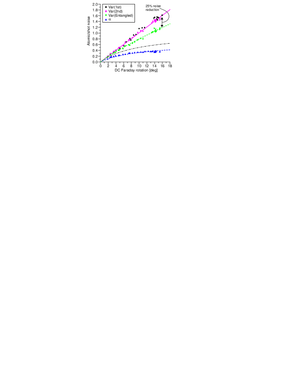
Figure 2: Atomic noise in units of shot noise as a function of atomic density (measured by DC Faraday rotation). Shot and electronics noise has been subtracted. Squares show the 1st pulse noise, circles the 2nd pulse noise. The linearity of these data is a finger print of the projection noise level which is then given by the solid line linear fit. Tip down triangles show the noise of the entangled states. Tip up triangles show the weight factor $\alpha$. The two dashed curves trough triangles is the model described in Eqs. (35) and (36) with $\beta=0.65$. The dash-dotted curve is the theoretically best for the triangles ($\beta=1$). Note that the states created by the first pulse measurements are really entangled states (according to the criterion (31)) since the noise is clearly below the PN. We observe up to 25% noise reduction. Note, entanglement is observed for low densities also with $\kappa^{2}<1$.

The experimental data is shown in Fig. 2, in the following we carefully explain the details of this graph.

The Projection Noise Level

The graph in Fig. 2 has on the abscissa the measured DC Faraday rotation angle which is proportional to $J_{x}$. The squares are the variances $\mathrm{Var}(A_{1})+\mathrm{Var}(B_{1})$ for the entangling pulses with shot noise (and electronics noise) subtracted. Also, the results are normalized to shot noise. The circles are the variances $\mathrm{Var}(A_{2})+\mathrm{Var}(B_{2})$ for the verifying pulses with the same normalization. According to Eq. (28) we have plotted the experimental ratio $\kappa^{2}=\mathrm{PN/SN}$ (the unity term in (28) is the subtracted shot noise). The linearity with $J_{x}$ confirms that we measure projection noise of atoms and not extra classical noise. We have roughly $\kappa^{2}_{\mathrm{exp}}=0.10\cdot\theta[\mathrm{deg}]$ which should be compared to the prediction (38) $\kappa^{2}_{\mathrm{theory}}=0.24\cdot\theta[\mathrm{deg}]$. The discrepancy is a little more than a factor of two but this is acceptable for our quite simple modeling. Note that the noise of the verifying pulse is the same as that of the entangling pulse. This is expected since we are performing a QND measurement. It is only when we remember the information given to us by the measurement results $A_{1}$ and $B_{1}$ that we can tell more about the state created by the entangling pulse.

Conditional Variances and Entanglement

The tip down triangles in Fig. 2 is the conditional variance $\mathrm{Var}(A_{2}|A_{1})+\mathrm{Var}(B_{2}|B_{1})$ normalized to shot noise and with shot and electronics noise subtracted. According to (31) we thus plot $\kappa^{2}(\mathrm{Var}(\hat{P}_{A1}^{\mathrm{ent}})+\mathrm{Var}(\hat{P}_{A2}^{\mathrm{ent}}))$. The fact that the points are lower than the straight line ($\kappa^{2}$) is a direct indication that the entanglement criterion (27) is fulfilled. For the higher densities the reduction is 25% but we note that entanglement is also observed for smaller densities with $\kappa^{2}<1$. The latter was impossible with the older methods applied in [nature]. The corresponding $\alpha$-parameters from the minimization procedure (29) are plotted in Fig. 2 with tip up triangles.

The expected entangled noise level in the ideal case is given by (33). This is drawn as the dash-dotted curve ($\kappa^{2}$ times $1/(1+\kappa^{2})$). We see the conditional variance lies higher than this curve and hence the entanglement is worse than expected. According to (34) we also would expect the $\alpha$-parameters to lie on the same dash-dotted curve in the ideal case. It is clearly not the case, the experimental $\alpha$-parameters are lower which indicates that the results $A_{1}$ and $B_{1}$ can not be trusted to as high a degree as expected.

Let us try to apply the simple decoherence model given by Eqs. (35) and (36). Taking the decoherence parameter $\beta=0.65$ we get the dashed lines in the figure. These match nicely the experimental data. We conclude that the simple decoherence model has some truth in it and we must accept that the entangled state created can only be verified to be around “65% as good” as expected in an ideal world.

Physical Decoherence Processes

Above we quantify the observed decoherence with the $\beta$-parameter. Here we comment on the physical grounds for the decoherence. A well known parameter for describing the decay of the transverse spin components $J_{y}$ and $J_{z}$ is the $T_{2}$-time defined by

$$\frac{\partial J_{i}}{\partial t}=-\frac{J_{i}}{T_{2}}$$ (39)

where $i=y,z$. We have studied the $T_{2}$-time extensively. A very good method for this is to create (by applying an RF-magnetic pulse) a displaced version of the coherent spin state with e.g. $\left<{\hat{J}}_{y}^{\prime}\right>\neq 0$. This non-zero mean value can be detected by our standard $\hat{S}_{y}$-detection method and the decay following (39) may be observed.

Our experience tells us that power broadening by the laser pulses combined with light assisted atomic collisions play the important role in the decoherence processes. For high densities and high optical powers we may find $T_{2}$ as low as 5ms. A fair guess for $\beta$ is an exponential decay over a typical time scale of 2ms (the time between the central parts of the entangling and verifying pulses). This yields $\beta\approx\exp(-2\mathrm{ms}/5\mathrm{ms})\approx 0.67$. This is not far from the observed $\beta$ but we should say here that the 5ms is a typical value not directly measured in the case of the data given in Fig. 2. It is our experience that the observed decoherence in the entanglement experiments is stronger than that expected from the processes mentioned above. This is indeed true for shorter pulses. We believe that the atomic motion in and out of the laser beam combined with inhomogeneous light/atom coupling due to the Doppler effect may also play a role, but we need further investigation to confirm this completely.

Conclusion of Experimental Results

To conclude the experimental section we emphasize that we have generated entangled states between distant atomic samples in the sense that each vapour cell sits in its own magnetic shield. The two shields can in principle be moved as far apart as is practical, our experiment was performed with a distance of 35cm. In the future we hope to extend this distance further. The noise reduction below the level set by separable states was measured up to 25%. This number is mainly limited by power broadening and light assisted collisional relaxation of the atomic spins. The decoherence is successfully modeled by a single parameter $\beta$. A much more elaborate theory on entanglement generation in presence of decoherence and losses exists [myart]. We should note, that the generated entangled states have random but known (based on $A_{1}$ and $B_{1}$) mean values. It is possible by applying RF-magnetic fields to shift the entangled states to having zero mean value while preserving the reduced variance. Experimental demonstration of such will be considered elsewhere.

6 Perspectives

We will now present a brief overview of some of the interesting applications in the field of quantum information of our reliable source of distant atomic entanglement.

Atomic Teleportation

Quantum teleportation was first proposed in 1993 [bennett] and the year after for the special case of continuous variables [vaidman]. Teleportation is extremely important since direct transport of physical states is often hindered by exponential decoherence. With quantum teleportation the information is cleanly separated into a classical part, which can be transmitted over arbitrary distances, and a quantum mechanical part, which only needs to interact locally.

A proposal for spin state teleportation was given in [Duan]. Three atomic samples are needed as shown in Fig. 3(a). Adjacent samples are oriented oppositely along the $x$-axis so that both collective measurements on cells 1 and 2 and on cells 1 and 3 will be regular entangling interactions as discussed earlier. Cells 1 and 3 are located at Alice’s site and cell 2 at Bob’s site. The goal is now to teleport an unknown state in cell 3 onto cell 2. First cells 1 and 2 are entangled giving the measurement results $(A_{1},B_{1})$. Next a pulse is sent through cells 1 and 3 and the measurement results $(A_{2},B_{2})$ are communicated classically to Bob. He can now by applying a rotation to his system based on the outcomes of the two measurements recreate the unknown state in his cell. This of course only works with perfect fidelity in the large interaction regime ($\kappa^{2}\gg 1$).

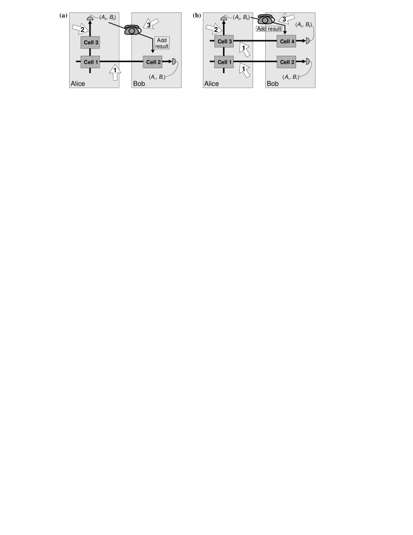
Figure 3: (a) Teleporting an unknown quantum state: first cells 1 and 2 are entangled. Then Alice sends a light pulse through cell 1 and the unknown quantum state in cell 3. The measurement results are communicated classically to Bob who by applying a displacement to his system based on the results of the two measurement recreates the unknown quantum state in his cell. (b) Entanglement swapping: the same procedure as in (a) but with two sets of entangled states initially. After a displacement based on the measurement results cells 2 and 4 are entangled even though they have never interacted directly.

Teleporting an Entangled State: Entanglement Swapping

As described in [royal] an entangled state can also be teleported using macroscopic samples of atoms. In this case Alice and Bob each have two samples (Fig. 3(b)). First each one of Alice’s samples are entangled with one of Bob’s. Then a pulse of light is sent through Alice’s two samples making it an entangled state. Alice now sends the result of a measurement on this last entangling pulse to Bob. Using this and the results of the two primary entangling pulses he can displace one of his states. This entangles his two samples without ever bringing the two into direct contact. Had Alice shifted one of her spin states prior to creating the entanglement between her two cells the exact same protocol would allow Bob to recover this shift in his cells. This allows for secret quantum communication.

Light to Atom Teleportation: Quantum Memory

With an entangled source of atoms an unknown state of light can also be teleported onto this [kuzmich]. Assume we have two atomic samples with $\hat{J}_{y1}+\hat{J}_{y2}=0$ and $\hat{J}_{z1}+\hat{J}_{z2}=0$, i.e. a perfect EPR-entangled state. The protocol is simpler without rotating spins but also works with. As can be seen from Eq. (6) $\hat{J}_{z}$ is mapped onto $\hat{S}_{y}$ when light propagating along the $z$ axis is sent through an atomic sample. If light is sent through the first atomic sample and subsequently detected the measurement result can be fed back into $\hat{J}_{z2}$ such that the original atomic variables exactly cancel. $\hat{S}_{y}$ has now been mapped perfectly onto $\hat{J}_{z2}$. Another effect of the light pulse is seen from Eq. (8). $\hat{S}_{z}$ is mapped onto $\hat{J}_{y1}$. If the transverse spins of sample 1 are rotated $90^{\circ}$ and a new strong light pulse ($\kappa^{2}\gg 1$) is sent through this sample $\hat{J}_{y1}^{\mathrm{out}}$ is measured. This result can be fed back onto $\hat{J}_{y2}$ in such a way that the two original $\hat{J}_{y}$’s cancel. $\hat{S}_{z}$ is now stored in $\hat{J}_{y2}$ and the teleportation is complete. This process could also be reversed so that an unknown atomic state is mapped onto a light pulse via two EPR-entangled light beams. This shows that macroscopic samples of atoms offers a very feasible protocol for complete quantum memory.

7 Summary and Conclusion

We have presented the first experimental realization of distant atomic entanglement in the sense that the two atomic systems are placed in separate environments, thus enabling entanglement between system separated by arbitrary distances. Given the abundance of available quantum information protocols for this type of continuous variable atomic system the importance of this achievement is evident. Although quantum teleportation of atomic states has been achieved recently [wineland, blatt] none of these approaches display directly scalable distance between the unknown quantum state and the target system. Our system must therefore be considered an important candidate for achieving the long standing goal of high fidelity transfer of atomic states over great distances upon which many of the proposed technical applications of entanglement and teleportation critically depend. The existence of several quantum information protocols for our physical system is based on the simplicity of the interaction between light and atoms as expressed by Eqs. (25a-d).

Acknowledgments

This work is supported by the Danish National Research Foundation and the European Union through the grant QUICOV.

distantdistant