Probabilistic Quantum Control Via Indirect Measurement

Abstract

The most basic scenario of quantum control involves the organized manipulation of pure dynamical states of the system by means of unitary transformations. Recently, Vilela Mendes and Mank’o have shown that the conditions for controllability on the state space become less restrictive if unitary control operations may be supplemented by projective measurement. The present work builds on this idea, introducing the additional element of indirect measurement to achieve a kind of remote control. The target system that is to be remotely controlled is first entangled with another identical system, called the control system. The control system is then subjected to unitary transformations plus projective measurement. As anticipated by Schrödinger, such control via entanglement is necessarily probabilistic in nature. On the other hand, under appropriate conditions the remote-control scenario offers the special advantages of robustness against decoherence and a greater repertoire of unitary transformations. Simulations carried out for a two-level system demonstrate that, with optimization of control parameters, a substantial gain in the population of reachable states can be realized.

I Introduction

The conditions under which a quantum-mechanical system is controllable and the degree to which control is possible are issues of considerable theoretical and practical importance. Many different definitions of controllability are currently in play. Let us suppose the time-development of the system is described by a Schrödinger equation (with $\hbar=1$)

$$i\frac{d}{dt}|\psi(t)\rangle=\left[H_{o}+\sum_{n=1}^{r}f_{n}(t)H_{n}\right]|\psi(t)\rangle\,,$$ (1)

where the $f_{n}(t)$ are independent, bounded, measurable control functions. The most common notion of controllability is pure-state controllability schi , taken to mean that starting in any given pure state $|\psi_{0}=|\psi(t_{0})\rangle$, there exists a set of control functions $f_{n}(t)$ such that any pure final state $|\psi_{f}\rangle=|\psi(t_{f})\rangle$ can be reached at some later time $t_{f}>t_{i}$. This is equivalent to saying that there exists a set of control functions $f_{n}(t)$, a time $t_{f}>t_{0}$, and a unitary operator $U(t)$ satisfying

$$i{d\over dt}U(t)=\left[H_{o}+\sum_{n=1}^{r}f_{n}(t)H_{n}\right]U(t)\,,$$ (2)

such that $U(t_{0})|\psi_{0}\rangle=|\psi_{0}\rangle$ and $U(t_{f})|\psi_{0}\rangle=|\psi_{f}\rangle$. A stronger condition is complete controllability, in the sense that any unitary operator $U$ is dynamically accessible from the identity operator.

The most incisive results are available for the restricted, but practically important, case of a system with a finite number of energy levels, more precisely, a system whose eigenstates span a Hilbert space with finite dimension $N$. In particular, a necessary and sufficient condition for pure-state controllability schi is that the dynamical Lie group $G({\cal A})$ generated by the set of operators $\{iH_{0},iH_{1},\ldots iH_{r}\}$ is equal to $U(N)$, $SU(N)$, or (if $N$ is even) either $Sp(N/2)$ or $Sp(N/2)\times U(1)$. It may be shown that these conditions can only be satisfied if the dynamical Lie algebra of the system is $u(N)$, $su(N)$, or (if $N$ is even) either $sp(N/2)$ or $sp(N/2)\oplus U(1)$. Complete controllability of the $N$-level problem is naturally more demanding: It is necessary and sufficient that $G({\cal A})$ coincide with the largest of the groups listed, namely $U(N)$.

We note that fundamental theorems on controllability were established for a more general class of quantum systems at the very beginning of the subject of quantum control huang ; clark02 ; clark03 . This class includes continuous systems with unbounded observables (e.g., position, momentum, kinetic energy), whose states span an infinite-dimensional Hilbert space. The domain problems were dealt with by assuming the existence of an analytical domain in the sense of Nelson nelson , and available geometric methods for finite-dimensional bilinear control systems brockett ; sussmann1 ; sussmann2 ; kunita were adapted to derive controllability results in terms of certain Lie algebras. In fact, theorems commonly stated for finite-level systems may be extracted as special cases of the results of Ref. huang .

The objective of this paper is expand the scope of control beyond the implementation of unitary operators, exploiting the phenomenon of entanglement and the option to carry out measurements on the given system (or its surrogate). In the interest of transparency, we shall avoid troublesome domain problems by focusing on a quantum system described in a state space of finite dimension $N$.

We take as a starting point the recent result of Vilela Mendes and Man’ko mendes establishing that in some situations, a nonunitarily controllable system can be controlled by the joint action of projective measurement plus unitary evolution. More precisely:

Theorem: For a specified target state $|\psi_{f}\rangle$, there exists a family of observables $M[|\psi_{f}\rangle]$ such that measurement of any one of them on an arbitrary initial state $|\psi_{0}\rangle$, followed by unitary evolution, leads to $|\psi_{f}\rangle$ if $G({\cal A})$ is either $O(N)$ or $Sp(N/2)$.

As pointed out in Ref. mendes , the system is already pure-state controllable if $G({\cal A})=Sp(N/2)$, but it still might be more efficient to use the measurement/evolution strategy. Also, if both the initial and final states are fixed, pure-state controllability may be achieved with this strategy even if $G({\cal A})$ is a much smaller subgroups of $U(N)$ than $O(N)$ or $Sp(N/2)$.

Thus, the conditions required for controllability are weakened if unitary control is supplemented by projective measurement. However, when the measurement is performed on a given observable of the system, the possible outcomes are necessarily restricted to the set of eigenstates of this observable.

The present work aims to overcome this limitation by extending the hybrid measurement/unitary approach to control a step further, exploring the additional prospects opened by performing the measurement on an entangled partner of the system in question (cf. Ref. lloyd ). The basic scheme is introduced in Sec. II. As anticipated by Schrödinger schr in 1935, a salient feature of this exploitation of entanglement is that the “remote control” so attempted can no longer absolute, but is instead probabilistic in character. Nevertheless, an enlargement of the reachable set of states can be achieved. Alternative algebraic and geometric descriptions of the proposed control scheme are presented in Sec. III. In Sec. IV, we illustrate the possibilities opened by the remote-control strategy for the simple case of a two-level system ($N=2$) as realized, for example, by a Pauli spin 1/2. The efficacy of the method, measured by the number of reachable final states and the probability of a successful outcome, is tested in a simulation in which adjustable control parameters are optimized to minimize the distance of the actual state from the desired final state. In Sec. V we consider the effects of decoherence within the remote-control scenario. As usual, the directly controlled system suffers from decoherence due to its environment, whereas the remotely controlled target system, kept isolated from its surroundings, remains immune. We conclude in Sec. VI with some remarks on the genesis of the idea proposed here, and on its further development.

II Control via Entanglement

The proposed control scheme – control via indirect projective measurement – involves three basic steps. Two systems are involved: (i) the target $N$-level system, which we wish to move by means of indirect influences into a pre-selected final state and (ii) the control system, an identical, entangled partner of the target system which is directly steered or shoved by control operations from the available repertoire. It is supposed that the target system is initially in a pure state

$$|\psi^{(\rm t)}\rangle=\sum_{i=1}^{N}c_{i}|e_{i}^{(\rm t)}\rangle\,,$$ (3)

expressed in a convenient basis $\{|e_{i}^{(\rm t)}\rangle\}$. Likewise, the control system is initially in a pure state $|\psi^{(\rm c)}\rangle$ similarly expressed in its own state space.

First, we entangle the target system with the control system, e.g. by means of a non-local two qubit operation. The combined system undergoes the change

$$|{\psi}^{(\rm t)}\rangle\otimes|{\psi}^{(\rm c)}\rangle=\sum_{i=1}^{N}c_{i}|e_{i}^{(\rm t)}\rangle\otimes\sum_{l=1}^{N}b_{l}|e_{l}^{(\rm c)}\rangle\ \stackrel{{\scriptstyle\cal E}}{{\longrightarrow}}|\chi\rangle=\sum_{i=1}^{N}a_{i}|e_{i}^{(\rm t)}\rangle\,|e_{i}^{(\rm c)}\rangle\,,$$ (4)

where ${\cal E}$ symbolizes entanglement and we suppress the tensor product notation in the third member. In the density-matrix formulation, the partial density matrix of the target system, obtained by tracing over the control system, undergoes the transformation

$$(\rho^{(\rm t)})_{ij}=a_{i}a^{*}_{j}|e_{i}^{(\rm t)}\rangle\langle e_{j}^{(\rm t)}|\stackrel{{\scriptstyle\cal E}}{{\longrightarrow}}(\rho^{(\rm t)})_{ij}=|a_{i}|^{2}|e_{i}^{(\rm t)}\rangle\langle e_{j}^{(\rm t)}|\delta_{ij}\,.$$ (5)

Second, one of the available unitary transformations $U(t)$ is applied to the control system thus:

$$|\chi^{\prime}\rangle=\sum_{i,j=1}^{N}U_{ji}a_{i}|e_{i}^{(\rm t)}\rangle\,|e_{j}^{(\rm c)}\rangle\,.$$ (6)

While $\rho^{(\rm t)}$ remains unaffected, the partial density matrix $\rho^{(\rm c)}$ of the control system begins a forced evolution according to

$$(\rho^{(\rm c)})_{ij}=|a_{i}|^{2}|e_{i}^{(\rm c)}\rangle\langle e_{j}^{(\rm c)}|\delta_{ij}\rightarrow({\rho^{(\rm c)}}^{\prime})_{ij}=\sum_{k=1}^{N}U_{ik}|a_{k}|^{2}U_{kj}^{*}|e_{i}^{(\rm c)}\rangle\langle e_{j}^{(\rm c)}|\,.$$ (7)

In the third and final step, a projective measurement is performed on the control system for a selected observable $X$. Without loss of generality, we may assume that the basis $\{|e_{i}^{(\rm c)}\rangle\}$ in the state space of the control system is an eigenbasis of the chosen observable, which may then be expressed as

$$X=\sum_{n=1}^{N}x_{n}|e_{n}^{(\rm c)}\rangle\langle e_{n}^{(\rm c)}|\,.$$ (8)

The measurement will then yield the eigenvalue $x_{m}$ of $X$ with probability

$$P_{m}=\sum_{i=1}^{N}U_{mi}|a_{i}|^{2}U_{im}^{*}\,,$$ (9)

leaving the combined system in a state that is no longer entangled, namely

$$|\chi_{m}^{\prime\prime}\rangle=\frac{1}{\sqrt{P_{m}}}\sum_{k=1}^{N}U_{mk}a_{k}|e_{k}^{(\rm t)}\rangle\otimes|e_{m}^{(\rm c)}\,\rangle\,.$$ (10)

It is seen that the final state of the target system is in general a superposition of eigenstates of the observable $X$, rather than the particular eigenstate corresponding to the result of measurement, as it would be in a simple direct projective measurement. Furthermore, there are $N(>1)$ possible results of the three-step control procedure, which therefore assumes a probabilistic character. As we shall see, the advantage of certainty of outcome is traded for a potentially expanded range of control. Another positive aspect of remote control is that it can overcome the limitation of unitary control to transformations of the state of the target system within a restricted equivalence class determined by the set of eigenvalues of the initial density matrix schi .

III Algebraic and Geometric Descriptions of Indirect Control

III.1 Algebraic Treatment

The total effect of the indirect control scheme on the target system can be represented in terms of a set of $N$ diagonal matrices $\Upsilon_{m}=\left(U_{ml}\delta_{ln}\right)$ representing Kraus operators, one for each of the $N$ possible results of the measurement performed on the control system. Due the unpredictability of the final state, the property of controllability, as strictly defined, does not apply to the target system.

This situation contrasts with what is found in the theory of universal quantum interfaces developed in Ref. landahl , where similar schemes involving remote control are formalized, but with broader intent within the contexts of quantum computation and quantum communication. In that work, the target system is shown to be both controllable and observable through control and observation of the control bit to which it is coupled. The main distinction between the two approaches is the following. In Ref. landahl , the control and target systems remain in close proximity and the interaction between them can have indefinite duration, whereas in the remote-control scenario envisioned here, the systems are in transient interaction, and then separate from one another. In some circumstances, the disjunction of the two systems may prove desirable or advantageous.

Controllability being moot, our consideration turns to reachable sets of the target system. It is easily seen that if the control system is controllable, then every state of the target system is reachable. Every unitary transformation $U$ of the target system is available for temporal manipulation of the control system. To each of these there correspond $N$ non-unitary transformations $\Upsilon_{m}$, and the mapping between $U$ and each of the $\Upsilon_{m}$ is one-to-one. Hence, every state of the target system is reachable.

If the control system is not controllable, then every state of the target system may or may not be reachable. To illustrate this possibility, consider the case in which both the control and target systems are spin-$1/2$ particles. Let the unitary transformations available for application be specified by

$$U(\theta,\phi)=\left(\begin{array}[]{ccc}\cos(\theta/2)&-\sin(\theta/2)e^{i\phi}\\ \sin(\theta/2)&\cos(\theta/2)e^{i\phi}\end{array}\right)\,,$$ (11)

where $0\leq\phi<\pi$ and $0\leq\theta\leq\pi/2$. In this case, the set of the states reachable from an initial state on the equator of the Bloch sphere covers only two quadrants of the Bloch sphere.

Let us apply these transformation to a control system that is maximally entangled with the target system, and then perform a measurement on the spin component $\sigma_{z}$ of the control system. The available transformations are then expanded to

$$\Upsilon_{1}(\theta,\phi)=\left(\begin{array}[]{cc}\cos(\theta/2)&0\\ 0&-\sin(\theta/2)e^{i\phi}\end{array}\right)\,,\qquad\Upsilon_{2}(\theta,\phi)=\left(\begin{array}[]{cc}\sin(\theta/2)&0\\ 0&\cos(\theta/2)e^{i\phi}\end{array}\right)\,.$$ (12)

Thus, the reachable set for the target system is the whole Bloch sphere, even if the set reachable by applying only the specified $U$ transformations is just two quadrants. We note that the assumed condition of maximal entanglement simplifies the proof but is not essential. This possibility for enlargement of the reachable set is illustrated in the optimization problem solved in the next section.

Sequential application of the probabilistic remote-control scheme is not in general effective in further extension of the range of control. The $\Upsilon_{m}$ matrices are diagonal and necessarily commute with one another; consequently, the advantages of a Lie algebra do not apply. Unlike unitary operators, Kraus operators are not guaranteed the property that they can be combined to give new directions of control in the state space viola .

Finally, if $\Upsilon_{m}$ operations are combined with unitary operations on the target system, the commutativity is lifted and the repertoire of available transformations on the target system is enlarged. Again we chose a two-level example to illustrate the point. Suppose the only available quantum gate for the system is the Hadamard gate

$$U_{H}=\frac{1}{\sqrt{2}}\left[\begin{array}[]{cc}1&1\\ 1&-1\end{array}\right]\,.$$ (13)

Then upon implementing the probabilistic remote-control scheme for this target system (involving entanglement, application of the Hadamard gate on the control qubit, and projective measurement), we obtain an additional gate

$$\Upsilon_{2}=Z=\left[\begin{array}[]{cc}1&0\\ 0&-1\end{array}\right]\,.$$ (14)

By successive applications of $U_{H}$ and $Z$ we further extend the set of reachable states. In this case it happens $\Upsilon_{1}=I$ and $\Upsilon_{2}=Z$ are both unitary, but it will not generally be the case that all the $\Upsilon_{m}$ are unitary. It is interesting to note that the probabilistic character of the control scheme can be overcome by applying unitary transformations on the target system so as to feed back the indirect measurement results, as proposed in Ref. viola .

III.2 Geometric Treatment

Again for the sake of simplicity and clarity, we consider a two-level system ($N=2$). Physically, the system might be a single Pauli spin-1/2 or a two-level atom, having energy eigenstates denoted $|0\rangle$ and $|1\rangle$.

The geometric description is based on the coherent-vector (or Bloch-vector) picture of quantum dynamics alicki ; emma . The coherent vector $\bf v$ can represent a pure state on the Bloch sphere as well as a mixed state lying in the interior of the sphere. Its magnitude, or length, is defined by $\|{\bf v}\|=({\rm tr}{\rho}^{2}-1/2)^{1/2}$, and its Cartesian components by $v_{x}=2^{-1/2}{\rm tr}(\rho\sigma_{x})$, $v_{y}=2^{-1/2}{\rm tr}(\rho\sigma_{y})$, and $v_{z}=2^{-1/2}{\rm tr}(\rho\sigma_{z})$. Whether it refers to an entangled or non-entangled quantum system, the coherent vector $\bf v$ evolves with time according to the following rules.

• The coherent vector may shrink in magnitude, i.e., contract to a shell of smaller radius, if and only if the system becomes entangled. The tip of the vector traces a continuous path, namely a line passing through the initial position and perpendicular to the axis that connects the einselected states pente [see Fig. 1(a)]. Either premeasurement pente or decoherence will drive the coherent vector in this manner, because both these processes imply entanglement.

• A unitary transformation leaves ${\rm tr}{\rho}^{2}$ invariant and hence does not change the magnitude of the coherent vector $\bf v$. Accordingly, a unitary transformation can only rotate $\bf v$ on the shell of radius equal to $\|{\bf v}\|$ [see Fig. 1(b)]. The effect of the rotation is independent of the magnitude of the vector.

• A mixed state may become pure if the entangled state becomes disentangled and the bipartite system becomes separable. This can occur through projective measurement on one of the two systems. Both of the systems are purified, but not in a deterministic manner. The possible final states depend on the observable that is measured and on the entangled state. Figure 1(c) gives a simple example in which the projective measurement is made on an observable whose eigenstates coincide with the Schmidt basis of the measured system.

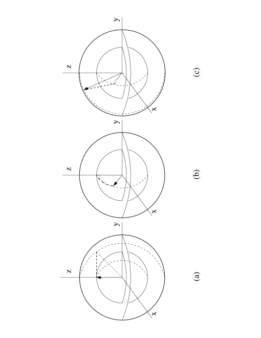
Figure 1: Coherent-vector representation of quantum dynamics for a two-level system. (a) The effect of entanglement on a pure state. (b) Unitary transformation of a mixed state. (c) Projective measurement on either system of an entangled pair. In each operation, the initial vector [final vector] is drawn as an arrow with a white [black] head.

Probabilistic, indirect quantum control, as introduced in Sec. II, involves all three of these operations. The geometric description of this process is illustrated in Fig. 2 for the $N=2$ case (which is actually the only nontrivial case that one can draw.) Reiterating, the scheme is to:

• Entangle the target system with the control system. This causes shrinkage of the coherent vectors of both systems [Fig. 2(a)].

• Apply a unitary transformation to the control system. The coherent vector ${\bf v}^{({\rm c})}$ of the control system rotates without change of magnitude, while the coherent vector ${\bf v}^{({\rm t})}$ of the target system is unaffected by the transformation [Fig. 2(b)].

• Make a projective measurement on the control system. The final coherent vectors are not determined. One has either ${\bf v}_{1}^{({\rm c})}$ or ${\bf v}_{2}^{({\rm c})}$ for the control system, ${\bf v}_{1}^{({\rm t})}$ or ${\bf v}_{2}^{({\rm t})}$ for the target [Fig. 2(c)]. The initial and final coherent vectors obey a set of angle rules; in particular

  $$\angle\left({\bf v}^{({\rm c})},{\bf v}^{({\rm t})}\right) = \angle\left({\bf v}^{({\rm c})},{\bf v}_{1}^{({\rm c})}\right)\,,\angle\left({\bf v}^{({\rm c})},{\bf v}^{({\rm t})}\right)=\pi-\angle\left({\bf v}^{({\rm c})},{\bf v}_{2}^{({\rm c})}\right)\,,$$

  $$\angle\left({\bf v}^{({\rm c})}_{1},{\bf v}^{({\rm t})}_{1}\right) = \angle\left({\bf v}^{({\rm t})},{\bf v}_{1}^{({\rm t})}\right)\,,\qquad\angle\left({\bf v}^{({\rm c})}_{2},{\bf v}^{({\rm t})}_{2}\right)=\pi-\angle\left({\bf v}^{({\rm t})},{\bf v}_{2}^{({\rm t})}\right)\,.$$ (15)

  Also, $\angle({\bf v}^{({\rm c})}_{1},{\bf v}^{({\rm c})}_{2})=\pi$, while $\angle({\bf v}^{({\rm t})}_{1},{\bf v}^{({\rm t})}_{2})$ depends on the initial state of the target system and the unitary transformation applied to the control system. In the special case where the two systems are maximally entangled then $\angle({\bf v}^{({\rm t})}_{1},{\bf v}^{({\rm t})}_{2})=\pi$.

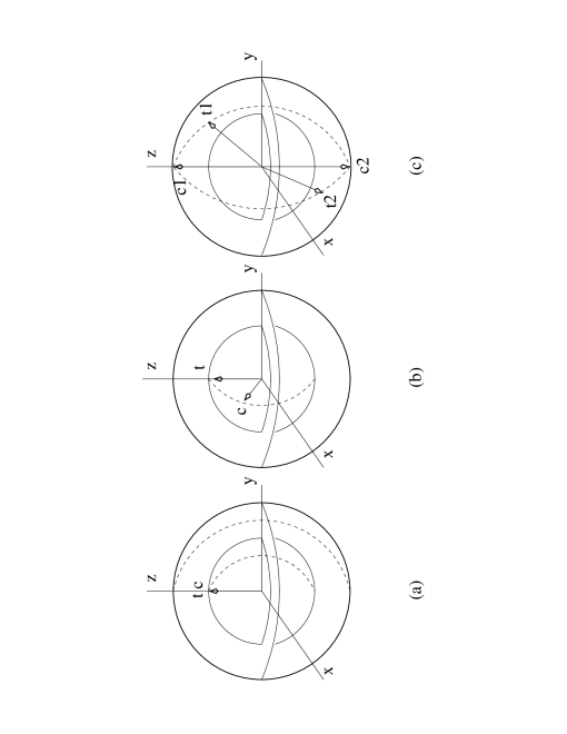
Figure 2: (a) Control and target system become entangled. (b) A unitary transformation is applied to the control system. (c) A projective measurement is performed on the control system.

With exclusive use of unitary transformations to control a system, the coherent vector is rigorously confined to the shell of the Bloch sphere. Probabilistic remote quantum control permits the coherent vector to move to the interior of the sphere as well, thereby opening new pathways to the desired final state.

IV Optimized probabilistic control: A simulation

The benefits (and drawbacks) of the probabilistic remote-control process are exemplified in a problem drawn from nuclear magnetic resonance. If there is a constant magnetic field of strength $B_{0}$ present along the $z$-axis, the Hamiltonian of a spin-1/2 particle is $H_{o}=\omega\sigma_{z}=\omega Z$, and the time evolution operator for the system is given by

$$U_{0}(t)=\left(\begin{array}[]{cc}e^{-i\omega t}&0\\ 0&e^{i\omega t}\end{array}\right)\,.$$ (16)

If a resonant magnetic field $(B_{x},B_{y})$ is also applied in the $x-y$ plane, we have an additional time-dependent gate

$$U_{1}(t)=\left(\begin{array}[]{cc}\cos(g\ t)&-i\ \sin(g\ t)\\ -i\ \sin(g\ t)&\cos(g\ t)\end{array}\right)\,.$$ (17)

Suppose we wish to reach a particular final state at the exact time $T$, by applying $U_{0}(T/2)$ and then $U_{1}(T/2)$. The parameters available for adjustment (“optimization”) are the field strengths $B_{0}$, $B_{x}$, and $B_{y}$, or more precisely $\omega$ and the coupling constant $g$. Here we note the precedent set by Ref. emma in organizing pure-state control of a two-level quantum system within the geometric intepretation on the Bloch sphere.

Simulations were performed to test the efficacy of two different control schemes, namely unitary control alone and the probabilistic remote-control scenario. A hundred random pairs of initial states were chosen and simulations were performed for both control schemes. With the initial time at 0, the numerical experiment was repeated for ten different final times $T$, keeping the adjustable parameters within the ranges $0\leq g\leq 2\pi$ and $0\leq\omega\leq 2\pi$. The two relevant performance measures are the fraction of final states successfully reached and the overall probability of reaching the final state of a pair. The results of averaging over all simulations are shown in Table I. As might be expected, the fraction of target states successfully reached is significantly larger , more than double when the indirect-measurement protocol is implemented. However, this advantage is compensated by the probabilistic nature of the remote-control process, such that the overall success rates for the two methods are similar.

Table I. Comparison of probabilistic remote control with pure unitary control, for a spin-1/2 system

Control	Number of	Target final	Net Probability
protocol	pairs tested	states reached	of success
Unitary	100	$2.4\pm 0.4$	$0.024\pm 0.004$
Remote	100	$6.6\pm 0.5$	$0.0345\pm 0.0012$

V Role of decoherence

Suppose that we entangle a pair of identical (sub)systems such that combined system is described by the state vector $|\psi\rangle$. Now, arrange that the two subsystems become separated, such that the target system, which is to be remote-controlled, is kept isolated from the environment, while the control system remains exposed in the laboratory, where we can perform unitary operations or measurements upon it. The control system soon interacts with the laboratory environment and becomes entangled with it; schematically,

$$|\psi\rangle=\sum_{i=1}^{N}a_{i}|e_{i}^{({\rm t})}\rangle\,|e_{i}^{({\rm c})}\rangle\otimes|{\rm env}\rangle\stackrel{{\scriptstyle{\cal E}}}{{\rightarrow}}|\psi\rangle=\sum_{i=1}^{N}a_{i}|e_{i}^{({\rm t})}\rangle\,|e_{i}^{({\rm c})}\rangle\,|{\bf\epsilon}_{i}\rangle\,,$$ (18)

where ${|{\bf\epsilon}_{i}\rangle}$ is a basis for the environment.

The entanglement between the target and control system is not affected by the presence of the environment yu , and the statistical properties of the target system remain the same, i.e.,

$$(\rho^{({\rm t})})_{ij}=\sum_{a=1}^{N}|a_{i}|^{2}|e_{i}^{({\rm t})}\rangle\langle e_{i}^{({\rm t})}|\delta_{ij}\,.$$ (19)

Following the remote-control scenario, we next apply a unitary transformation on the control system, to obtain

$$|\psi^{\prime}\rangle=\sum_{i,j=1}^{N}U_{ji}a_{i}|e_{i}^{({\rm t})}\rangle\,|e_{j}^{({\rm c})}\rangle\,|{\bf\epsilon}_{i}\rangle\,.$$ (20)

However, the environment is still present and becomes entangled with the new state of the control system:

$$|\psi^{\prime\prime}\rangle=\sum_{i,j=1}^{N}U_{ji}a_{i}|e_{i}^{({\rm t})}\rangle\,|e_{j}^{({\rm c})}\rangle\,|{\bf\epsilon}_{j}\rangle\,.$$ (21)

Finally, a projective measurement is performed on the control system, yielding

$$|\psi^{\prime\prime\prime}\rangle=\frac{1}{\sqrt{P_{m}}}\sum_{i=1}^{N}a_{i}U_{im}|e_{i}^{({\rm t})}\rangle\,|e_{m}^{({\rm c})}\rangle\,|{\bf\epsilon}_{m}\rangle=\frac{1}{\sqrt{P_{m}}}\sum_{i=1}^{N}a_{i}U_{im}|e_{i}^{({\rm t})}\rangle\otimes|e_{m}^{({\rm c})}\rangle\,|{\bf\epsilon}_{m}\rangle\,.$$ (22)

We observe that the same results are obtained for the target system as in the case where the environment is absent, whereas the control system feels the effects of decoherence.

VI Summary and prospects: Remote control on entangled pairs

Taking inspiration from quantum teleportation bennett and from prior work of Vilela-Mendes and Man’ko mendes in which unitary control is supplemented by projective measurement, we have introduced a strategy for indirect control (“remote control”) of a target system through projective measurement on its entangled partner. We have thereby contributed to an ongoing unification of concepts and mathematical techniques developed in the fields of quantum control clark02 ; clark03 and quantum information theory nielsen . The integration of these two thrusts began in 1995 with Lloyd’s demonstration lloyd2 that “almost any quantum logic gate is universal” – shorthand for the fact that universality in quantum computation can be achieved by repeated application of almost any two-level gate and a single-qubit gate. The proof of this statement rests on Lie-algebraic arguments that have long been a staple of geometric control theory.

Reversing the flow of ideas, we have exploited entanglement together with the option of projective measurement to enlarge the scope of quantum control beyond what is attainable with unitary transformations on system states. Under the remote-control protocol, some states that were unreachable via simple unitary control now become reachable. However, this advantage is tempered by the fact that the outcome of the final measurement operation is necessarily probabilistic, i.e., the outcome of remote control is described by a probability distribution over a set of quantum states.

Our attention here has been focused on the advantages that probabilistic control via indirect measurement may offer in the manipulation of a system occupying a single, initially pure quantum state. As is evident, the idea may be extended to initial states of subsystems of a larger system, which in general are not pure and must be represented as density matrices.

Let the target system be an entangled bipartite system $({\rm t}_{a},{\rm t}_{b})$ described by

$$|\psi^{(t)}\rangle=\sum_{i=1}^{N}a_{i}|e_{i}^{({\rm t}_{a})}\rangle|e_{i}^{({\rm t}_{b})}\rangle\,.$$ (23)

The degree of entanglement of the system in this state may be quantified in terms of von Neumann entropy of the subsystem, or more simply the Schmidt number nielsen . Whatever appropriate measure is chosen, it cannot be changed by applying a unitary transformation on either of the two subsystems. However, the same is not true for the transformation accomplished by remote control, which, for example, is capable of changing the Schmidt number of the bipartite system as we go from

$$|\chi\rangle=\sum_{i=1}^{N}a_{i}|e_{i}^{({\rm t}_{a})}\rangle|e_{i}^{({\rm t}_{b})}\rangle|e_{i}^{({\rm c})}\rangle$$ (24)

to

$$|\chi^{\prime}\rangle=\sum_{i,j=1}^{N}a_{i}U_{ji}|e_{i}^{({\rm t}_{a})}\rangle|e_{i}^{({\rm t}_{b})}\rangle|e_{j}^{({\rm c})}\rangle$$ (25)

to

$$|\chi^{\prime\prime}\rangle = \frac{1}{\sqrt{P_{m}}}\sum_{i=1}^{N}a_{i}U_{mi}|e_{i}^{({\rm t}_{a})}\rangle|e_{i}^{({\rm t}_{b})}\rangle|e_{m}^{({\rm c})}\rangle$$ (26)

$$= \frac{1}{\sqrt{P_{m}}}\sum_{i}a_{i}U_{mi}|e_{i}^{({\rm t}_{a})}\rangle|e_{i}^{({\rm t}_{b})}\rangle\otimes|e_{m}^{({\rm c})}\rangle\,.$$

In future work, the scheme proposed here will be applied to systems that are entangled with many degrees of freedom. In pursuing such an investigation, one would like to determine the extent to which non-unitary control operations can be used to counteract undesirable effects arising from interactions between the system and its environment.

References

- (1) S. G. Schirmer, A. I. Solomon and J. V. Leahy, J. Phys. A: Math. Gen. 35, 8551 (2002).
- (2) G. M. Huang, T. J. Tarn, and J. W. Clark, J. Math. Phys. 24, 2608 (1983).
- (3) J. W. Clark, D. G. Lucarelli, and T. J. Tarn, Int. J. Mod. Phys. B17, 5397 (2003).
- (4) J. W. Clark, T. J. Tarn, and D. G. Lucarelli, Proceedings of the 2003 International Conference “Physics and Control”, edited by A. L. Fradkov and A. N. Churilov, IEEE Catalog No. 03EX708C (2003).
- (5) E. Nelson, Ann. Math. 70, 572 (1959).
- (6) R. W. Brockett, Proc. IEEE 64, 61 (1976).
- (7) H. Sussmann and V. Jurdjevic, J. Diff. Eq. 12, 95 (1972).
- (8) V. Jurdjevic and H. Sussmann, J. Diff. Eq. 12, 313 (1972).
- (9) H. Kunita, Appl. Math. Optim. 5, 89 (1979).
- (10) R. Vilela Mendes and V. I. Man’ko, Phys. Rev. A 67, 053404 (2003).
- (11) S. Lloyd, Phys. Rev. A 62, 022108 (2000).
- (12) E. Schrödinger, Proc. Cambridge Philos. Soc. 31, 555 (1935).
- (13) S. Lloyd, A. J. Landahl and Jean-Jacques E. Slotine, Phys. Rev. A, 69, 012305 (2004).
- (14) S. Lloyd and L. Viola, Phys. Rev. A 65, 010101 (2001).
- (15) R. Alicki and K. Lendi, Quantum Dynamical Semigroups and Applications (Springer-Verlag, Berlin, 1987).
- (16) A. Emmanouilidou, X.-G. Zhao, P. Ao, and Q. Niu, Phys. Rev. Lett. 85, 1626 (2000).
- (17) W. H. Zurek, Rev. Mod. Phys. 75, 715 (2003)
- (18) T. Yu and J. H. Eberly, Phys. Rev. B 68, 165322 (2003).
- (19) C. H. Bennett, G. Brassard, C. Crépeau, R. Jozsa, A. Peres, and W. K. Wootters, Phys. Rev. Lett. 70, 1895 (1993).
- (20) M. A. Nielsen and I. L. Chuang, Quantum Computation and Quantum Information (Cambridge University Press, Cambridge, 2000).
- (21) S. Lloyd, Phys. Rev. Lett. 75, 346 (1995).