Fault-Tolerant Quantum Dynamical Decoupling

Abstract

Dynamical decoupling pulse sequences have been used to extend coherence times in quantum systems ever since the discovery of the spin-echo effect. Here we introduce a method of recursively concatenated dynamical decoupling pulses, designed to overcome both decoherence and operational errors. This is important for coherent control of quantum systems such as quantum computers. For bounded-strength, non-Markovian environments, such as for the spin-bath that arises in electron- and nuclear-spin based solid-state quantum computer proposals, we show that it is strictly advantageous to use concatenated, as opposed to standard periodic dynamical decoupling pulse sequences. Namely, the concatenated scheme is both fault-tolerant and super-polynomially more efficient, at equal cost. We derive a condition on the pulse noise level below which concatenated is guaranteed to reduce decoherence.

Introduction.— In spite of considerable recent progress, coherent control and quantum information processing (QIP) is still plagued by the problems associated with controllability of quantum systems under realistic conditions. The two main obstacles in any experimental realization of QIP are (i) faulty controls, i.e., control parameters which are limited in range and precision, and (ii) decoherence-errors due to inevitable system-bath interactions. Nuclear magnetic resonance (NMR) has been a particularly fertile arena for the development of many methods to overcome such problems, starting with the discovery of the spin-echo effect, and followed by methods such as refocusing, and composite pulse sequences Freeman:book . Closely related to the spin-echo effect and refocusing is the method of dynamical decoupling (DD) pulses introduced into QIP in order to overcome decoherence-errors Viola:99 ; Zanardi:98b . In standard DD one uses a periodic sequence of fast and strong symmetrizing pulses to reduce the undesired parts of the system-bath interaction Hamiltonian $H_{SB}$, causing decoherence. Since DD requires no encoding overhead, no measurements, and no feedback, it is an economical alternative to the method of quantum error correcting codes (QECC) [e.g., Knill:99a ; Steane:03 ; Terhal:04 , and references therein], in the non-Markovian regime Facchi:04 .

Here we introduce concatenated DD (CDD) pulse sequences, which have a recursive temporal structure. We show both numerically and analytically that CDD pulse sequences have two important advantages over standard, periodic DD (PDD): (i) Significant fault-tolerance to both random and systematic pulse-control errors (see Ref. Viola:02 for a related study), (ii) CDD is significantly more efficient at decoupling than PDD, when compared at equal switching times and pulse numbers. These advantages simplify the requirements of DD (fast-paced strong pulses) in general, and bring it closer to utility in QIP as a feedback-free error correction scheme.

The noisy quantum control problem.— The problem of faulty controls and decoherence errors in the context of QIP, as well as other quantum control scenarios Rabitz:00 , can be formulated as follows. The total Hamiltonian $H$ for the control-target system ($S$) coupled to a bath ($B$) may be decomposed as: $H=H_{S}\otimes{I}_{B}+{I}_{S}\otimes H_{B}+H_{SB}$, where $I$ is the identity operator. The component $H_{SB}$ is responsible for decoherence in $S$. We focus here on the single qubit case, but the generalization to many qubits, with $H_{SB}$ containing only single qubit couplings, is straightforward. We shall interchangeably use $X,Y,Z$ to denote the corresponding Pauli matrices $\sigma_{\alpha}$, and $\sigma_{0}$ to denote $I$. The system Hamiltonian is $H_{S}=H_{S}^{\mathrm{int}}+H_{P}$, where $H_{S}^{\mathrm{int}}$ is the intrinsic part (self Hamiltonian), and $H_{P}$ is an externally applied, time-dependent control Hamiltonian. We denote all the uncontrollable time-independent parts of the total Hamiltonian by $H_{e}$, the “else” Hamiltonian: $H_{e}:=H_{S}^{\mathrm{int}}+H_{B}+H_{SB}$. We assume that all operators, except $I$, are traceless (traceful operators can always be absorbed into $H_{S}\otimes{I}_{B}$, ${I}_{S}\otimes H_{B}$). We further assume that $\|H_{e}\|<\infty$ norm . Note that this is a physically reasonable assumption, even in situations involving theoretically infinite-dimensional environments (such as the modes of an electromagnetic field), since in practice there is always an upper energy cutoff foot1 . We consider “rectangular” pulses [piece-wise constant $H_{P}(t)$] for simplicity; pulse shaping can further improve our results Freeman:book . An ideal pulse is the unitary system-only operator $P(\delta)=\mathcal{T}\exp[-i\int_{0}^{\delta}H_{P}(t)dt]$, where $\mathcal{T}$ denotes time-ordering and $\hbar=1$ units are used throughout. A non-ideal pulse, $U_{P}(\delta)=\mathcal{T}\exp[-i\int_{0}^{\delta}\{H_{P}(t)+W_{P}(t)+H_{e}(t)\}dt]$, includes two sources of errors: (i) Deviations $W_{P}$ from the intended $H_{P}$. Such deviations can be random and/or systematic, generally operator-valued; (ii) The presence of $H_{e}$ during the pulse.

Periodic DD.— In standard DD one periodically applies a pulse sequence comprised of ideal, zero-width $\pi$-pulses representing a “symmetrizing group” $\mathcal{G}=\{P_{i}\}_{i=0}^{|\mathcal{G}|-1}$ ($P_{0}=I$), and their inverses. Let $\mathtt{f}_{\tau_{0}}=\mathcal{T}\exp[-i\int_{0}^{\tau_{0}}H_{e}(t)dt]$ denote the inter-pulse interval, i.e., free evolution period, of duration $\tau_{0}$. The effective Hamiltonian $H_{e}^{(1)}$ for the “symmetrized evolution” $\prod_{i=0}^{|\mathcal{G}|-1}P_{i}^{\dagger}\mathtt{f}_{\tau_{0}}P_{i}=:e^{i|\mathcal{G}|\tau_{0}H_{e}^{(1)}}$ is given for a single cycle by the first-order Magnus expansion: $H_{e}^{(1)}\approx H_{\mathrm{eff}}=\frac{1}{|\mathcal{G}|}\sum_{i=0}^{|\mathcal{G}|-1}P_{i}^{\dagger}HP_{i}$ Viola:99 . This result is the basis of an elegant group-theoretic approach to DD, which aims to eliminate a given $H_{SB}$ by appropriately choosing $\mathcal{G}$ Viola:99 ; Zanardi:98b . The “universal decoupling” pulse sequence, constructed from $\mathcal{G}_{\mathrm{UD}}:=\{\sigma_{0},\sigma_{1},\sigma_{2},\sigma_{3}\}$, proposed in Viola:99 , plays a central role: it eliminates arbitrary single-qubit errors. For this sequence we have, after using Pauli-group identities ($XY=Z$ and cyclic permutations), p${}_{1}:=$ $e^{i\tau_{1}H_{e}^{(1)}}=\prod_{i=0}^{3}P_{i}^{\dagger}\mathtt{f}_{\tau_{0}}P_{i}=\mathtt{f}_{\tau_{0}}X\mathtt{f}_{\tau_{0}}Z\mathtt{f}_{\tau_{0}}X\mathtt{f}_{\tau_{0}}Z$, where $\tau_{1}=4\tau_{0}$. The idea of dynamical symmetrization has been thoroughly analyzed and applied (see, e.g., Viola:04 ; Facchi:04 and references therein). However, higher-order Magnus terms can in fact not be ignored, as they produce cumulative decoupling errors. Moreover, standard PDD is unsuited for dealing with non-ideal pulses Viola:02 .

Concatenated DD.— Intuitively, one expects that a pulse sequence which corrects errors at different levels of resolution can prevent the buildup of errors that plagues PDD; this intuition is based on the analogy with spatially-concatenated QECC (e.g., Steane:03 ). With this in mind we introduce CDD, which due to its temporal recursive structure is designed to overcome the problems associated with PDD.

• A concatenated universal decoupling pulse sequence: $\mathtt{p}_{n+1}:=\mathtt{p}_{n}X\mathtt{p}_{n}Z\mathtt{p}_{n}X\mathtt{p}_{n}Z$, where $\mathtt{p}_{0}\equiv\mathtt{f}_{\tau_{0}}$ and $n\geq 0$.

Several comments are in order: (i) p₁ is the “universal decoupling” mentioned above, but one may of course also concatenate other pulse sequences; (ii) One can interpret p₁ itself as a one-step concatenation: p${}_{1}:=$p${}_{X}Y$p${}_{X}Y$, where p${}_{X}:=$ $\mathtt{f}$$X$$\mathtt{f}$$X$ ($\mathtt{f}$$:=$$\mathtt{f}$${}_{\tau_{0}}$) and Pauli-group identities have been used. (iii) Any pair, in any order, of unequal Pauli $\pi$-pulses can be used instead of $X$ and $Z$, and furthermore a cyclic permutation in the definition of p₁ is permissible; (iv) The duration of each sequence is given by $T\lesssim\tau_{n}:=4^{n}\tau_{0}$ (after applying Pauli-group identities); (v) The existence of a minimum pulse interval $\tau_{0}$ and finite total experiment time $T$ are practical constraints. This sets a physical upper limit on the number of possible concatenation levels $n_{\max}$ in a given experiment duration; (iv) Pulse sequences with a recursive structure have also appeared in the NMR literature (e.g., Haeberlen:68Pines:86 ), though not for the purpose of reducing decoherence on arbitrary input states. We next present numerical simulations which compare CDD with PDD.

Numerical Results for Spin-Bath Models.— For comparing the performance of CDD vs PDD, we have chosen an important example of solid-state decoherence: a spin-bath environment Prokofev:00 . This applies, e.g., to spectral diffusion of an electron-spin qubit due to exchange coupling with nuclear-spin impurities sousa:115322 , e.g., in semiconductor quantum dots Burkard:99 , or donor atom nuclear spins in Si Kane:98 . Specifically, we have performed numerically exact simulations for a model of a single qubit coupled to a linear spin-chain via a Heisenberg Hamiltonian: $H_{e}=\omega_{S}\sigma_{1}^{z}+\omega_{B}(\sum_{a=2}^{K}\sigma_{a}^{z})+\sum_{a>b\geq 1}^{K}j_{ab}\vec{\sigma}_{a}\cdot\vec{\sigma}_{b}$. The system spin-qubit is labelled $1$; the second sum represents the Heisenberg coupling of all spins to one another, with $j_{ab}=j\exp(-\lambda d_{ab})$, where $\lambda$ is a constant and $d_{ab}$ is the distance between spins. Such exponentially decaying exchange interactions are typical of spin-coupled quantum dots Burkard:99 . The initial state is a random product state for the system qubit and the environment. The goal of DD in our setting is to minimize (the log of) the “lack of purity” of the system qubit, $l\equiv\log_{10}(1-\mathrm{Tr}[\rho_{S}^{2}])$, where $\rho_{S}$ is the system density matrix obtained by tracing over the environment basis. At given CDD concatenation level $n$ we also implement PDD by using the same minimum pulse interval $\tau_{0}$ as in CDD and the same total number of pulses $N\lesssim 4^{n}$; this ensures a fair comparison. In all our simulations we have set the total pulse sequence duration $T=1$, in units such that $(\omega_{S}T,\omega_{B}T,\lambda d_{j,j+1})=(2,1,0.7)$. Longer pulse sequences correspond to shorter pulse intervals $\tau_{0}$. Note that we have chosen our system and bath spins to be similar species. Qualitatively, the number of bath spins $K$ had no effect in the tested range $2\leq K\leq 7$, while quantitatively, and as expected, decoherence rises with $K$. DD pulses were implemented by switching $H_{P}=h\sigma_{1}^{\alpha}$, $\alpha\in\{x,z\}$, on and off for a finite duration $\delta>0$; note that $n\leq n_{\mathrm{max}}(T,\delta)$. We define the pulse jitter $W_{P}$ as an additive noise contribution to $H_{P}$. It is represented as $W_{P}^{\alpha}=\vec{r}^{\alpha}\cdot\vec{\sigma}_{1}$, with $\vec{r}^{\alpha}$ being a vector of random (uniformly distributed) coefficients. We distinguish between systematic ($W_{P}^{\alpha}$ fixed throughout the pulse sequence, but different for each $\alpha$) and random ($W_{P}^{\alpha}$ changing from pulse to pulse) errors.

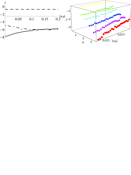
Figure 1: Left: Performance of CDD (solid line, $n=4$) vs PDD (dot-dashed line) as a function of random jitter fraction $|w_{P}|:=\left\|W_{P}\right\|/\left\|H_{P}\right\|$, with pulse-width $\delta=10^{-5}T$, coupling strength $j=.2/T$ ($T$ is the total evolution time), and number of bath spins $K=2$, averaged over $90$ jitter realizations. For comparison, the horizontal dashed line corresponds to free evolution. Right: CDD as a function of random jitter fraction $|w_{P}|$ and concatenation level $n$. The vertical axis denotes $l=\log_{10}(1-\text{purity})$ here and in Figs. 2 and 3.

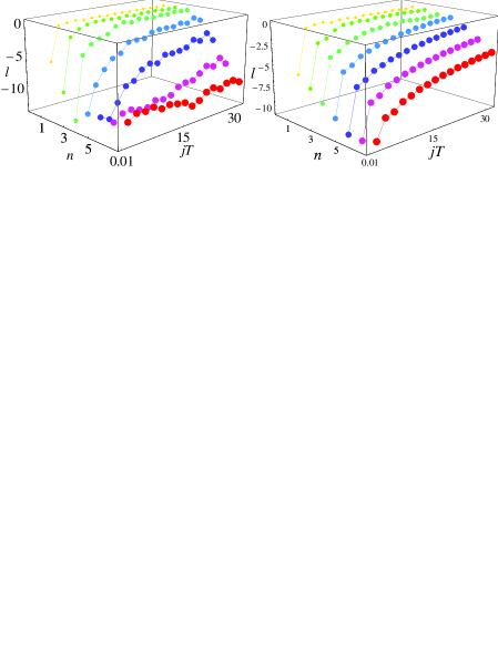
Figure 2: CDD (left) and PDD (right), as a function of system-bath coupling $j$; pulse width $\delta=10^{-4}T$, number of bath spins $K=5$, and without jitter ($W_{P}=0$). Note the $l$-axis scale difference between CDD and PDD.

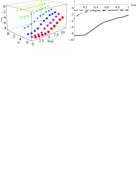
Figure 3: Left: CDD performance as a function of concatenation level and systematic jitter. The pulse width $\delta=10^{-4}T$, number of bath spins $K=5$, $jT=15.0$, averaged over $7-80$ realizations (more realizations for higher $n$). Right: CDD (solid line) vs PDD (dot-dashed line) as a function of systematic jitter for $n=5$, $\delta=10^{-5}T$ , $K=5$, $j\tau_{0}=3.0$, averaged over $14-80$ realizations. The dashed line is pulse-free evolution. CDD performance is unaffected up to $\sim 20\%$ jitter level.

Our simulation results, shown in Figs. 1-3, compare CDD and PDD as a function of coupling strength, relative jitter magnitude, and number of pulses. Fig. 1, left, compares CDD and PDD at fixed number of pulses. CDD outperforms PDD in the random jitter case with noise levels of up to almost $10\%$. Fig. 1, right, shows the performance of CDD as a function of jitter magnitude and concatenation level: the improvement is systematic as a function of the number of pulses used. Figure 2 contrasts CDD and PDD in the jitter-free case, as a function of system-bath coupling $j$. As predicted in the analytical treatment below, CDD offers improvement compared to PDD in decoherence reduction over a wide range of $j$ values. Figure 3 compares CDD and PDD as a function of systematic jitter. Superior performance of CDD is particularly apparent. These results establish the advantage of CDD over PDD in a model of significant practical interest, subject to a wide range of experimentally relevant errors. We now proceed to an analytical treatment.

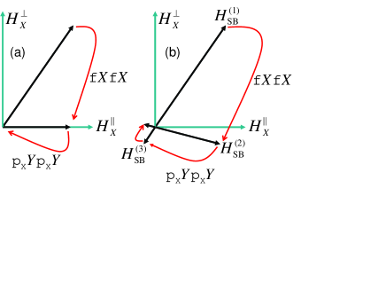
Figure 4: Projections involved in DD. (a) Perfect cancelation in first-order Magnus case. (b) Extra rotation induced by higher-order Magnus terms, and effect of concatenation.

Imperfect decoupling.— Consider DD pulse sequences composed of ideal pulses. Let us partition $H_{e}$ as $H_{e}=H_{X}^{\bot}+H_{X}^{\|}$, where $H_{X}^{\bot}=Y\otimes B_{y}+Z\otimes B_{z}$ and $H_{X}^{\|}=X\otimes B_{x}+H_{B}$. The super/subscripts $\bot,X$ and $\|,X$ correspond to terms that anti-commute and commute with $X\otimes I_{B}$, respectively. Thus the effect of p${}_{X}=$$\mathtt{f}X\mathtt{f}X$ in PDD can be viewed as a projection of $H_{SB}$ onto the component “parallel” to $X$, i.e., $H_{X}^{\|}$. For the $Y$ pulses in p${}_{1}=$p${}_{X}Y$p${}_{X}Y$ we can similarly write $H_{X}^{\|}=H_{Y}^{\bot}+H_{Y}^{\|}$, where $\bot,Y$ ($\|,Y$) denotes anti-commutation (commutation) with $Y$, whence $H_{Y}^{\|}=H_{B}$. Then the role of the $Y$ pulses is to project $H_{X}^{\|}$ onto $H_{Y}^{\|}$, which eliminates $H_{SB}$ altogether, i.e., transforms $H_{e}=H_{SB}+H_{B}$ into a “pure-bath” operator $H_{B}$. This geometrical picture of two successive projections is illustrated in Fig. 4(a). However, these projections are imperfect in practice due to second-order Magnus errors. Indeed, instead of a sequence such as $\mathtt{f}$$X$$\mathtt{f}$$X$, one has, after pulse $P_{i=X,Y}$, $I_{E,i}:=\exp[-i\tau(H_{i}^{\|}-H_{i}^{\bot})]\exp[-i\tau(H_{i}^{\|}+H_{i}^{\bot})]$, where $H_{e}=H_{i}^{\|}+H_{i}^{\bot}$, and we have accounted for the sign-flipping due to $P_{i}$. Using the BCH formula (e.g., Klarsfeld:89 ), we approximate the total unitary evolution as $I_{E,i}=\exp[-i(2\tau)H_{\mathrm{eff},i}+O\left(\lambda_{i}^{3}\right)]$, where $H_{\mathrm{eff},i}\!\!:=\!\!\mathcal{D}_{P_{i}}(\tau)[H_{e}]=e^{-i\tau H_{i}^{\bot}/2}H_{i}^{\|}e^{i\tau H_{i}^{\bot}/2}$, where $\lambda_{i}^{3}:=\tau^{3}\|H_{i}^{\bot}\|^{2}\|H_{i}^{\|}\|$, and it is assumed that, since $\|H_{e}\|<\infty$, one can pick $\tau$ such that $\lambda_{i}\ll 1$. The mapping $\mathcal{D}_{P_{i}}(\tau)[H_{e}]$ clearly has a geometric interpretation as a projection that eliminates $H_{i}^{\bot}$, followed by a rotation generated by $H_{i}^{\bot}$. This rotation produces extra system-bath terms besides $H_{i}^{\|}$, hence imperfect DD. This is illustrated in Fig. 4(b): in the first-order Magnus approximation the transition from $H_{\mathrm{SB}}^{(2)}$ to $H_{\mathrm{SB}}^{(3)}$ suffices to eliminate $H_{\mathrm{SB}}$, i.e., $H_{\mathrm{SB}}^{(3)}=0$. But in the presence of second-order Magnus errors $H_{\mathrm{SB}}^{(3)}\neq 0$. The difference between CDD and PDD is precisely in the manner in which this error is handled: in PDD the $H_{\mathrm{SB}}^{(3)}$ error accumulates over time since the same procedure is simply repeated periodically. However, in CDD the process of projection+rotation is continued at every level of concatenation, as suggested in Fig. 4(b) (red arrow above $H_{\mathrm{SB}}^{(3)}$). In CDD, $H_{\mathrm{SB}}^{(m)}$ is shrunk with increasing $m$, in a manner we next quantify.

Convergence of CDD in the limit of zero-width pulses.— Decoupling induces a mapping on the components of $H_{e}$. For a single qubit, writing $H_{e}=\sum_{\alpha=x,y,z}\sigma_{\alpha}\otimes B_{\alpha}$, we have $H_{e}\overset{\mathtt{p}_{1}}{\mapsto}H_{e}^{(1)}=\sum_{\alpha}\sigma_{\alpha}\otimes B_{\alpha}^{(1)}$, where a second-order Magnus expansion yields: $B_{0}^{(1)}=B_{0}$, $B_{x}^{(1)}=i\tau_{0}[B_{0},B_{x}]$, $B_{y}^{(1)}=i\tau_{0}\frac{1}{2}([B_{0},B_{y}]-i\{B_{x},B_{z}\})$, $B_{z}^{(1)}=0$. Let us define $\beta:=\left\|B_{0}\right\|$ and $J:=\max(\left\|B_{X}\right\|,\left\|B_{Y}\right\|,\left\|B_{Z}\right\|)$, where we assume $J<\beta<\infty$ foot2 . Comparing with the model we have used numerically, $J=O(\lambda)$ and $\beta=O(\omega_{B})$. It is possible to show that a concatenated pulse sequence $\mathtt{p}_{n}$ can still be consistently described by a second-order Magnus expansion at all levels of concatenation, provided the (sufficient) condition $\tau_{n}\beta\ll 1$ is satisfied supp-mat . We can then derive the recursive mapping relations for $H_{e}^{(n-1)}\overset{\mathtt{p}_{n}}{\mapsto}H_{e}^{(n)}=\sum_{\alpha}\sigma_{\alpha}\otimes B_{\alpha}^{(n)}$: $B_{0}^{(n\geq 0)}=B_{0}$, $B_{x}^{(n\geq\text{$1$})}=(i\tau_{n-1})[B_{0},B_{x}^{(n-1)}]$, $B_{y}^{(n\geq\text{$2$})}=\frac{1}{2}(i\tau_{n-1})[B_{0},B_{y}^{(n-1)}]$, $B_{z}^{(n\geq\text{$1$})}=0$. The propagator corresponding to the whole sequence is $\exp(-i\tau_{n}H_{e}^{(n)})$, which in the limit of ideal performance reduces to the identity operator. These results for $B_{\alpha}^{(n)}$ allow us to study the convergence of CDD, and bound the success of the DD procedure, as measured in terms of the fidelity (state overlap between the ideal and the decoupled evolution). This fidelity is given by Terhal:04

$$f_{n}\approx 1-||\tau_{n}\widetilde{H}_{e}^{(n)}||^{2}\approx 1-(\tau_{n}h^{(n)})^{2}=:1-(\Phi_{\text{CDD}})^{2},$$ (1)

where $\widetilde{H}$ is the system-traceless part of $H$, and $h^{(n)}:=\max\{||B_{x}^{(n)}||,||B_{y}^{(n)}||\}$. We find that

$$\Phi_{\text{CDD}}\leq(\beta T/N^{1/2})^{n}(JT),$$ (2)

where $T=N\tau_{0}\lesssim\tau_{n}=4^{n}\tau_{0}$ is the total sequence duration, comprised of $N$ pulse intervals. In contrast, $\Phi_{\text{PDD}}=Th^{(1)}$ yields

$$\Phi_{\text{PDD}}=2(\beta\tau_{0})(JT)=2(\beta T/N)(JT).$$ (3)

Note that for $N=4$, $\Phi_{\text{CDD}}=\Phi_{\text{PDD}}$ as expected. There is a physical upper limit to the number of concatenation levels, imposed by the condition $\beta\tau_{n}\ll 1$. Using this condition in the form $\beta=c/T$, where $c$ is some small constant (such as $0.1$), and fixing the value of $\beta$, we can back out an upper concatenation level $n_{\max}=-\log_{4}\frac{\beta\tau_{0}}{c}$; inserting this into Eq. (2) we have $\Phi_{\text{CDD}}\leq(c\beta\tau_{0})^{-\frac{1}{2}\log_{4}\frac{\beta\tau_{0}}{c}}(JT)$. We can now compare the CDD and PDD bounds in term of the final fidelity:

$$\frac{1-f_{\text{CDD}}}{1-f_{\text{PDD}}}\leq\frac{(c\beta\tau_{0})^{-\log_{4}\frac{\beta\tau_{0}}{c}}}{4(\beta\tau_{0})^{2}}\overset{\beta\tau_{0}\rightarrow 0}{\longrightarrow}0.$$ (4)

This key result shows that CDD converges super-polynomially faster to zero in terms of the (physically relevant) parameter $\beta\tau_{0}$, at fixed pulse sequence duration. However, it is important to emphasize that our bound on $\Phi_{\text{CDD}}$ is unlikely to be very tight, since we have been very conservative in our estimates (e.g., in applying norm inequalities and estimating convergence domains). Indeed, in our simulations (above) $\beta\tau_{n}\approx 2$, which is beyond our conservatively obtained convergence domain.

Finite width pulses.— We now briefly consider the more realistic scenario of rectangular pulses $\mathcal{T}\exp[-i\int_{0}^{\delta}\{H_{P}(t)+H_{e}(t)\}dt]$ of width $\delta\ll\tau_{0}$. In this case we can derive a modified form of the condition $\beta\tau_{n}\ll 1$, required for consistency (of using a second-order Magnus expansion at all levels of concatenation) supp-mat :

$$c\tau_{n}\beta+d\frac{\delta}{\tau_{n}}\ll 1,$$ (5)

where $c,d\sim 1$ are pulse sequence-specific numerical factors. The consistency requirement (5) validates the analysis of convergence of CDD for $\delta\neq 0$, and we can reproduce the advantage of CDD over PDD for $\delta=0$ [manifest in Eq. (4)]. As expected Eq. (5) imposes a more demanding condition on the total duration $\tau_{n}$, at fixed bath strength $\beta$. While Eq. (5) cannot be called a threshold condition (in analogy to the threshold in QEC), since it depends on the total sequence duration, it does provide a useful sufficient condition for convergence of a finite pulse-width CDD sequence, and introduces the concept of error per gate which is fundamental in QEC.

Conclusions and outlook.— We have shown that concatenated DD pulses offer superior performance to standard, periodic DD, over a range of experimentally relevant parameters, such as system-bath coupling strength, and random as well as systematic control errors. Here we have addressed the preservation of arbitrary quantum states. Quantum computation can in principle be performed, using CDD, over encoded qubits by choosing the DD pulses as the generators of a stabilizer QECC, and the quantum logic operations as the corresponding normalizer ByrdLidar:01a ; ByrdLidar:03 . Another intriguing possibility is to combine CDD and high-order composite pulse methods Brown:04 .

- (1) R. Freeman, Spin Choreography: Basic Steps in High Resolution NMR (Oxford University Press, Oxford, 1998).
- (2) L. Viola, E. Knill and S. Lloyd, Phys. Rev. Lett. 82, 2417 (1999).
- (3) P. Zanardi, Phys. Lett. A 258, 77 (1999).
- (4) E. Knill, R. Laflamme, and L. Viola, Phys. Rev. Lett. 84, 252 (2000).
- (5) A.M. Steane, Phys. Rev. A 68, 042322 (2003).
- (6) B.M. Terhal and G. Burkard, Phys. Rev. A 71, 012336 (2005).
- (7) P. Facchi et al., Phys. Rev. A 71, 022302 (2005).
- (8) L. Viola and E. Knill, Phys. Rev. Lett. 90, 037901 (2003).
- (9) H. Rabitz et al., Science 288, 284 (2000).
- (10) We use the spectral radius ; a convenient unitarily-invariant operator norm, which, for normal operators, coincides with the largest absolute eigenvalue.
- (11) This has been observed also in QECC work dealing with general error models Knill:99a ; Terhal:04 , but as has been pointed out there, if it must be appropriately redefined.
- (12) L. Viola, J. Mod. Optics 51, 2357 (2004).
- (13) U. Haeberlen and J. S. Waugh, Phys. Rev. 175, 453 (1968); H.M. Cho, R. Tycko, and A. Pines, Phys. Rev. Lett. 56, 1905 (1986).
- (14) N.V. Prokof’ev and P.C.E. Stamp, Rep. Prog. Phys. 63, 669 (2000).
- (15) R. de Sousa, S. Das Sarma, Phys. Rev. B 68, 115322 (2003).
- (16) G. Burkard, D. Loss and D.P. DiVincenzo, Phys. Rev. B 59, 2070 (1999).
- (17) B.E. Kane, Nature 393, 133 (1998).
- (18) S. Klarsfeld, J.A. Oteo, J. Phys. A 22, 4565 (1989).
- (19) This assumption is made to simplify some of our convergence arguments; while it is not essential, it is reasonable, since we expect only a small number of bath degrees of freedom to be coupled to a given qubit, whereas no restriction exists on the bath self-Hamiltonian
- (20) K. Khodjasteh and D.A. Lidar, in preparation.
- (21) M.S. Byrd and D.A. Lidar, Phys. Rev. Lett. 89, 047901 (2002).
- (22) M.S. Byrd and D.A. Lidar, J. Mod. Optics 50, 1285 (2003).
- (23) K.R. Brown, A.W. Harrow, I.L. Chuang, Phys. Rev. A 70, 052318 (2004).