Kraus representation of damped harmonic oscillator and its application

Abstract

By definition, the Kraus representation of a harmonic oscillator suffering from the environment effect, modeled as the amplitude damping or the phase damping, is directly given by a simple operator algebra solution. As examples and applications, we first give a Kraus representation of a single qubit whose computational basis states are defined as bosonic vacuum and single particle number states. We further discuss the environment effect on qubits whose computational basis states are defined as the bosonic odd and even coherent states. The environment effects on entangled qubits defined by two different kinds of computational basis are compared with the use of fidelity.

I introduction

Since the fast quantum algorithms were developed, the quantum information and computation have aroused great enthusiasm among physicists because of their potential applications. The basic unit of the classical information is a bit, which can only have a choice between two possible classical states denoted by $0$ or $1$. The information carriers in the quantum communication and computation are called quantum bits or qubits. The main difference between the qubit and the classical bit is that the qubit is defined as a quantum superposition of two orthogonal quantum states usually written as $|0\rangle$ and $|1\rangle$ called as the computational basis states. It means that the qubit has an infinite number of choices of the states $\alpha|0\rangle+\beta|1\rangle$ with the condition $|\alpha|^{2}+|\beta|^{2}=1$. It is obvious that the superposition principle allows application of quantum states to simultaneously represent many different numbers, this is called the quantum parallelism, which enables the quantum computation to solve some problems, such as factorization, intractable on a classical computer.

However, a pure quantum superposition state is very fragile. A quantum system cannot be isolated from the environment, it is always open and interacts with the uncontrollable environment. This unwanted interaction induces entanglement between the quantum system and the environment such that the pure superposition state is destroyed, which results in an inevitable noise in the quantum computation and information processing. Unlike a closed system, whose final state $\rho^{\prime}$ can be obtained by a unitary transformation $U$ of the initial state $\rho$ as $\rho^{\prime}=U\rho U^{\dagger}$, the final state of an open system cannot be described by a unitary transformation of the initial state. Quantum operation formalism is usually used to describe the behavior of an open quantum system in which the final state $\rho^{\prime}$ and the initial state $\rho$ can be related by a quantum operation ${\cal E}$ as $\rho^{\prime}={\cal E}(\rho)$. In general, the quantum operation ${\cal E}$ on the state $\rho$ can be described by the Kraus operator-sum formalism Kraus ; MI as ${\cal E}(\rho)=\sum_{\mu}E_{\mu}\rho E^{\dagger}_{\mu}$ where the operation elements $E_{\mu}(E^{\dagger}_{\mu})$ satisfy the completeness relation $\sum_{\mu}E^{\dagger}_{\mu}E_{\mu}=I$. Operators $E_{\mu}$ act on the Hilbert space $H_{S}$ of the system. They can be expressed as $E_{\mu}=\langle e_{\mu}|U_{t}|e_{0}\rangle$ by the total unitary operator $U_{t}$ of the system and the environment with an orthonormal basis $|e_{\mu}\rangle$ for the Hilbert space $H_{E}$ and the initial state $\rho_{E}=|e_{0}\rangle\langle e_{0}|$ of the environment. This elegant representation is extensively applied to describe the quantum information processing  B ; N .

In practice, the environment effect on the quantum system is a more complicated problem. There are two ideal models of noise called the amplitude and phase damping, which can capture many important features of the noise MI . They are applied in many concrete discussions to model noise of the quantum information processing, e.g., reference lidar . As a system, a single-mode harmonic oscillator is the simplest and most ideal model to represent a single mode light field, vibration phonon mode, or excitonic wave. For convenience, we refer this harmonic oscillator to a single-mode light field in this paper. A study of a single harmonic oscillator suffering from damping is expected to give us an easier grasp of the nature of damping. The Kraus representation of a harmonic oscillator suffering from the above two kinds of noise has been given by Chuang et al., simply modeling environment as a single mode oscillator MI ; isaac . However generally speaking, the environment is usually described as a system of multimode oscillators for both the phase damping and amplitude damping. Milburn et al. have also given the Kraus representation of a harmonic oscillator suffering from the amplitude damping by modeling the environment as a system of the multimode oscillators using the quantum measurement theory milburn . Although there are many studies about Kraus representation, e.g. in Refs. Kraus ; lidar ; kraus2 , to the best of our knowledge, there is no proof of the Kraus representation for a harmonic oscillator suffering from amplitude damping or phase damping by directly using its definition when the environment is modeled as a system of multimode oscillators. In view of the importance of the Kraus representation in the quantum information, we would like to revisit this question in this paper. We will extend the proof of Chuang et al., that is, we will give the Kraus representation using a simple operator algebra method by modeling the system as a single mode oscillator and the environment as multimode oscillators according to the definition of the Kraus representation.

Our paper is organized as follows. In Sec. II, we give the Kraus representation for the amplitude damping case, then we discuss the effect of the environment on a qubit whose computational basis is defined by odd and even coherent states with decay of at most one particle, we compare this result with that of a qubit defined by vacuum and single photon number states. In Sec. III, we give the Kraus representation for the phase damping case, and explain its effect. Similar to the analysis in Sec. II, we also compare the effect of the phase damping on the entangled qubit defined by different states. Finally, we give our conclusions in Sec. IV.

II amplitude damping

II.1 Kraus representation

One of the most important reasons for the quantum state change is the energy dissipation of the system induced by the environment. This energy dissipation can be characterized by an amplitude damping model. Ideally we can model the system, for example, a single mode cavity field, as a harmonic oscillator, which is coupled to the environment modeled as multimode oscillators. Then the whole Hamiltonian of the system and the environment can be written as

$$H=\hbar\omega b^{\dagger}b+\hbar\sum_{i}\omega_{i}b_{i}^{\dagger}b_{i}+\hbar\sum_{i}g_{i}(b^{\dagger}b_{i}+bb^{\dagger}_{i})$$ (1)

under the rotating wave approximation, where $b(b^{\dagger})$ is the annihilation (creation) operator of the harmonic oscillator of frequency $\omega$, and $b_{i}(b^{\dagger}_{i})$ is the annihilation (creation) operator of the $i$th mode of the environment with frequency $\omega_{i}$, $g_{i}$ is coupling constant between the system and the $i$th mode of the environment. We assume that the initial state of the whole system is

$$\rho(0)=\rho_{S}(0)\otimes\rho_{E}(0),$$ (2)

where $\rho_{S}(0)$ and $\rho_{E}(0)$ denote the initial states of the system and environment respectively. With the time evolution, the initial state evolves into

$$\rho(t)=U(t)\rho_{S}(0)\otimes\rho_{E}(0)U^{\dagger}(t)$$ (3)

with $U=\exp(-iHt/\hbar)$. Since we are only interested in the time evolution of the system, we perform a partial trace over the environment and find the reduced density operator of the system as

$$\rho_{S}(t)={\rm Tr}_{E}\left\{U(t)\rho_{S}(0)\otimes\rho_{E}(0)U^{\dagger}(t)\right\}$$ (4)

$$=\sum_{\{k_{i}\}}\langle\{k_{i}\}|U(t)\rho_{S}(0)\otimes\rho_{E}(0)U^{\dagger}(t)|\{k_{i}\}\rangle$$

where $\{|\{k_{i}\}\rangle\equiv|k_{1}\cdots k_{i}\cdots\rangle=\Pi_{i}\otimes|k_{i}\rangle\}$ is an orthonormal basis of the Hilbert space $H_{E}$ for the environment, and $k_{i}$ denotes that there are $k_{i}$ bosonic particles in the $i$th mode. We assume that the environment is at zero temperature, so its initial state is in the vacuum state $|\{0\}\rangle\equiv\Pi_{i}\otimes|0_{i}\rangle=|\cdots 0\cdots\rangle$ of multimode harmonic oscillators. The Hilbert space $H_{E}$ can be decomposed into a direct sum of many orthogonal subspaces $H_{k}$ as $H_{E}=\bigoplus_{k=0}^{\infty}H_{k}$ with an orthonormal basis $\{|\{k_{i}\}\rangle\}$, which satisfies the condition $\sum_{i=1}^{\infty}k_{i}=k$ for each subspace $H_{k}$. So we can regroup the summation in Eq.(4) and define the quantum operation element $A_{k}$ as follows

$$A_{k}(t)=\sum_{\{k_{i}\}}^{k}{{}^{\prime}}\ \langle\{k_{i}\}|U(t)|\{0\}\rangle$$ (5)

which acts on the Hilbert space $H_{S}$ of the system. Hereafter, $\sum{{}^{\prime}}$ stands for summation under the condition $\sum_{i}k_{i}=k$; $A_{k}(t)$ means that there are $k$ bosonic particles absorbed by the environment through the evolution over a finite time $t$, and $A^{\dagger}_{k}(t)$ denotes the Hermitian conjugate of $A_{k}(t)$. Then Eq.(4) can be rewritten by virtue of the operation elements $A_{k}(t)$ and its Hermitian conjugate $A^{\dagger}_{k}(t)$ as a concise form called the Kraus representation MI

$$\rho_{S}(t)=\sum_{k=0}^{\infty}A_{k}(t)\rho_{S}(0)A^{\dagger}_{k}(t).$$ (6)

It is very easy to check that the elements $A_{k}(t)$ satisfy the relation $\sum_{k}A^{\dagger}_{k}(t)A_{k}(t)=I$. In order to further give the solution of the operator $A_{k}(t)$, we first use the number state $|n\rangle$ of the system to define an orthonormal basis $\{|n\rangle\}$ of the Hilbert space $H_{S}$ of the system. Then the matrix representation of the operator $A_{k}(t)$ can be written as

$$A_{k}(t)=\sum_{m,n}A_{m,n}^{k}(t)|m\rangle\langle n|$$ (7)

with the matrix element

$$A_{m,n}^{k}(t)=\sum_{\{k_{i}\}}^{k}{{}^{\prime}}\ \langle m|\langle\{k_{i}\}|U(t)|\{0\}\rangle|n\rangle.$$ (8)

Because the state $U(t)|\{0\}\rangle|n\rangle$ can be written as $U(t)(b^{\dagger})^{n}/\sqrt{n!}|\{0\}\rangle|0\rangle=[b^{\dagger}(-t)]^{n}/\sqrt{n!}|\{0\}\rangle|0\rangle$. Using the Wigner-Weisskopf approximation ll , the operator $b^{\dagger}(t)$ can be obtained by solving the Heisenberg operator equation of motion for Hamiltonian (1) as

$$b^{\dagger}(t)=u(t)b^{\dagger}(0)+\sum_{i=1}^{\infty}v_{i}(t)b^{\dagger}_{i}(0),$$ (9)

where $u(t)=\exp{(-\frac{\gamma}{2}t+i\omega t)}$ and the Lamb shift has been neglected. The damping rate $\gamma$ is defined as $\gamma=2\pi\epsilon(\omega)|g(\omega)|^{2}$ with a spectrum density $\epsilon(\omega)$ of the environment. The details of the time dependent parameter $v_{i}(t)$ can be found in  ll ; sun . We can use Eq.(9) to expand $U(t)|\{0\}\rangle|n\rangle$ as many terms characterized by the particle number $k$ lost from the system, and each term with fixed $k$ can be expressed as

$$\left[u^{*}(t)\right]^{n-k} \sqrt{\frac{1}{k!}\left(\begin{array}[]{c}n\\ k\end{array}\right)}\sum_{i_{1}\cdots\neq i_{q}\cdots\neq i_{k}=0}^{\infty}\sum_{\{l_{i}\}}^{k}{{}^{\prime}}\,\frac{k!}{l_{1}!\cdots l_{k}!}$$ (13)

$$\times\prod_{q=1}^{k}\left(v^{*}_{i_{q}}(t)b^{\dagger}_{i_{q}}(0)\right)^{l_{q}}|\{0\}\rangle|n-k\rangle.$$

By using Eqs.(7)-(13), we can obtain the product of the matrix elements of $A^{k}_{m,n}$ and its Hermitian conjugate as

$$A^{k}_{m,n}({A^{k}}_{m,n})^{\dagger}=\left(\begin{array}[]{c}n\\ k\end{array}\right)[\eta(t)]^{(n-k)}[1-\eta(t)]^{k}\delta_{m,n-k}$$ (14)

with $\eta(t)=e^{-\gamma t}$, where we have used the completeness of the subspace with fixed $k$

$$\sum_{\{k_{i}\}}^{k}{{}^{\prime}}\ |\{k_{i}\}\rangle\langle\{k_{i}\}|=1,$$ (15)

and condition $|u(t)|^{2}+\sum_{i}|v_{i}(t)|^{2}=1$, which comes from the commutation relation $\left[b(t),b^{\dagger}(t)\right]=1$. It is clear that the non-zero matrix element $A^{k}_{m,n}(t)$ must satisfy the relation $n-m=k$, and all contributions to the elements of the quantum operation $A_{k}(t)$ come from the states $|n\rangle$ satisfying the condition $n\geq k$. Then we can take each matrix element $A^{k}_{m,n}(t)$ as a real number and finally obtain isaac ; milburn

$$A_{k}(t)=\sum_{n=k}^{\infty}\sqrt{\left(\begin{array}[]{c}n\\ k\end{array}\right)}[\eta(t)]^{(n-k)/2}[1-\eta(t)]^{k/2}|n-k\rangle\langle n|.$$ (16)

It is not difficult to prove that $\sum_{k}A^{\dagger}_{k}(t)A_{k}(t)=1$. In Eq.(16), one finds that$(1-\eta(t))^{k/2}$ is the probability that the system loses $k$ particles up to time $t$, or the probability that the state $|n\rangle$ is undecayed corresponds to $[\eta(t)]^{(n-k)/2}$ for $k$ particle decay process up to time $t$. For the convenience, we will write $\eta(t)$ as $\eta$ in the following expressions.

Using a single qubit $\rho$ defined by the bosonic number state $\{|0\rangle,\hskip 0.28453pt|1\rangle\}$ as the computational basis states, we can simply demonstrate how to give its Kraus representation when it suffers from the amplitude damping. By Eq.(16), it is very easy to find that the quantum operation on qubit $\rho$ includes only two operational elements $A_{0}$ and $A_{1}$, that is

$${\cal E}(\rho)=A_{0}\rho A^{\dagger}_{0}+A_{1}\rho A^{\dagger}_{1}$$ (17)

with

$$A_{0}(t) = |0\rangle\langle 0|+\sqrt{\eta}|1\rangle\langle 1|,$$ (18a)

$$A_{1}(t) = \sqrt{1-\eta}|0\rangle\langle 1|,$$ (18b)

where $\sqrt{1-\eta}$ is the probability that the system lose one particle up to time $t$.

II.2 Effect of amplitude damping on qubits

In this subsection, we will demonstrate an application of the above conclusions about the Kraus representation. We know that two kinds of logical qubits, whose computational basis states are defined by using the bosonic even and odd coherent states haroche or vacuum and bosonic single particle number states, are accessible in experiments. For brevity, we refer to qubits defined via the even and odd coherent states as the (Schrödinger) cat-state qubits by contrast to the Fock-state qubits defined by vacuum and single-photon states in the following expressions. It has been shown that the bit flip errors caused by a single decay event, which results from the spontaneous emissions, are more easily corrected by a standard error correction circuit for the logical qubit defined by the bosonic even and odd coherent states ptc than that defined by the bosonic vacuum and single particle number states. We know that the entangled qubit takes an important role in the quantum information processing. So in the following, we will study the effect of the environment on entangled qubits defined by the above two kinds of computational basis states when they are subject to at most one decay event caused by the amplitude damping. Let $|\alpha\rangle$ be a bosonic coherent state (we denote this single bosonic mode as a single-mode light field, but it can be generalized to any bosonic mode, for example, excitonic mode, vibrational mode of trap ions and so on). In general, if a single-mode light field, which is initially in the coherent state $|\alpha\rangle$, suffers from amplitude damping, the Kraus operation element (16) changes it as follows

$$A_{k}|\alpha\rangle=e^{-\frac{(1-\eta)|\alpha|^{2}}{2}}\frac{(\alpha\sqrt{1-\eta})^{k}}{\sqrt{k!}}|\sqrt{\eta}\alpha\rangle,$$ (19)

and the normalized state, which is denoted by ${\cal N}[A_{k}|\alpha\rangle]$, can be written as

$${\cal N}[A_{k}|\alpha\rangle]=|\sqrt{\eta}\alpha\rangle,$$ (20)

which means that the coherent state remains coherent under the amplitude damping, but its amplitude $\alpha$ is reduced to $\sqrt{\eta}\alpha$ due to the interaction with the environment.

Now we define a logical zero-qubit state $|0\rangle_{L}$ and a logical one-qubit state $|1\rangle_{L}$ using the even and odd coherent states as

$$|0\rangle_{L} = N_{+}(|\alpha\rangle+|-\alpha\rangle)$$

$$|1\rangle_{L} = N_{-}(|\alpha\rangle-|-\alpha\rangle)$$ (21)

with $N_{\pm}=(2\pm 2e^{-2|\alpha|^{2}})^{-\frac{1}{2}}$ and subscript $L$ denotes the logical state. If we know that the system loses at most one photon with the time evolution but we do not have the detailed information on the lost photons. Then, we only need to calculate two Kraus operators $A_{0}$ and $A_{1}$ corresponding to no-photon and single-photon decay events, respectively.

No-photon decay event changes the logical qubits $|0\rangle_{L}$ and $|1\rangle_{L}$ as follows

$$|\widetilde{0}\rangle = {\cal N}[A_{0}|0\rangle_{L}]=N^{\prime}_{+}\left(|\sqrt{\eta}\alpha\rangle+|-\sqrt{\eta}\alpha\rangle\right),$$ (22)

$$|\widetilde{1}\rangle = {\cal N}[A_{0}|1\rangle_{L}]=N^{\prime}_{-}\left(|\sqrt{\eta}\alpha\rangle-|-\sqrt{\eta}\alpha\rangle\right),$$ (23)

where $|\widetilde{0}\rangle$ and $|\widetilde{1}\rangle$ are normalized states of $A_{0}|0\rangle_{L}$ and $A_{0}|1\rangle_{L}$ with the normalized constants $N^{\prime}_{\pm}=\left\{2\pm 2\exp(-2\eta|\alpha|^{2})\right\}^{-1/2}$. It is obvious that no-photon decay event reduces only the intensity of the logical qubit, leaving the even and odd properties of the logical qubit states unchanged. A simple analysis of how the noisy channel affects the original quantum state can be made by calculating the fidelity defined as the average value of the final reduced density matrix $\rho(t)$ with initial pure state $|\psi\rangle$, that is $f(t)=\langle\psi|\rho|\psi\rangle$. The fidelity $f_{i}(t)$ of the qubit state (21) with no-photon decay event can be obtained as

$$f_{i}(t)=\frac{(e^{\sqrt{\eta}|\alpha|^{2}}+(-1)^{i}e^{-\sqrt{\eta}|\alpha|^{2}})^{2}}{(e^{|\alpha|^{2}}+(-1)^{i}e^{-|\alpha|^{2}})(e^{\eta|\alpha|^{2}}+(-1)^{i}e^{-\eta|\alpha|^{2}})}$$ (24)

with $i=0,\ 1$, which denotes zero-qubit state or one-qubit state. But for a single-photon decay event, we can have the following

$$|\widetilde{1}\rangle={\cal N}[A_{1}|0\rangle_{L}],\hskip 28.45274pt|\widetilde{0}\rangle={\cal N}[A_{1}|1\rangle_{L}].$$ (25)

We find that the single photon decay event flips an even coherent state to an odd coherent state with the reduction of the amplitude and vice versa. It is very easy to prove that

$$|\widetilde{1}\rangle = {\cal N}[A_{(2m+1)}|0\rangle_{L}]={\cal N}[A_{2m}|1\rangle_{L}],$$ (26)

$$|\widetilde{0}\rangle = {\cal N}[A_{(2m+1)}|1\rangle_{L}]={\cal N}[A_{2m}|0\rangle_{L}]$$ (27)

with $m=0,\ 1,\ 2\cdots$, which means that the even number of photons decay event only reduces the intensity of the logical signal, and keeps the even and odd properties of the logical state unchanged; but the odd number of photons decay event flips a qubit causing error and reduces the intensity of the qubit signal. If the coherent amplitude of the cat states is infinitely large, that is, $|\alpha|\rightarrow\infty$, then we find that the fidelity $f_{i}(t)\approx 1$ with a larger $\eta$, so under this condition, we can say that the no-photon decay event essentially leaves the logical qubit states unchanged and the single-photon decay event causes a qubit flip error. It means that the use of the even and odd coherent states as logical qubit states $|0\rangle_{L}$ and $|1\rangle_{L}$ is better than the use of the vacuum state $|0\rangle$ and single-photon state $|1\rangle$ as logical qubit states in the amplitude damping channel with a few photons loss. Because the single-photon decay event changes vacuum and single-photon states to $A_{1}|0\rangle=0$ and $A_{1}|1\rangle=|0\rangle$, the single-photon decay event is an irreversible process for vacuum and single-photon states.

An entangled pair of qubits, whose computational basis states are defined by the even and odd coherent states (21), can be written as

$$|\Psi\rangle=\frac{1}{\sqrt{2}}\left\{|0\rangle_{L}|1\rangle_{L}+|1\rangle_{L}|0\rangle_{L}\right\}.$$ (28)

On the basis of the above discussions, we can study the effect of environments on entangled qubits when each mode loses at most one photon. For simplicity, two modes are assumed to suffer from effect of two same independent environments. There is no direct interaction between two systems. After the environment performs the following four measurements $\{E_{0}=A_{0}\otimes A_{0},\hskip 2.84544ptE_{1}=A_{0}\otimes A_{1},\hskip 2.84544ptE_{2}=A_{1}\otimes A_{0},\hskip 2.84544ptE_{3}=A_{1}\otimes A_{1}\}$ with $A_{0}$ an $A_{1}$ determined by Eq.(16), the entangled qubit (28) becomes the following mixed state

$$\rho(t) = \frac{\sum_{i=0}^{3}E_{i}\rho(0)E_{i}^{\dagger}}{{\rm Tr}\left\{\sum_{i=0}^{3}E_{i}\rho(0)E_{i}^{\dagger}\right\}}=\tilde{N}\left\{2p|\alpha|^{2}\left(\frac{N_{-}^{\prime 2}}{N_{+}^{\prime 2}}|\tilde{0}\tilde{0}\rangle\langle\tilde{0}\tilde{0}|\right.\right.$$ (29)

$$\left.+\frac{N_{+}^{\prime 2}}{N_{-}^{\prime 2}}|\tilde{1}\tilde{1}\rangle\langle\tilde{1}\tilde{1}|+|\tilde{0}\tilde{0}\rangle\langle\tilde{1}\tilde{1}|+|\tilde{1}\tilde{1}\rangle\langle\tilde{0}\tilde{0}|\right)$$

$$\left.+(1+p^{2}|\alpha|^{4})(|\tilde{0}\tilde{1}\rangle+|\tilde{1}\tilde{0}\rangle)(\langle\tilde{0}\tilde{1}|+\langle\tilde{1}\tilde{0}|)\right\}$$

with $p=1-\eta$ and the normalized constant

$$\widetilde{N}^{-1} = 2\frac{(1+p|\alpha|^{2})^{2}-e^{-4\eta|\alpha|^{2}}(1-p|\alpha|^{2})^{2}}{1-e^{-4\eta|\alpha|^{2}}}.$$ (30)

The fidelity $F_{1}(t)$ of the entangled qubit $|\Psi\rangle$ with at most one photon decay for each mode can be calculated as

$$F_{1}(t) = \langle\Psi|\rho(t)|\Psi\rangle$$

$$= \frac{\left(1+|\alpha|^{4}p^{2}\right){\rm csch}(2|\alpha|^{2}){{\rm sh}^{2}(2\sqrt{\eta}|\alpha|^{2})}}{2|\alpha|^{2}p\ {\rm ch}(2|\alpha|^{2}\eta)+\left(1+|\alpha|^{4}p^{2}\right){\rm sh}{(2|\alpha|^{2}\eta)}},$$

If each mode can dissipate any number of photons, but we know nothing about the details of dissipation, then we must sum up all possible environment measurements on the system, obtaining the reduced matrix operator of the system as

$$\rho^{\prime}(t)=\frac{1}{2-2e^{-4|\alpha|^{2}}}\left\{|\beta\rangle|\beta\rangle\langle\beta|\langle\beta|+|-\beta\rangle|-\beta\rangle\langle-\beta|\langle-\beta|\right\}$$

$$-\frac{M}{2-2e^{-4|\alpha|^{2}}}\left\{|-\beta\rangle|-\beta\rangle\langle\beta|\langle\beta|+|\beta\rangle|\beta\rangle\langle-\beta|\langle-\beta|\right\}$$ (32)

with $M=e^{-4|\alpha|^{2}(1-e^{-\gamma t})}$ and $|\beta\rangle=|u(t)\alpha\rangle$. Then we obtain the fidelity $F_{2}(t)$ as

$$F_{2}(t)={\rm ch}(2|\alpha|^{2}p)\,{{\rm csch}^{2}(2|\alpha|^{2})}\,{{\rm sh}^{2}(2\sqrt{\eta}|\alpha|^{2})}.$$ (33)

We can find that the logical state $|0\rangle_{L}$ and $|1\rangle_{L}$ in Eq.(28) can be reduced to the vacuum state $|0\rangle$ and single-photon state $|1\rangle$, respectively in the limit of the weak light field $|\alpha|\rightarrow 0$. It is easy to check that

$$A_{0}|0\rangle = |0\rangle,\hskip 14.22636ptA_{0}|1\rangle=\sqrt{\eta}|1\rangle,$$ (34)

$$A_{1}|0\rangle = 0,\hskip 22.76228ptA_{1}|1\rangle=\sqrt{1-\eta}|0\rangle$$ (35)

which means that the $|0\rangle$ qubit state is invariant when no-photon decay event happens, but the amplitude of the $|1\rangle$ qubit state is reduced to $\sqrt{\eta}$. If the system leaks one photon, then the $|0\rangle$ qubit state vanishes and the $|1\rangle$ qubit state returns to the $|0\rangle$ with the probability $\sqrt{1-\eta}$. The entangled qubit, whose computational basis states are defined by vacuum and single-photon states, can be written as

$$|\Psi\rangle=\frac{1}{\sqrt{2}}(|0\rangle|1\rangle+|1\rangle|0\rangle)$$ (36)

which can be obtained by setting $|\alpha|\rightarrow 0$ in Eq.(28). We can use the same step to obtain the fidelity $F^{\prime}_{1}(t)$ corresponding to Eq.(36) when both modes are subject to the amplitude damping as

$$F^{\prime}_{1}(t)=\eta(t),$$ (37)

where we assume that the damping is the same for the two modes. When the weak light field limit $|\alpha|\rightarrow 0$ is taken, we find that Eq.(II.2) and Eq.(33) can be written as

$$F_{1}(t) = \eta+\frac{\eta}{3}(1-5\eta+3\eta^{2}+\eta^{3})|\alpha|^{4}+{\cal O}(|\alpha|^{8}),$$

$$F_{2}(t) = \eta+\frac{2}{3}\eta(1-4\eta+3\eta^{2})|\alpha|^{4}+{\cal O}(|\alpha|^{8}).$$ (38)

It is clear that all the higher order terms of $|\alpha|^{2}$ can be neglected in the limit $|\alpha|\rightarrow 0$, so Eq.(II.2) and Eq.(33) can return to $F^{\prime}_{1}(t)$ in the weak field approximation.

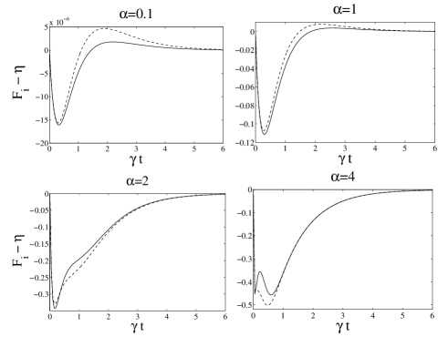
Figure 1: Difference of fidelities: $F_{1}-\eta$ (solid curves), given by Eqs. (II.2) and (37), and $F_{2}-\eta$ (dashed curves), given by Eqs. (33) and (37), versus scaled time $\gamma t$ for different values of amplitude $\alpha$.

By recalculating the difference

$$F_{1}(t)-F_{2}(t)=-\frac{1}{3}\eta(1-\eta)^{3}|\alpha|^{4}+{\cal O}(|\alpha|^{8}),$$ (39)

it is clear that fidelity $F_{1}(t)$ is less than $F_{2}(t)$ in the low-intensity regime. These predictions are confirmed by the exact evolution of fidelities depicted in Fig. (1) for $|\alpha|\leq 1$. To compare the fidelities in the short-time evolution, we expand the difference of Eqs. (II.2) and (33) in power series in $\Gamma t$ as follows

$$F_{1}(t)-F_{2}(t) = -\frac{2}{3}|\alpha|^{6}{\rm coth}(2|\alpha|^{2})(\gamma t)^{3}+{\cal O}\{(\gamma t)^{4}\}$$

which shows that $F_{1}(t)$ is less than $F_{2}(t)$ for arbitrary intensities in the short-time regime although the difference might be very small as presented in Fig. (1) for $|\alpha|=2,4$. In the long-time limit, we can expand the difference in a series of $\eta$ resulting in

$$F_{1}(t)-F_{2}(t) = \frac{2|\alpha|^{2}}{{\rm sh}(2|\alpha|^{2})}[1+|\alpha|^{4}-2|\alpha|^{2}{\rm coth}(2|\alpha|^{2})]\eta$$ (41)

$$+{\cal O}\{\eta^{2}\}$$

which is negative only for the intensity $|\alpha|^{2}<1.1997\cdots$. For higher intensity, we find that $|\widetilde{1}\rangle\approx|1\rangle_{L}$ and $|\widetilde{0}\rangle\approx|0\rangle_{L}$, and $p=1-\eta$ will become small with the time evolution, then the fidelity $F_{1}(t)$ will become greater than the fidelity $F_{2}(t)$ in some regimes. But in the low intensity limit we find that $|\widetilde{1}\rangle\approx|0\rangle$ and $|\widetilde{0}\rangle\approx|0\rangle$, then the fidelity $F_{1}(t)$ will become less than $F_{2}(t)$.

III phase damping

III.1 Kraus representation

A state can be a superposition of different states, which is one of the main characteristics of the quantum mechanics. The relative phase and amplitude of the superposed state determines the properties of the whole state. If the relative phases of the superposed states randomly change with the time evolution, then the coherence of the quantum state will be destroyed even if the eigenvalue of the quantum system will be changed. This kind of quantum noise process is called the phase damping. We can have the Hamiltonian of a harmonic oscillator suffering from the phase damping as

$$H=\hbar\omega b^{\dagger}b+\hbar\sum_{i}\omega_{i}b_{i}^{\dagger}b_{i}+\hbar\sum_{i}\chi_{i}b^{\dagger}b(b_{i}+b^{\dagger}_{i}),$$ (42)

where $b(b^{\dagger})$ is the annihilation (creation) operator of the harmonic oscillator with frequency $\omega$; and $b_{i}(b^{\dagger}_{i})$ is the annihilation (creation) operator of the $i$th mode of the environment with frequency $\omega_{i}$. $\chi_{i}$ is a coupling constant between the system and the $i$th mode of the environment. We can solve the Heisenberg operator equation of motion, and very easily obtain the solution of the system operator $b(t)$ as

$$b(t)=b(0)\exp\left[-i\omega t-i\sum\chi_{j}t(b^{\dagger}_{j}(t)+b_{j}(t))\right],$$ (43)

$$b_{j}(t)=b_{j}(0)\exp\left[-i\omega_{j}t-i\chi_{j}tb^{\dagger}b\right].$$ (44)

We also assume that the system-environment is initially in a product state $\rho(0)=\rho_{S}(0)\otimes\rho_{E}(0)$. We apply the time-dependent unitary operator $U(t)=e^{-iHt/\hbar}$ with the Hamiltonian $H$ determined by Eq.(42) to the state $|\{0\}\rangle|m\rangle$ as follows

$$U(t)|\{0\}\rangle|m\rangle=\frac{[b^{\dagger}(-t)]^{m}}{\sqrt{m!}}|\{0\}\rangle|0\rangle=$$

$$e^{\left\{-im\omega t-i\sum\chi_{j}mt(b^{\dagger}_{j}(-t)+b_{j}(-t))\right\}}\frac{b^{\dagger m}(0)}{\sqrt{m!}}|\{0\}\rangle|0\rangle.$$ (45)

By assuming that the environment scatters off the quantum system randomly into the states $\{|k_{1}\cdots k_{i}\cdots\rangle\}$ with the total particle number $k$, then the Kraus operators can be defined as follows

$$P_{k}(t)=\sum_{\{k_{i}\}}^{k}{{}^{\prime}}\ \langle\{k_{i}\}|U(t)|\{0\}\rangle$$ (46)

with its Hermitian conjugate $P^{\dagger}_{k}$.Using Eq (45) and Eq (46), the reduced density operator of the system can be expressed as

$$\rho(t)=\sum_{k=0}^{\infty}P_{k}(t)\rho(0)P^{\dagger}_{k}(t)$$ (47)

with

$$P_{k}(t)\equiv P_{k}(\tau)=\sum_{n=0}^{\infty}\exp\left\{-\frac{1}{2}n^{2}\tau^{2}\right\}\sqrt{\frac{\left(n^{2}\tau^{2}\right)^{k}}{k!}}|n\rangle\langle n|$$ (48)

where $\tau=t\sqrt{\Gamma}$ is a rescaled interaction time and $\Gamma=\sum_{j}|\chi_{j}|^{2}$. $\sqrt{1-\exp\left\{-n^{2}\tau^{2}\right\}}$ can be interpreted as the probability that $n$ particles from the system are scattered by the environment. It is clear that a sum of all $P_{k}$ satisfies the condition $\sum_{k=0}^{\infty}P^{\dagger}_{k}(t)P_{k}(t)=I$. We still use qubit as a simple example to investigate the phase damping effect on it and give its Kraus representation. We assume that our harmonic system is initially in $|\psi\rangle=\alpha|0\rangle+\beta|1\rangle$ and suffers from the phase damping. By virtue of Eq.(48), it is easy to find that the quantum operation on the qubit $|\psi\rangle$ can be expressed as

$${\cal E}(\rho)=\sum_{k=0}P_{k}(\tau)\rho P^{\dagger}_{k}(\tau)$$ (49)

with $\rho=|\psi\rangle\langle\psi|$, and

$$P_{k}(\tau)=\delta_{k0}|0\rangle\langle 0|+\exp\left\{-\frac{1}{2}\tau^{2}\right\}\frac{\tau^{k}}{\sqrt{k!}}|1\rangle\langle 1|,$$ (50)

where $\delta_{k0}$ is Kronecker delta. By contrast to the case of the amplitude damping in which $k$ can only take $0$ and $1$, in the case of the phase damping, $k$ can take values from $0$ to $\infty$, which means that the system can be scattered by any number of particles in the environment. In this sense, we can say that there is an infinite number of quantum operation elements $P_{k}(t)$ acting on the qubit $|\psi\rangle$ when it suffers from a phase damping. We find that $P_{k\neq 0}(t)$ makes the state $|0\rangle$ equal to zero, so we can rearrange all operation elements $P_{k\neq 0}(t)$ as one group, and redefine two Kraus operators as

$$E_{0} = |0\rangle\langle 0|+\exp\left\{-\frac{1}{2}\tau^{2}\right\}|1\rangle\langle 1|$$

$$E_{1} = \sqrt{1-\exp\left\{-\tau^{2}\right\}}|1\rangle\langle 1|$$ (51)

which is the form of the reference MI . It is evident that $E_{0}E^{\dagger}_{0}+E_{1}E^{\dagger}_{1}=I$, and $E_{0}$ means that the environment returns to the ground state after it is scattered by the system. Unlike the amplitude damping, $E_{1}$ means that the environment is scattered to another state, which is orthogonal to its ground state. It does not mean that only one particle in the environment is scattered by the system. We find that the probability of a photon from the system being scattered by the environment is $\sqrt{1-\exp\left\{-\tau^{2}\right\}}$.

III.2 Phase damping effect on qubits

In this subsection, we will further discuss the phase damping effect on a qubit whose computational basis states are defined by the bosonic even and odd coherent states or vacuum and single photon number states. If the coherent state $|\alpha\rangle$ of the system is scattered by $k$ photons of the environment, then it changes as

$$P_{k}(\tau)|\alpha\rangle=\frac{\tau^{k}}{\sqrt{k!}}\sum_{n=0}^{\infty}\exp\{-\frac{1}{2}(n^{2}\tau^{2}+|\alpha|^{2})\}\frac{n^{k}\alpha^{n}}{\sqrt{n!}}|n\rangle.$$ (52)

We are interested in the change of the off-diagonal terms for the system state after it scatters the photons of the environment, for $k$ photons scattering, we have

$$P_{k}(\tau)|\alpha\rangle\langle\beta|P^{\dagger}_{k}(\tau)=\frac{\tau^{2k}}{k!}\exp\{-\frac{1}{2}(|\alpha|^{2}+|\beta|^{2})\}$$ (53)

$$\times\sum_{n,m=0}^{\infty}\exp\left\{-\frac{\tau^{2}}{2}(n^{2}+m^{2})\right\}\frac{(nm)^{k}\alpha^{n}\beta^{*m}}{\sqrt{n!m!}}|n\rangle\langle m|.$$

As the system can scatter an arbitrary number of photons in the environment, we need to sum all $P_{k}(\tau)$, getting

$$\sum_{k=0}^{\infty}P_{k}(\tau)|\alpha\rangle\langle\beta|P^{\dagger}_{k}(\tau)=\exp\{-\frac{1}{2}(|\alpha|^{2}+|\beta|^{2})\}$$

$$\times\sum_{n,m}\exp\{-\frac{\tau^{2}}{2}(n-m)^{2}\}\frac{\alpha^{n}\beta^{*m}}{\sqrt{n!m!}}|n\rangle\langle m|.$$ (54)

In order to get a clear illustration of way how the phase damping affects the logical qubit states, we can write out reduced density matrix of logical states $|0\rangle_{L}$ and $|1\rangle_{L}$ in Eq.(21) as follows

$$\rho_{0}(\tau)=\sum_{n,m}\frac{e^{-2\tau^{2}(n-m)^{2}}\alpha^{2n}\alpha^{*2m}}{{\rm ch}|\alpha|^{2}\sqrt{(2n)!(2m)!}}|2n\rangle\langle 2m|$$ (55)

$$\rho_{1}(\tau)=\sum_{n,m}\frac{e^{-2\tau^{2}(n-m)^{2}}\alpha^{2n+1}\alpha^{*2m+1}}{{\rm sh}|\alpha|^{2}\sqrt{(2n+1)!(2m+1)!}}|2n+1\rangle\langle 2m+1|$$

It is obvious that when the qubit states are subject to phase damping, although the even and odd properties are not changed, all of the off-diagonal elements of the reduced matrix $\rho_{k}(t)$ with $(k=0,\ 1)$ tend to zero with the time evolution. In contrast to the amplitude damping, the qubit states suffering from the phase damping are no longer pure states even though no photon is lost. Because the relative phases of different superposed elements of the coherent state have been destroyed by the random scattering process of the environment. The fidelity $f_{k}(t)$ ($k=0,\ 1$) of the logical qubit states (21) can be obtained as

$$f_{k}(\tau)=\frac{1}{{\rm ch}^{2}|\alpha|^{2}-k}\sum_{n,m}\frac{|\alpha|^{4(n+m+k)}e^{-2(n-m)^{2}\tau^{2}}}{(2n+k)!(2m+k)!},$$ (57)

where $f_{k}(\tau)\leq 1(k=0,1)$ with the equality sign holding only in the limit $|\alpha|\rightarrow 0$ so that $|0\rangle_{L}\approx|0\rangle$ and $|1\rangle_{L}\approx|1\rangle$. But if we directly choose the vacuum state $|0\rangle$ and single photon state $|1\rangle$ as the logical qubit states, and they independently go into the phase damping channel, the fidelity is kept as one. It is because the phase damping only changes the off-diagonal terms. It means that in the phase damping channel, the use of the vacuum state $|0\rangle$ and single-photon state $|1\rangle$ as logical qubit states is better than the use of the even and odd coherent states as logical qubit states $|0\rangle_{L}$ and $|1\rangle_{L}$. The fidelities of the even and odd coherent states suffering from phase damping are compared in Fig. (2). We find that in the low coherent intensity of $|\alpha|^{2}$, the even coherent state can keep a better fidelity than that of the odd coherent state. But the fidelities for the even and odd coherent states approach to each other with increasing intensity, so the states have no difference for the loss of information in the high coherent intensity.

To show this property analytically, we find that one summation in Eq. (57) can be performed leading us to relation ($k=0,1)$

$$f_{k} = \frac{1}{2({\rm ch}^{2}|\alpha|^{2}-k)}\left\{I_{0}(2|\alpha|^{2})+(-1)^{k}J_{0}(2|\alpha|^{2})\right.$$ (58)

$$+2\sum_{d=1}^{\infty}e^{-2d^{2}\tau^{2}}\left.[I_{2d}(2|\alpha|^{2})+(-1)^{k}J_{2d}(2x)]\right\}$$

where $J_{2d}(x)$ is the Bessel function and $I_{2d}(x)$ is the hyperbolic Bessel function. If $|\alpha|^{2}\gg 1$ (on the scale of Fig. 2, for $|\alpha|^{2}\geq 4$) then $I_{d}(2x)\gg J_{d}(2x)$ and $($ch${}^{2}|\alpha|^{2}-k)^{-1}\approx e^{-2|\alpha|^{2}}$, which implies that both fidelities $f_{k}$ are approximately equal to

$$f_{0}\approx f_{1}\approx 2e^{-2|\alpha|^{2}}\left(I_{0}(2|\alpha|^{2})+2\sum_{d=1}^{\infty}e^{-2d^{2}\tau^{2}}I_{2d}(2|\alpha|^{2})\right).$$ (59)

Assuming also long scaled interaction times, $\tau^{2}\equiv\Gamma t^{2}\gg 1$, the fidelities can be approximated by compact formulas

$$f_{0}\approx f_{1} \approx 2e^{-2|\alpha|^{2}}[I_{0}(2|\alpha|^{2})+2e^{-2\tau^{2}}I_{1}(2|\alpha|^{2})]$$ (60)

$$\approx \frac{1}{\sqrt{\pi}|\alpha|}\left[1+2\exp(-2\tau^{2})\right].$$

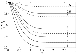
Figure 2: Evolution of fidelities $f_{0}(\tau)$ (solid curves) and $f_{1}(\tau)$ (dashed curves) are given by Eq. (57) for different values of intensity $|\alpha|^{2}$. It is seen that the curves for $f_{0}(\tau)$ and $f_{1}(\tau)$ coincide if $|\alpha|^{2}\geq 4$.

We can also study the effect of the phase damping on the entangled qubit (28) based on the above discussions, and the relevant calculations are straightforward. Here, we only give a fidelity $F(t)$ for two modes subjected to the phase damping as

$$F(\tau) = \frac{1}{2}f_{0}(\tau)f_{1}(\tau)+\frac{2e^{-\tau^{2}}}{{\rm sh}^{2}(2|\alpha|^{2})}$$

$$\times\left(\sum_{n,m}\frac{|\alpha|^{2(2n+2m+1)}e^{-2(n-m)(n-m+1)\tau^{2}}}{(2m)!(2n+1)!}\right)^{2}$$

where $f_{0}(\tau)$ and $f_{1}(\tau)$ are given by Eq. (57). Assuming that both channels have the same phase damping constant $\Gamma$. Eq. (III.2) simplifies to the following single-sum formula

$$F(\tau) = \frac{1}{2}f_{0}(\tau)f_{1}(\tau)+\frac{2e^{-\tau^{2}}}{{\rm sh}^{2}{(2|\alpha|^{2})}}$$

$$\times\left(\sum_{d=1}^{\infty}e^{-2d(d+1)\tau^{2}}I_{2d+1}(2{|\alpha|^{2}})+I_{1}(2{|\alpha|^{2}})\right)^{2}$$

which helps us to find approximate compact-form solutions. E.g., for either long scaled interaction times, $\tau\gg 1$, or low intensities, $|\alpha|^{2}\ll 1$, the fidelity $F(\tau)$ reduces to

$$F(\tau)\approx\frac{1}{2}f_{0}(\tau)f_{1}(\tau)+\frac{2e^{-\tau^{2}}}{{\rm sh}^{2}{(2|\alpha|^{2})}}[I_{1}(2{|\alpha|^{2}})]^{2}.$$ (63)

On the other hand, by assuming high intensity, $\ {|\alpha|^{2}}\gg 1$, together with $\tau\gg 1$, one obtains the following approximation

$$F(\tau)\approx\frac{1}{2\pi{|\alpha|^{2}}}\left[1+4\exp(-\tau^{2})\right].$$ (64)

If the qubit states are defined by the vacuum state $|0\rangle$ as logical zero state and single-photon state $|1\rangle$ as logical one state, then for the entangled qubits (36), if both of them go into phase damping channels with the same damping constant $\Gamma$, we can obtain the fidelity as

$$F^{\prime}(\tau)=\frac{1}{2}\left\{1+e^{-\tau^{2}}\right\}.$$ (65)

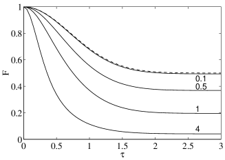
Figure 3: Evolution of fidelities $F^{\prime}(\tau)$ (dashed curve), given by Eq. (65), and $F(\tau)$ (solid curves), given by Eq. (III.2), for different values of intensity $|\alpha|^{2}$.

In Fig.(3), we compare the fidelities for the Eqs.(III.2) (65). We find that their fidelities are almost the same when the odd and even coherent qubit states are in the low intensity limit. But when the intensity increases, the fidelity given in Eq.(III.2) is less than that in Eq.(65). It shows that in case of the phase damping, the odd and even coherent states are not good coding states.

IV conclusions and discussions

Using a simple operator algebra solution, we have derived the Kraus representation of a harmonic oscillator suffering from the zero temperature environmental effect, which is modeled as the amplitude damping or the phase damping. It is worth noting that we could not derive a compact form for the Kraus representation when the environment is initially in the thermal field, because it becomes very difficult to distinguish the number of photons detected by the environment and that absorbed by the system due to the existence of the thermal field, which can excite the system to higher states last .

As examples and applications of a system in a zero temperature environment, we first give a Kraus representation of a single qubit whose computational basis states are defined as bosonic vacuum and single particle number states. We further discuss the environment effect on the qubits whose computational basis states are defined as the bosonic odd and even coherent states. We find that when the system suffers from the amplitude damping, the loss of even number of photons leaves the qubit, whose computational basis is defined by the even and odd coherent states, unchanged, but the loss of an odd number of photons changes the even or odd properties of the qubit. If the system loses a few photons and the intensity of the coherent states is taken infinitely large, then we can roughly say that the loss of an even number of photons keeps qubit unchanged, but the loss of an odd number of photons causes a bit flip error. Such an error can be corrected by some unitary operation. But if the computational basis is defined by the vacuum and single-photon states, a single-photon loss is an irreversible process, we cannot find any unitary operation to correct this error resulting from a single photon loss. So in the amplitude damping channel, the use of the even and odd coherent states as logical qubit is more suitable than the use of the vacuum and single-photon state as logical states ptc ; oliver .

When the qubit states, whose computational basis is defined by the even and odd coherent states, enter the phase damping channels, the even and odd properties will not be changed, however all off-diagonal terms of the qubit density matrices gradually vanish. Then the originally pure states change into mixtures of states because of the random scattering of the environment on the system even without loss of photons. It is much more difficult to correct such an error. So the use of the even and odd coherent states as logical qubit states cannot solve the problem of the phase damping.

V acknowledgments

Yu-xi Liu thanks Franco Nori for his helpful discussions. Yu-xi Liu was supported by the Japan Society for the Promotion of Science (JSPS). This work is partially supported by a Grant-in-Aid for Scientific Research (C) (15340133) by the Japan Society for the Promotion of Science (JSPS).

References

- (1) K. Kraus, State, Effects, and Operations (Springer, Berlin, 1983); Ann. Phys. 64, 311 (1971).
- (2) M.A. Nielsen and I.L. Chuang, Quantum Computation and Quantum Infromation (Cambridge University Press, Cambridge, 2000).
- (3) B. Schumacher, Phys. Rev. A 54, 2614 (1996).
- (4) M.A. Nielsen and C.M. Caves, Phys. Rev. A 55, 2547 (1997).
- (5) D.A. Lidar, Z. Bihary, and K.B. Whaley, Chemical Phys. 268, 35 (2001); D. Bacon, D.A. Lidar, and K.B. Whaley, Phys. Rev. A 60, 1944 (1999).
- (6) P. Stelmachovic and V. Bužek, Phys. Rev. A 64, 062106 (2001); H. Hayashi, G. Kimura, Y. Ota, Phys. Rev. A 67, 062109 (2003); P. Caban, K.A. Smoliński, and Z. Walczak, Phys. Rev. A 68, 034308 (2003); D.M. Tong, L.C. Kwek, C.H. Oh, J.L. Chen, and L. Ma, Phys. Rev. A 69, 054102 (2004).
- (7) I.L. Chuang, D.W. Leung, and Y. Yamamoto, Phys. Rev. A 56, 1114 (1997).
- (8) G.J. Milburn, Proceedings of the Fifth Physics Summer School, 435-465, Atomic and Molecular Physics and Quantum Optics, edited by H-A. Bachor, et al.(World Scientific, Singapore, 1992); D. Vitali, P. Tombesi, and G.J. Milburn, Phys. Rev. A 57, 4930 (1998).
- (9) W.H. Louisell, Quantum Statistical Properties of Radiation, (John Wiley & Sons, New York, 1973).
- (10) C.P. Sun, Y.B. Gao, H.F. Dong, and S.R. Zhao, Phys. Rev. E 57, 3900 (1998).
- (11) M. Brune, E. Hagley, J. Dreyer, X. Maître, A. Maali, C. Wunderlich, J.M. Raimond, and S. Haroche , Phys. Rev. Lett. 77, 4887 (1996); C. Monroe, D.M. Meekhof, B.E. King, D.J. Wineland, Science 272, 1131 (1996).
- (12) P.T. Cochrane, G.J.Milburn, and W.J. Munro, Phys. Rev. A 59, 2631 (1999).
- (13) M.C. de Oliveira and W.J. Munro, Phys. Rev. A61, 042309 (2000).
- (14) V. Peřinová and A. Lukš, Phys. Rev. A 41, 414 (1990); Q.A. Turchette, C.J. Myatt, B.E. King, C.A. Sackett, D. Kielpinski, W.M. Itano, C. Monroe, and D.J. Wineland, Phys. Rev. A 62, 053807 (2000); A. Miranowicz and W. Leoński, J. Opt. B 6, 43 (2004).