Teleportation of an atomic ensemble quantum state

Abstract

We propose a protocol to achieve high fidelity quantum state teleportation of a macroscopic atomic ensemble using a pair of quantum-correlated atomic ensembles. We show how to prepare this pair of ensembles using quasiperfect quantum state transfer processes between light and atoms. Our protocol relies on optical joint measurements of the atomic ensemble states and magnetic feedback reconstruction.

The realization of quantum networks involving optical fields and atomic ensembles is one of the most promising path towards robust long distance quantum communication and information processing chuang ; zoller . The efficient transfer of quantum states within that network is a key ingredient for a practical implementation zoller . Several continuous variable teleportation experiments with optical fields furusawa have shown that continuously teleporting optical quantum states with a high efficiency was possible. On the other hand the teleportation of a single atom or ion quantum state was demonstrated very recently wineland . In this Letter we present a direct scheme to teleport an atomic spin state in a way very similar to that used in the teleportation protocols for optical field states kimble , which can hence be efficiently integrated within a light-atom quantum network, for instance.

Because of the long lifetime of their ground state spins atomic ensembles are good candidates to store and manipulate quantum states of light lukin . We base ourselves on proposals predicting quasiperfect quantum state transfer between field and atoms dantan1 ; dantan3 ; dantan4 and propose to achieve the teleportation of an atomic ensemble (1) quantum state using an Einstein-Podolsky-Rosen-correlated pair of atomic ensembles (2) and (3). An optical joint measurement of the unknown ensemble 1 and one of the entangled ensemble 2 is then performed by Alice who sends the results to Bob. Using a suitable magnetic field Bob can reconstruct the input state on the other correlated ensemble 3. The quasiideal character of the atom-field quantum transfer processes allows high fidelity teleportation for easily accessible experimental parameters.

Another atomic teleportation protocol, relying on successive measurements alternating with optical displacements performed on two ensembles, was proposed by Kuzmich and Polzik kuzmich . However, this protocol requires several exchanges of information between Alice and Bob. Our scheme, being a direct adaptation of the teleportation protocols for light, needs two simultaneous measurements to achieve real-time quantum teleportation, and can easily be extended to other quantum communication and information protocols, such as entanglement swapping and quantum repeaters. This article successively describes the three steps of atomic teleportation : preparation, joint measurement and reconstruction.

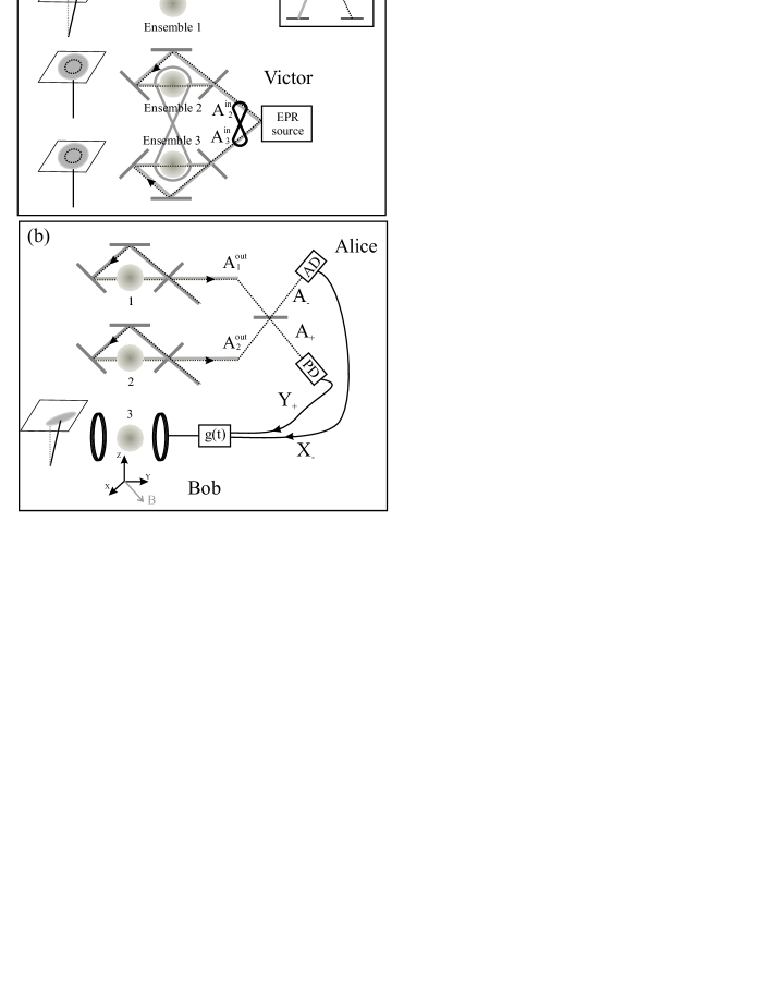
Figure 1: Teleportation scheme: (a) Preparation. Insert: $\Lambda$-type level structure considered. Left: schematic atomic initial states for each ensemble [for spins 2 and 3, the dashed circle indicates the coherent spin state fluctuation distribution]. (b) Measurement and reconstruction. Left: teleported state after reconstruction is completed. AD: amplitude detector. PD: phase detector.

Preparation. We consider three $N$-atoms atomic ensembles, labelled 1, 2, 3, with an energy level structure in $\Lambda$ [Fig. 1(a)]. We assume that they are placed inside optical cavities, for which the input-output theoretical treatment of the atom-field quantum fluctuations is well-adapted. They interact with a coherent control field $\Omega_{i}$ and with a vacuum field $A_{i}$. During the preparation stage Victor pumps the ensembles with the control fields, so that their ground state collective spins are aligned along the $z$-axis: $\langle J_{zi}\rangle=N/2$ ($i=1-3$). Ensemble 1 is assumed to be almost completely spin-polarized along $z$, with a small tilt corresponding to a non-zero coherence: $\langle J_{z1}\rangle\simeq N/2$ and $\langle J_{x1}\rangle,\langle J_{y1}\rangle\sim\mathcal{O}(\sqrt{N})$. This means that we consider small planar displacements of the spin in the vicinity of the north pole of the Bloch sphere. This approximation is all the more correct as the number of atoms is large. The quantum state of an ensemble is then determined by the ground state coherence, the spin components $J_{x}$ and $J_{y}$ obeying a commutation relation $\langle[J_{x},J_{y}]\rangle=i\langle J_{z}\rangle=iN/2$, similar to that of an harmonic oscillator. In the Gaussian approximation the atomic quantum state can then be represented by a noise ellipsoid in the $(x,y)$-plane orthogonal to the mean spin. It is then completely characterized by the coherence mean value and its variances $\Delta J_{x}^{2}$ and $\Delta J_{y}^{2}$, which are equal to $N/4$ for a coherent spin state for instance.

Let us suppose that the atomic state to be teleported is that of ensemble 1, prepared by Victor, unknown to Alice and Bob. With a suitable interaction dantan1 ; dantan3 Victor can prepare any Gaussian state (coherent state, squeezed state…) by an adequate choice of the field state $A_{1}^{in}$, the state of which can be perfectly mapped onto the atoms. More explicitly, the ”tilt” depends on the field intensity and phase, whereas the noise ellipsoid is given by the field quantum fluctuations dantan3 . Moreover, following a method detailed in dantan4 , Victor can also entangle ensembles 2 and 3 by transferring the quantum correlations from a pair of EPR-fields to the two spins. This can be achieved using an ”EIT” (one- and two-photon resonant) or a ”Raman” (large one-photon detuning, but two-photon resonant) interaction between the fields and the atoms. In these two configurations there is little to no dissipation and the quantum fluctuations are predicted to be conserved in atom-field quantum state transfer processes, but other situations to generate these EPR ensembles could also be envisaged polzik . Since the mean spins are parallel and equal, $J_{x2}-J_{x3}$ and $J_{y2}+J_{y3}$ are the equivalent of the usual EPR operators, satisfying $\langle[J_{x2}-J_{x3},J_{y2}+J_{y3}]\rangle=i\langle J_{z2}-J_{z3}\rangle=0$. We can assume without loss of generality that the fluctuations of $J_{x2}$ and $J_{x3}$ are correlated and those of $J_{y2}$ and $J_{y3}$ anti-correlated, so that the condition for their inseparability reads duan

$$\Delta(J_{x2}-J_{x3})^{2}+\Delta(J_{y2}+J_{y3})^{2}<|\langle J_{z2}\rangle|+|\langle J_{z3}\rangle|=N.$$

In a symmetrical configuration the amount of entanglement is given by the sum of the EPR variances (normalized to 2) giedke

$$\mathcal{I}_{2,3}=\frac{2}{N}[\Delta(J_{x2}-J_{x3})^{2}+\Delta(J_{y2}+J_{y3})^{2}].$$ (1)

When the preparation stage is over all fields are switched off, and one disposes of an unknown atomic quantum state 1 and an EPR-correlated pair 2 and 3.

Joint measurements. Alice then performs a simultaneous readout of ensembles 1 and 2 by rapidly switching on the control fields in cavities 1 and 2. As shown in dantan3 the states of spins 1 and 2 imprint in a transient manner onto the outgoing fields exiting the cavities $A_{1}^{out}$ and $A_{2}^{out}$. These two fields are then mixed on a 50/50 beamsplitter and Alice performs two homodyne detections of the resulting modes $A_{\pm}=(A_{1}^{out}\pm A_{2}^{out})/\sqrt{2}$ [Fig. 1(b)]. To obtain maximal information about the initial state, Alice measures the noise of two orthogonal quadratures - say $X_{-}=A_{-}+A_{-}^{\dagger}$ and $Y_{+}=i(A_{+}^{\dagger}-A_{+})$ - and sends the results to Bob who disposes of ensemble 3. As we will show further Bob can then reconstruct state 1 using a suitable magnetic field and achieve teleportation.

In more details, assuming one- and two-photon resonances (”EIT”-type interaction), Alice rapidly switches the control field on in ensembles 1 and 2 at $t=0$. The outgoing modes can be expressed as a function of the initial atomic operators in ensembles 1 and 2 dantan3

$$X_{i}^{out}(t) = X_{i}^{in}(t)-\alpha J_{xi}(0)e^{-\tilde{\gamma}_{0}t}$$

$$-2\eta^{2}[X_{i}^{in}(t)-\tilde{\gamma}_{0}\int_{0}^{t}e^{-\tilde{\gamma}_{0}(t-s)}X_{i}^{in}(s)ds]$$

$$+\beta[X_{vi}(t)-\tilde{\gamma}_{0}\int_{0}^{t}e^{-\tilde{\gamma}_{0}(t-s)}X_{vi}(s)ds],$$

($i=1,2$), with $\eta^{2}=2C/(1+2C)$, $\alpha=\eta\sqrt{8\tilde{\gamma}_{0}/N}$, $\beta=2\eta/\sqrt{1+2C}$, $C$ being the cooperativity parameter quantifying the collective strength of the atom-field coupling dantan1 . $\tilde{\gamma}_{0}$ represents the effective atomic decay rate in presence of the control field. This parameter depends on the cooperativity and the optimal pumping rate due to the control field dantan3 , and it is related to the duration of the transient optical pulse carrying the atomic state out of the cavity. $\eta$ is actually related to the efficiency of the transfer dantan1 , and is close to unity for large values of the cooperativity. $X_{vi}$ is a noise atomic operator accounting for noise induced by spontaneous emission and with unity white noise spectrum. $X_{i}^{in}$ is the amplitude quadrature of the vacuum field incident on cavity $i$. Similar expressions hold for the phase quadratures $Y_{i}$, replacing $x$’s, $X$’s by $y$’s, $Y$’s. To derive (Teleportation of an atomic ensemble quantum state) we assumed a cavity frequency bandwidth much larger than $\tilde{\gamma}_{0}$. In (Teleportation of an atomic ensemble quantum state) the amplitude of the term proportional to $J_{x}(0)$ shows how the atomic state reflects on the outgoing field state. The other terms correspond to intrinsic optical field noise ($\varpropto X^{in}$) and added atomic noise ($\varpropto X_{v}$). The photocurrents measured by Alice can be expressed as a sum of these noise terms and the atomic state:

$$i_{-} \varpropto X_{-}\sim noise+[J_{x1}(0)-J_{x2}(0)]e^{-\tilde{\gamma}_{0}t},$$ (3)

$$i_{+} \varpropto Y_{+}\sim noise+[J_{y1}(0)+J_{y2}(0)]e^{-\tilde{\gamma}_{0}t}.$$ (4)

By choosing the right temporal profile of her local oscillator it was shown in dantan3 that Alice can measure with a great efficiency the atomic states, which corresponds to the joint measurements used in the continuous variable teleportation protocols for light.

Reconstruction. From Alice’s results and his correlated ensemble 3 Bob is therefore in principle able to deduce the initial state of ensemble 1. Were we dealing with light beams Bob could directly feed Alice’s measurements to standard phase/intensity modulators to reconstruct state 1 kimble ; furusawa . The difficulty with an atomic ensemble is to physically implement the reconstruction stage. An all optical method was proposed in kuzmich . Another way to control the quantum fluctuations of an atomic ensemble is to use a magnetic field in order to have the spin precess in a controlled manner. Such a method was proposed to generate spin squeezing wiseman and was successfully implemented recently by Geremia et al. to continuously monitor the atomic spin noise via feedback geremia . We propose here to use a transverse magnetic field, the components of which are proportional to Alice’s homodyne detection results. Indeed, if we choose the components of the magnetic field, $B_{x}$ and $B_{y}$, to be proportional to $-i_{+}$ and $i_{-}$ we will couple $J_{x3}$ to $i_{-}$, and $J_{y3}$ to $i_{+}$. Since spin 2 and 3 are initially correlated, we intuitively expect their correlated noises to cancel leaving only spin 1 state imprinted onto that of spin 3 at the end of the reconstruction phase.

More quantitatively, the Hamiltonian corresponding to the unitary transformation that Bob performs on spin 3 is simply a $\vec{J}.\vec{B}$ coupling

$$H_{B}=-\lambda[B_{x}(t)J_{x3}+B_{y}(t)J_{y3}].$$ (5)

The evolution equations of $J_{x3}$ and $J_{y3}$ are then of the form

$$\dot{J}_{x3}(t)=G(t)X_{-}(t),\hskip 8.5359pt\dot{J}_{y3}(t)=G(t)Y_{+}(t),$$ (6)

in which $G(t)$ gives the electronic gain of the reconstruction process. Its temporal profile can be adjusted in order to maximize the fidelity of the reconstruction. At this point we would like to stress that choosing the right profile for this electronic gain is equivalent to choosing the right local oscillator profile in Alice’s homodyne detections. We therefore choose a temporal profile in $G(t)=Ge^{-\tilde{\gamma}_{0}t}$ for the gain, which we know will maximize the information that Bob gets dantan3 . After completion of the reconstruction, i.e. for $t\gg 1/\tilde{\gamma}_{0}$, the final state of $J_{x3}$, which we denote by $J_{x3}^{out}$, can be shown to be

$$J_{x3}^{out}=gJ_{x1}(0)+J_{x3}(0)-gJ_{x2}(0)+J_{x}^{\;noise}$$ (7)

in which $g=-G\eta/\sqrt{N\tilde{\gamma}_{0}}$ is the normalized gain of the teleportation protocol and $J_{x}^{\;noise}$ is a vacuum noise operator taking into account the losses of the process. Its explicit form is not reproduced, but it is uncorrelated with the spin operators and its variance, which can be calculated from Eqs. (Teleportation of an atomic ensemble quantum state) and (6), is related to the intrinsic noise added during the atom-field transfer processes: $\Delta^{2}J^{\;noise}_{x}=(N/2)g^{2}(1-\eta^{2})/\eta^{2}$.

We assume for simplicity initial isotropic fluctuations for the EPR-entangled ensembles, i.e. $\Delta J_{xi}^{2}=\Delta J_{yi}^{2}=(N/4)\cosh(2r)$ ($i=2,3$), and symmetrical correlations $\langle\delta J_{x2}\delta J_{x3}\rangle=-\langle\delta J_{y2}\delta J_{y3}\rangle=(N/4)\sinh(2r)$. With these notations the inseparability criterion value (1) is then given by $\mathcal{I}_{2,3}=2e^{-2r}$, which is 0 for perfect EPR entanglement and 2 for no entanglement. The normalized variance of $J_{x3}$, after reconstruction is then

$$V_{x3}^{out} = g^{2}V_{x1}+2g^{2}\frac{1-\eta^{2}}{\eta^{2}}$$ (8)

$$+(1+g^{2})\cosh(2r)-2g\sinh(2r),$$

with an identical expression for the variance of $J_{y3}$. Note that, if the gain is set to 0, one retrieves the fact that the fluctuations of spin 3 are not modified: $V_{x3}^{out}=\cosh(2r)=V_{x3}$. Setting a unity gain ($g=1$), the variances of the equivalent input noises $N_{\alpha}^{out}\equiv V_{\alpha 3}^{out}-g^{2}V_{\alpha 1}$ ($\alpha=x,y$) grangier are related to the EPR entanglement and the losses

$$N_{x,y}^{out}=2e^{-2r}+2\frac{1-\eta^{2}}{\eta^{2}}.$$ (9)

For high entanglement ($r\gg 1$) and negligible losses ($\eta\sim 1$) the equivalent input noises go to 0, which means that the state of spin 1 have indeed been fully teleported to spin 3.

At this point we can make a few comments. First, this result is very similar to that of light beam teleportation protocols furusawa ; kimble ; grangier ; treps and shows that the input noise variances go down to 0 if Alice and Bob share perfectly entangled ensembles ($r=\infty$) and in the absence of losses ($\eta=1$). In absence of entanglement ($r=0$), $N_{x}^{out}=N_{y}^{out}=2$, one retrieves the fact that two units of vacuum noise are added for the measurement and the reconstruction in the protocol. A good criterion to estimate the quality of the teleportation is provided by the product of the equivalent input noise variances $V_{q}\equiv\sqrt{N_{x}^{out}N_{y}^{out}}$ treps . In the absence of losses the classical limit of 2 is beaten as soon as one disposes of entanglement. The equivalent input noises being independent of the input state our teleportation protocol is unconditional. One should note that this is true in the ”small tilting” approximation limit ; the ”signal”, i.e. the mean value of spin 1 ground state coherence, has to be of the same order of magnitude as the fluctuations of the spin: $\langle J_{x1}\rangle,\langle J_{y1}\rangle\sim\mathcal{O}(\sqrt{N})$. Within this approximation the various measures used in light teleportation protocols furusawa ; kimble ; grangier to assess the success of the teleportation are valid. The non-unity gain situation can be analyzed using T-V diagrams or other measures treps .

Secondly, we have assumed that the measurement and the feedback times are negligible with respect to the ground state spin lifetime, so that ensemble 3 does not evolve before the reconstruction. This approximation is fairly reasonable since the ground state lifetime for cold atoms or paraffin-coated cells is at least of the order of several milliseconds or even up to the second kuzmich .

Third, the intrinsic noise ($\varpropto 1/C$), that is, the noise which does not come from the detector quantum inefficiency or electronic noise, is expected to be rather small, thanks to the cooperative behavior of the atoms in the cavity - $C$ can easily be made of the order of 100-1000 using low finesse cavities. This should ensure losses at the percent level and, therefore, a good teleportation. High-Q cavities are not required because the atom-field coupling is enhanced by the collective atomic behavior ($C\varpropto N$). Bad cavities are actually preferable since the cavity bandwidth has to be much larger than the atomic spectrum width $\tilde{\gamma}_{0}$.

It is also interesting to look at the physical meaning of the magnetic reconstruction. The unity gain condition $g=1$ actually translates into the very intuitive condition that the rotation angle of spin 3 during reconstruction in a time $(2\tilde{\gamma}_{0})^{-1}$ should be equal to the relative spin fluctuations: $\theta=\omega_{L}/(2\tilde{\gamma}_{0})=1/\sqrt{N}$, where $\omega_{L}$ is the Larmor frequency. This condition also gives us the order of magnitude of the magnetic field necessary to perform the reconstruction. For an interaction with $N=10^{6}$ cesium atoms on the $D_{2}$ line, a gyromagnetic factor of $450$ kHz/G and $\tilde{\gamma}_{0}=(2\pi)\;225$ kHz, the amplitude of the magnetic field is about $1$ mG.

Last, in order to check the quality of the teleportation Victor can simply perform a readout of ensemble 3 with the same technique previously used by Alice and compare the output state with the input state that he had prepared. Another way to check that this teleportation scheme is successful would be for Bob not to reconstruct the atomic state, but, instead, to perform an optical readout of ensemble 3 and use both his homodyne detection results and Alice’s results to deduce the input state. However, in this scheme, the atomic state of 1 is never effectively teleported to ensemble 3. The spin 1 state is actually teleported to the outgoing field $A_{3}^{out}$, realizing atom-to-field teleportation.

A straightforward, but nonetheless important application of our protocol for quantum communication is atomic entanglement swapping: if ensemble 1 in the previous scheme was initially quantum correlated with another ensemble 0, the previous teleportation scheme ensures that ensembles 0 and 3 are entangled at the end of the process. This is of importance for the realization of quantum networks in which quantum repeaters can ensure good quality transmission of the quantum information over long distances zoller .

^∗Electronic address: dantan@spectro.jussieu.fr

References

- (1) M. Nielsen and I. Chuang, Quantum computation and quantum information (Cambridge University Press, 2000).
- (2) L.M. Duan, J.I. Cirac, P. Zoller and E.S. Polzik, Phys. Rev. Lett. 85, 5643 (2000); L.M. Duan et al., Nature (London) 414, 413, (2001).
- (3) A. Furusawa et al., Science 282, 706 (1998); W.P. Bowen et al., Phys. Rev. A 67, 032302 (2003); T.C. Zhang et al., Phys. Rev. A 67, 033802 (2003).
- (4) M. Riebe et al., Nature (London) 429, 734 (2004); M.D. Barrett et al., Nature (London) 429, 737 (2004).
- (5) M.D. Lukin, Rev. Mod. Phys. 75, 457 (2003).
- (6) S.L. Braunstein and H.J. Kimble, Phys. Rev. Lett. 80, 869 (1998).
- (7) A. Dantan et al., Phys. Rev. A 67, 045801 (2003).
- (8) A. Dantan and M. Pinard, Phys. Rev. A 69, 043810 (2004).
- (9) A. Dantan, A. Bramati and M. Pinard, Europhys. Lett. to be published, quant-ph/0405020 (2004).
- (10) A. Kuzmich and E.S. Polzik, Phys. Rev. Lett. 85, 5639 (2000).
- (11) B. Julsgaard, A. Kozekhin and E.S. Polzik, Nature (London) 413, 400 (2001).
- (12) L.M. Duan et al., Phys. Rev. Lett. 84, 2722 (2000); R. Simon, Phys. Rev. Lett. 84, 2726 (2000).
- (13) G. Giedke et al., Phys. Rev. Lett. 91, 107901 (2003).
- (14) T.C Ralph and P.K. Lam, Phys. Rev. Lett. 81, 5668 (1998); F. Grosshans and P. Grangier, Phys. Rev. A 64, 010301 (2001).
- (15) L.K. Thomsen, S. Mancini and H.M. Wiseman, Phys. Rev. A 65, 061801 (2002).
- (16) J.M. Geremia, J.K. Stockton and H. Mabuchi, Science 304, 270 (2004).
- (17) W.P. Bowen et al., IEEE Journal of Selected topics in Quantum Electronics 9, 1519 (2003).