Theory of decoherence in a matter wave Talbot-Lau interferometer

Abstract

We present a theoretical framework to describe the effects of decoherence on matter waves in Talbot-Lau interferometry. Using a Wigner description of the stationary beam the loss of interference contrast can be calculated in closed form. The formulation includes both the decohering coupling to the environment and the coherent interaction with the grating walls. It facilitates the quantitative distinction of genuine quantum interference from the expectations of classical mechanics. We provide realistic microscopic descriptions of the experimentally relevant interactions in terms of the bulk properties of the particles and show that the treatment is equivalent to solving the corresponding master equation in paraxial approximation.

I Introduction

The art of demonstrating the wave nature of material particles experienced considerable advances in recent years; see Berman (1997); Rauch and Werner (2000); Martellucci et al. (2000) and references therein. The interfering species evolved from the elementary particles of the early experiments Davisson and Germer (1927); Halban Jnr and Preiswerk (1936) to composite objects with an internal structure. In particular, the experiments in atom interferometry have left the stage of proof-of-principle demonstrations, and provide substantial applications in metrology Weiss et al. (1993); Ekstrom et al. (1995); Gustavson et al. (1997); Peters et al. (1999). Objects with even larger complexity, such as molecules or clusters, exhibit a rich internal structure that can interact in various ways with external fields. Their interference is highly sensitive to the corresponding phase shifts, thus offering the potential to measure molecular properties with unprecedented precision. At the same time any coupling to uncontrollable fields and environmental degrees of freedom severely limits the ability of large objects to show interference. These effects are bound to become dominant as the chosen objects increase in size and complexity.

The influence of environmental coupling on a quantum system may be described by decoherence theory Joos et al. (2003); Zurek (2003). It considers both the influence of noise due to uncontrollable external fields and the effect of the entanglement with unobserved dynamic degrees of freedom. This latter phenomenon – the dynamic delocalization of quantum coherence into many environmental degrees of freedom – largely explains the emergence of classical behavior in a quantum description. In particular, it describes the wave-particle complementarity encountered if one seeks to determine by a (macroscopic) measurement device the path taken. Since matter wave interferometers establish quantum coherence on a macroscopic scale they are sensitive tools to probe the quantum-to-classical transition of complex objects.

The purpose of this article is to provide the theoretical framework needed to describe the diffraction and decoherence effects encountered in the interferometry of large, massive objects. We focus on near-field Talbot-Lau interference, which is the favored setup for short de Broglie wavelengths. We take care to describe the effects of diffraction and decoherence with realistic parameters, to permit a direct quantitative comparison with the experimental signal. The interactions are treated on a microscopic level using the bulk properties of materials and particles. We note that the recent interference experiments with fullerenes and biomolecules Brezger et al. (2002); Hornberger et al. (2003); Hackermüller et al. (2003a, 2004) were analyzed using the theory presented in this article.

Before going into calculations we start with an informal discussion of Talbot-Lau interference Clauser and Li (1994a); Chapman et al. (1995a); Nowak et al. (1997). In this setup an essentially uncollimated particle beam passes three parallel gratings. Effectively, the first grating acts as an array of collimation slits which illuminate the second grating. Diffraction at the second grating then leads, for particular choices of the grating periods and the wavelength, to a high contrast near-field interference pattern at the position of the third grating. This density pattern is observed with the help of the third grating by recording the transmitted flux as a function of the lateral grating position.

An important advantage of the Talbot-Lau effect is the favorable scaling behavior with respect to larger masses of the interfering object Clauser (1997). Unlike in far-field diffraction, where the required grating period falls linearly with the de Broglie wavelength, it decreases merely like the square root in the Talbot-Lau setup. In addition, the collimation requirements are much weaker than for far field diffraction, and the spatially resolving detector is already built into the device.

However, for a fixed particle velocity it is not immediately evident whether the observed signal proves genuine quantum interference, since a certain fringe pattern could also be expected from a classical moiré effect. This classical pattern can be suppressed by an appropriate choice of the open fraction of the grating and, unlike the strong wave-length dependence found in the interference effect, the ideal classical shadow fringes do not depend on the velocity. Nonetheless, in order to distinguish clearly the quantum phenomenon from a classical expectation it is necessary to describe the quantum and the classical evolution in the same theoretical framework, thus ensuring that all interactions and approximations are treated equally.

A first aim of this article is to provide such a description that draws the demarcation line between the predictions of quantum and classical mechanics concisely and quantitatively. The second aim is then to account for the relevant environmental interactions, thus providing a quantitative description of the transition from the quantum to the classical behavior. For both goals it will be helpful to describe the state in the interferometer in terms of a stationary, unnormalized Wigner function. Due to the stationary formulation the effect of decoherence will not be given by a master equation. Therfore, it is shown in the final part of the paper that our treatment is equivalent to the conventional dynamic formulation of decoherence in terms of a normalized Wigner function.

The structure of the article is as follows: In Sect. II we review the coherent Talbot-Lau effect and give a formulation in terms of the Wigner function. The corresponding classical shadow effect is calculated on an equal footing in the phase space representation. The influence of the interaction with realistic gratings, which is very important for a quantitative description, is accounted for in Sect. III. Those effects are also treated on an equal degree of approximation in the quantum and the classical description. In Sect. IV we include the possibility of decoherence and show how it can be accounted for analytically. The specific predictions for decoherence due to collisions and due to heat radiation are then obtained in Sect. V. In Sect. VI we relate the description of decoherence in terms of a stationary beam to the solution of the corresponding time-dependent master equation. Concluding remarks are given in Sect. VII.

II The Talbot-Lau effect in the Wigner representation

Since the coherent theory of the Talbot-Lau effect can be found in the literature Talbot (1836); Patorski (1989); Dubetsky and Berman (1997); Brezger et al. (2003) we shall present no detailed derivations, but discuss the approximations involved and state the results in terms of the Wigner function as far as needed for the later inclusion of decoherence effects. Consider the usual interferometric situation where a flux of particles enters at $z=0$ with a longitudinal momentum $p_{z}$ that is much greater than its transverse components. Ideally, the particle is in a momentum eigenstate, or in an incoherent mixture thereof, before passing a number of collimation slits and gratings. The vector $\mathbf{r}=\left(x,y\right)$ describes the distance of the particles from the interferometer axis. In the usual paraxial approximation this separation, as well as the structures in the grating and in the collimation planes, are assumed to be small compared to the distances $L_{i}$ between the optical elements, $|\mathbf{r}|\ll L_{i}$. In this case one may evaluate the transmission to leading order in $|\mathbf{r}|/L_{i}$. This approximation implies that the longitudinal and the transverse part of the state remain separable throughout the interferometer. It follows that the discussion may be confined to the transverse degrees of freedom as described by $\psi(\mathbf{r})$ if the evolution is completely coherent — or, in the general case, by the density matrix $\rho(\mathbf{r},\mathbf{r}^{\prime})$.

Given the wave function $\psi_{0}(\mathbf{r})$ on the $z=0$ plane the free unitary evolution up to the plane $z=L$ yields, to leading order, the transverse state,

$$\psi_{L}(\mathbf{r})=\frac{p_{z}}{2\pi\hbar\mathrm{i}L}\,\mathrm{e}^{\mathrm{i}p_{z}L/\hbar}\int\mathrm{d}\mathbf{r}_{0}\,\exp\!\left(\mathrm{i}\frac{p_{z}}{\hbar}\frac{|\mathbf{r}-\mathbf{r}_{0}|^{2}}{2L}\right)\psi_{0}(\mathbf{r}_{0})\,+{\mathcal{O}}\left(\frac{\mathbf{r}^{2}}{L^{2}}\right)\;,$$ (1)

as follows from an asymptotic expansion of the free Green function, e.g. Sommerfeld (1950). An important feature of this paraxial approximation is the fact that it reflects the composition property of the exact propagation without any loss of accuracy. That is, propagating the wave function first by a distance $L_{1}$ and subsequently by the distance $L_{2}$ yields exactly the same result as a single propagation by $L_{1}+L_{2}$,

$$\psi_{3}(\mathbf{r}_{3})= -\frac{p_{z}^{2}}{\left(2\pi\hbar\right)^{2}L_{1}L_{2}}\,\mathrm{e}^{\mathrm{i}\left(p_{z}L_{1}+p_{z}L_{2}\right)/\hbar}\int\mathrm{d}\mathbf{r}_{1}\mathrm{d}\mathbf{r}_{2}\,\exp\!\left(\mathrm{i}\frac{p_{z}}{\hbar}\frac{|\mathbf{r}_{3}-\mathbf{r}_{2}|^{2}}{2L_{2}}\right)\exp\!\left(\mathrm{i}\frac{p_{z}}{\hbar}\frac{|\mathbf{r}_{2}-\mathbf{r}_{1}|^{2}}{2L_{1}}\right)\psi_{1}(\mathbf{r}_{1})$$

$$= \frac{p_{z}}{2\pi\hbar\mathrm{i}(L_{1}+L_{2})}\,\mathrm{e}^{\mathrm{i}p_{z}(L_{1}+L_{2})/\hbar}\int\mathrm{d}\mathbf{r}_{1}\,\exp\!\left(\mathrm{i}\frac{p_{z}}{\hbar}\frac{|\mathbf{r}_{1}-\mathbf{r}_{3}|^{2}}{2(L_{1}+L_{2})}\right)\psi_{1}(\mathbf{r}_{1})\;,$$ (2)

which follows from Gaussian integration. Hence, within the paraxial approximation no loss of accuracy is introduced by dividing the propagation into a sequence of intervals and integrating over the interjacent planes. This freedom will be used below as a crucial ingredient when we describe the effects of decoherence.

Note that the composition property (2) does not require a large separation between the planes. Even for infinitesimally close planes one obtains the correct expression (1). This can be seen immediately in (2) by noting a particular representation of the two-dimensional $\delta$ function (Hornberger and Smilansky, 2002, eq. (A.33)),

$$\frac{p_{z}}{2\pi\hbar\mathrm{i}L}\exp\!\left(\mathrm{i}\frac{p_{z}}{\hbar}\frac{|\mathbf{r}-\mathbf{r}_{0}|^{2}}{2L}\right)\begin{CD}@>{\hbar L/p_{z}\to 0}>{}>\delta_{2}(\mathbf{r}-\mathbf{r}_{0})\end{CD}\;.$$ (3)

The first equality in (2) also shows how the existence of an ideal grating at $z=L_{1}$ would affect the propagated state. In the case of a binary grating the $\mathbf{r}_{2}$-integration would be simply restricted to the transparent parts of the grating plane. In general, an ideal grating causes an amplitude and phase modulation

$$\psi_{1}^{\prime}(\mathbf{r}_{2})=t(\mathbf{r}_{2})\psi_{1}(\mathbf{r}_{2})\quad\text{with}\quad|t(\mathbf{r}_{2})|<1\;,$$ (4)

which is accounted for by the additional appearance of a grating function $t(\mathbf{r}_{2})$ under the integral.

The passage of a particle stream through a general interferometer may now be described as a sequence of transmissions through gratings or collimation slits as described by (4) each followed by a free evolution (1). This holds also for general, mixed states since any density operator can be represented as a convex sum of projectors to pure states.

II.1 Wigner function

We proceed to formulate the propagation in the Wigner representation, which has several advantages. First, the Wigner function permits a direct comparison of the quantum evolution to the classical dynamics in terms of phase space distributions. Second, and more importantly, it is the most convenient starting point to include effects of decoherence in Sect. IV. Finally, the free evolution (1) has a particularly simple form in the Wigner representation.

The Wigner function is the Fourier transformation of the position density matrix $\rho(\mathbf{r},\mathbf{r}^{\prime})$ with respect to the two-point separation $\boldsymbol{\Delta}=\mathbf{r}-\mathbf{r}^{\prime}$ Wigner (1932),

$$w(\mathbf{r},\mathbf{p})=\frac{1}{(2\pi\hbar)^{2}}\int\mathrm{d}\boldsymbol{\Delta}\,\mathrm{e}^{\mathrm{i}\mathbf{p}\boldsymbol{\Delta/}\hbar}\rho\left(\mathbf{r}-\frac{\boldsymbol{\Delta}}{2},\mathbf{r}+\frac{\boldsymbol{\Delta}}{2}\right)\;.$$ (5)

It may be viewed as a quantum analogue to the classical phase space distribution $f(\mathbf{r},\mathbf{p})$, with $\mathbf{p}$ the transverse momentum vector.

In order to obtain the free unitary evolution of the Wigner function we note that the density matrix in position representation has the general form

$$\rho(\mathbf{r},\mathbf{r}^{\prime})=\int\mathrm{d}\mu\,g(\mu)\psi_{\mu}(\mathbf{r})\psi_{\mu}^{\ast}(\mathbf{r}^{\prime})$$ (6)

with $\int\mathrm{d}\mu\,g(\mu)=1$. According to (1) a free unitary evolution by the distance $L$ yields

$$\rho(\mathbf{r},\mathbf{r}^{\prime})=\frac{p_{z}^{2}}{\left(2\pi\hbar\right)^{2}L^{2}}$$

$$\times\int\mathrm{d}\mathbf{r}_{0}\mathrm{d}\mathbf{r}_{0}^{\prime}\,\exp\!\left(\mathrm{i}\frac{p_{z}}{\hbar}\frac{|\mathbf{r}-\mathbf{r}_{0}|^{2}-|\mathbf{r}^{\prime}-\mathbf{r}_{0}^{\prime}|^{2}}{2L}\right)\rho_{0}(\mathbf{r}_{0},\mathbf{r}_{0}^{\prime})\;.$$ (7)

From (5) and (7) it follows that a free unitary evolution by the distance $L$ changes the Wigner function according to

$$w_{L}(\mathbf{r},\mathbf{p})=w_{0}\left(\mathbf{r}-\frac{L}{p_{z}}\mathbf{p},\mathbf{p}\right)\;.$$ (8)

This transformation is particularly simple and, as one expects, is identical to the free movement of a classical probability density in the phase space of the transverse degree of freedom. The decisive difference between the classical and the quantum phase space dynamics is found in the transformation for passing through a grating. Equation (4) implies that by going through a grating the Wigner function undergoes a convolution

$$w^{\prime}(\mathbf{r},\mathbf{p})=\int\mathrm{d}\mathbf{q}\,T(\mathbf{r},\mathbf{q})w(\mathbf{r},\mathbf{p}-\mathbf{q})$$ (9)

which in general builds up quantum coherences that show up as oscillations in the momentum direction. Here we define the convolution kernel analogously to (5) as

$$T(\mathbf{r},\mathbf{p})=\frac{1}{(2\pi\hbar)^{2}}\int\mathrm{d}\boldsymbol{\Delta}\,\mathrm{e}^{\mathrm{i}\mathbf{p}\boldsymbol{\Delta/}\hbar}t\left(\mathbf{r}-\frac{\boldsymbol{\Delta}}{2}\right)t^{\ast}\left(\mathbf{r}+\frac{\boldsymbol{\Delta}}{2}\right)\;.$$ (10)

Note that by stating (9) we do not keep the normalization of the Wigner function. Indeed, a finite fraction of the particles may hit the grating and may be removed from the flux. Therefore it is convenient to work with an unnormalized state and take care of the normalization only in the end.

With the transformations (8) and (9) we can proceed to describe the Talbot-Lau effect in a general framework.

II.2 The Talbot-Lau setup

In the Talbot-Lau setup a monochromatic beam passes three vertical gratings that are separated by the distances $L_{1}$ and $L_{2}$. Since the particle stream is effectively uncollimated in front of the first grating its Wigner function for the transverse degrees of freedom is uniform. If we start with the (improper) normalization $w_{0}(\mathbf{r},\mathbf{p})=1$ then (10) yields the Wigner function after the first grating

$$w_{1}(\mathbf{r},\mathbf{p})=|t_{1}(\mathbf{r})|^{2}\;.$$ (11)

The free unitary evolution by a distance $L_{1}$, followed by a passage through a grating (with convolution kernel $T$) and another free evolution by a distance $L_{2},$ leads to the general expression

$$w(\mathbf{r},\mathbf{p})=\,\int\mathrm{d}\mathbf{q}\,\left|t_{1}\left(\mathbf{r}-\frac{\mathbf{p}}{p_{z}}(L_{1}+L_{2})+\frac{\mathbf{q}}{p_{z}}L_{1}\right)\right|^{2}\\ \times T\left(\mathbf{r}-\frac{\mathbf{p}}{p_{z}}L_{2}\,,\mathbf{q}\right)\;.$$ (12)

The particle density at position $z=L_{1}+L_{2}$ is obtained by integrating the momentum variable. It can be written as

$$w(\mathbf{r})\equiv\,\int w(\mathbf{r},\mathbf{p})\,\mathrm{d}\mathbf{p}=\int\mathrm{d}\mathbf{r}_{1}\,|t_{1}(\mathbf{r}_{1})|^{2}\,h(\mathbf{r};\mathbf{r}_{1})$$ (13)

with

$$h(\mathbf{r};\mathbf{r}_{1})=\left(\frac{p_{z}}{\hbar L_{1}}\right)^{2}\\ \times\int\mathrm{d}\mathbf{p}\,T\left(\mathbf{r}-\frac{\mathbf{p}}{p_{z}}L_{2}\,,\frac{L_{1}+L_{2}}{L_{1}}\mathbf{p}-\frac{\mathbf{r}-\mathbf{r}_{1}}{L_{1}}p_{z}\right)\;.$$ (14)

As mentioned above the Talbot-Lau effect operates in the near-field regime, where the fact that the gratings have a finite lateral extension does not play a role; it only affects the overall count rate. It is therefore permissible to describe the gratings by idealized functions that are periodic on an infinite plane. Moreover, since the setup is invariant with respect to changes in the vertical position, it is sufficient to consider the Wigner function and the grating transmissions only as a function of the “horizontal” coordinates $(r_{x},p_{x})\equiv(x,p)$, see Fig. 1.

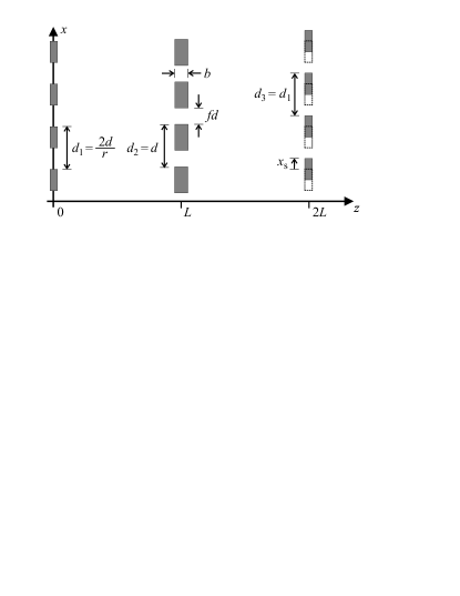
Figure 1: The symmetric Talbot-Lau setup consists of three parallel gratings separated by equal distances $L$. Near-field interference of an uncollimated beam from the left may lead to a density pattern at the position of the third grating that can be observed by modulation with the lateral grating position $x_{\mathrm{s}}.$

We take the first grating to have a period $d_{1}$, and its transmission function to be given by $t_{1}(x)=\sum a_{m}\exp(2\pi\mathrm{i}mx/d_{1})$. Likewise, the second grating has the Fourier coefficients $b_{m}$ and the period $d_{2}=d$. Therefore,

$$|t_{1}(x)|^{2}=\sum_{\ell\in\mathbb{Z}}A_{\ell}\exp\!\left(2\pi\mathrm{i}\ell\frac{x}{d_{1}}\right)\quad\text{with }A_{\ell}=\sum_{j\in\mathbb{Z}}a_{j}a_{j-\ell}^{\ast}$$ (15)

and

$$T(x,p)=\sum_{\ell,j\in\mathbb{Z}}b_{j}b_{j-\ell}^{\ast}\exp\!\left(2\pi\mathrm{i}\ell\frac{x}{d}\right)\delta\left(p-\hbar\pi\frac{2j-\ell}{d}\right).$$ (16)

In order to simplify the discussion and to avoid an overly complicated notation we focus on the symmetric Talbot-Lau setup, which is the most important one in practice; for the asymmetric setup see Brezger et al. (2003) and note . In this case the gratings are set at an equal distance $L_{1}=L_{2}\equiv L$ and the periods $d_{1}$ and $d$ of the first and second grating are related by $d_{1}=2d/r$, with $r\in\mathbb{N}$. (The case of equal grating periods, $r=2$, is most common Brezger et al. (2002); Hornberger et al. (2003); Hackermüller et al. (2003a, 2004).) The state (12) now reads

$$w(x,p)= \frac{1}{\hbar}\sum_{\ell,j,m\in\mathbb{Z}}A_{\ell}b_{j}b_{j-m}^{\ast}$$

$$\times\exp\!\left(2\pi\mathrm{i}\left(\frac{r}{2}\ell+m\right)\frac{x}{d}-2\pi\mathrm{i}(r\ell+m)\frac{L}{d}\frac{p}{p_{z}}\right)$$

$$\times\exp\!\left(\mathrm{i}\pi\ell(2j-m)\frac{r}{2}\frac{L}{{L_{\lambda}}}\right)\;.$$ (17)

Here we introduced the Talbot length

$${L_{\lambda}}=\frac{d^{2}p_{z}}{2\pi\hbar}=\frac{d^{2}}{\lambda}$$ (18)

in terms of the grating period $d$ and the de Broglie wavelength $\lambda=h/p_{z}.$ The Talbot length is the proper scale to distinguish near-field (Fresnel) diffraction from far-field (Fraunhofer) diffraction for a given wavelength. It gives the distance behind a grating where the diffraction peaks of a collimated, passing beam have a lateral separation equal to the grating period $d$.

To get the particle density in the beam from (II.2) we integrate over the momentum $p,$ which picks up the $m=-r\ell$ components ,

$$w(x)\equiv\int\mathrm{d}p\,w(x,p)\,\propto\,\sum_{\ell\in\mathbb{Z}}A_{\ell}^{\ast}B_{\ell r}^{(\lambda)}\exp\!\left(2\pi\mathrm{i}\ell\frac{x}{d_{1}}\right)$$ (19)

with Fourier components Brezger et al. (2003)

$$B_{m}^{(\lambda)}=\sum_{j\in\mathbb{Z}}b_{j}b_{j-m}^{\ast}\exp\!\left(\mathrm{i}\pi\frac{m^{2}-2jm}{2}\frac{L}{{L_{\lambda}}}\right)~{}.$$ (20)

Equation (19) predicts a density pattern which has the same period $d_{1}$ as the first grating. Often the spatial resolution of detectors is too poor to detect these density oscillations directly in an experiment. However, an indirect observation is possible with the help of a third grating with period $d_{1}$. If put at the position of the density pattern it modulates the total transmission as a function of its lateral position $x_{\mathrm{s}}$. The integrated transmission, which is much easier to detect, is then given by

$$S(x_{\mathrm{s}}) =\int\mathrm{d}p\,\mathrm{d}q\,\mathrm{d}x\,w(x,p-q)T(x-x_{\mathrm{s}},q)$$

$$=\int\mathrm{d}x\,w(x)|t_{3}(x-x_{\mathrm{s}})|^{2}\;.$$ (21)

If we choose the first and third grating to be identical, $t_{3}(x)=t_{1}(x)$, the expected periodic signal is given by the expression

$$S(x_{\mathrm{s}})\,\propto\,\sum_{\ell\in\mathbb{Z}}(A_{\ell}^{\ast})^{2}B_{\ell r}^{(\lambda)}\exp\!\left(2\pi\mathrm{i}\ell\frac{x_{\mathrm{s}}}{d_{1}}\right)\;.$$ (22)

For symmetric gratings this modulation signal has a visibility

$$\mathcal{V}_{\mathrm{qm}}=\frac{S_{\mathrm{max}}-S_{\mathrm{min}}}{S_{\mathrm{max}}+S_{\mathrm{min}}}=\frac{\left|\sum\limits_{n=1}^{\infty}A_{2n-1}^{2}B_{2nr-r}^{(\lambda)}\right|}{\frac{1}{2}A_{0}^{2}B_{0}^{(\lambda)}+\sum\limits_{n=1}^{\infty}A_{2n}^{2}B_{2nr}^{(\lambda)}}$$ (23)

which serves as the prime characterization of the interference pattern.

It is clear from the definition of the coefficients $B_{m}^{(\lambda)}$ that the interference pattern (19) and the visibility (23) depend strongly on both the wavelength $\lambda$ and on the separation $L$ between the gratings. As evident from (20) it is indeed the product of the two quantities which determines the pattern, since $L/{L_{\lambda}}=L\lambda/d^{2}$.

However, the detection of a periodic signal alone does not prove necessarily that quantum interference occurred in the experiment because a certain density pattern may also be expected from a generalized Moiré effect. To establish the observation of quantum interference one must show that the observed visibility differs significantly from the classical expectation. It is therefore important to have a reliable quantitative prediction for the classical expectation as well.

II.3 The classical expectation

With the results for the Wigner function at hand it is straightforward to repeat the calculation using classical phase space dynamics. The classical phase space density $f(\mathbf{r},\mathbf{p})$ transforms under free evolution like the Wigner function (8) according to

$$f_{L}(\mathbf{r},\mathbf{p})=f_{0}\left(\mathbf{r}-\frac{L}{p_{z}}\mathbf{p},\mathbf{p}\right)\;.$$ (24)

In contrast to (10), the convolution kernel for passing through an ideal amplitude grating is now given by

$$T_{\mathrm{cl}}(\mathbf{r},\mathbf{p})=\frac{1}{(2\pi\hbar)^{2}}\int\mathrm{d}\boldsymbol{\Delta}\,\mathrm{e}^{\mathrm{i}\mathbf{p}\boldsymbol{\Delta/}\hbar}|t(\mathbf{r})|^{2}=|t(\mathbf{r})|^{2}\delta(\mathbf{p})\;,$$ (25)

which leads to

$$f^{\prime}(\mathbf{r},\mathbf{p})=|t(\mathbf{r})|^{2}f(\mathbf{r},\mathbf{p})\;.$$ (26)

At a distance $L_{2}$ after the second grating this yields a phase space distribution

$$f(\mathbf{r},\mathbf{p})=\,\left|t_{1}\left(\mathbf{r}-\frac{\mathbf{p}}{p_{z}}(L_{1}+L_{2})\right)\right|^{2}\,\left|t_{2}\left(\mathbf{r}-\frac{\mathbf{p}}{p_{z}}L_{2}\right)\right|^{2}$$ (27)

which can also be obtained from the quantum result by replacing $T$ by $T_{\mathrm{cl}}$ in (12). It follows that the classical density pattern in front of the third grating is given by

$$f(x)\equiv\int\mathrm{d}p\,f(x,p)\,\propto\,\sum_{\ell\in\mathbb{Z}}A_{\ell}^{\ast}B_{\ell r}^{(0)}\exp\!\left(2\pi\mathrm{i}\ell\frac{x}{d_{1}}\right)$$ (28)

with

$$B_{m}^{(0)}=\sum_{j\in\mathbb{Z}}b_{j}b_{j-m}^{\ast}\;.$$ (29)

The comparison with (19) shows that the quantum and the classical results have the same form, but differ in the Fourier components $B_{m}$. Of course, the classical Fourier components do not depend on the de Broglie wavelength. Nonetheless, the $B_{m}^{(0)}$ may be viewed as the short-wave limit $L/{L_{\lambda}}\rightarrow 0$ of the quantum Fourier coefficients $B_{m}^{(\lambda)}$, which is already indicated by the notation.

It follows immediately that the classical prediction for the signal is obtained from (22) by replacing the wavelength dependent Fourier components $B_{m}^{(\lambda)}$ by the $B_{m}^{(0)}$,

$$S_{\text{cl}}(x_{\mathrm{s}})\,\propto\,\sum_{\ell\in\mathbb{Z}}(A_{\ell}^{\ast})^{2}B_{\ell r}^{(0)}\exp\!\left(2\pi\mathrm{i}\ell\frac{x_{\mathrm{s}}}{d_{1}}\right)\;.$$ (30)

Likewise one can show that the visibility of the classical signal is given, for symmetric gratings, by

$$\mathcal{V}_{\mathrm{cl}}=\frac{\left|\sum\limits_{n=1}^{\infty}A_{2n-1}^{2}B_{2nr-r}^{(0)}\right|}{\frac{1}{2}A_{0}^{2}B_{0}^{(0)}+\sum\limits_{n=1}^{\infty}A_{2n}^{2}B_{2nr}^{(0)}}\;.$$ (31)

Let us focus on the important case of equal grating periods for a moment, i.e., $r=2$. In this case only the even Fourier components $B_{2m}$ are needed. If the separation $L$ between the gratings is set to an integer multiple of the Talbot length, then it is easy to convince oneself that for any ideal grating $t_{2}(x)$

$$B_{2m}^{(\lambda)}=B_{2m}^{(0)}\qquad\text{if\ }\;L/{L_{\lambda}}\in\mathbb{N}$$ (32)

that is, the quantum and the classical evolution yield identical predictions for the density pattern and the observed visibility. This shows clearly that the observation of the integer Talbot-Lau effect alone does not prove the wave nature of the beam particles.

However, unlike their classical counterparts, the quantum Fourier components display a strong wavelength dependence. Therefore, distinctively different results are obtained in the classical and the quantum calculation for separations which differ from the integer Talbot criterion, $L/{L_{\lambda}}\notin\mathbb{N}$, or equivalently for detuned particle wavelengths, $\lambda\neq nd^{2}/L,n\in\mathbb{N}$. This can be seen in Fig. 2 where we show the quantum and classical visibilities for identical, ideal binary gratings as a function of their open fraction $f$ (the ratio of slit width to grating period).

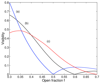
Figure 2: Talbot-Lau visibilities for ideal binary gratings as a function of the open fraction. (a) $L=L_{\lambda}$ (b) $L=0.9L_{\lambda}$ (c) $L=0.8L_{\lambda}$. The corresponding classical visibilities are all identical with curve (a).

As predicted by (32) the quantum and classical results are identical for $L/{L_{\lambda}}=1$ and given by Fig. 2(a). For $L/{L_{\lambda}}=0.9$ (Fig. 2(b)) and $L/{L_{\lambda}}=0.8$ (Fig. 2(c)) on the other hand, the Talbot-Lau visibilities differ markedly while the classical predictions remain on Fig. 2(a). The distinction between the classical and the quantum predictions is most pronounced for an opening fraction of $0.5$, where the classical contrast vanishes. The quantum calculation yields significant visibilities for these gratings, of $14.7\%$ at $L/{L_{\lambda}}=0.9$ and $25.4\%$ at $L/{L_{\lambda}}=0.8$, respectively.

II.4 Finite longitudinal coherence

In the above calculations the particle beam that enters the interferometer was assumed to have a fixed velocity in the $z$-direction and to be completely uncollimated in the transverse direction. Of course this is an idealization that is in many respects as unrealistic as the familiar assumption of a perfectly coherent plane wave. Realistic particle beams are characterized by a finite longitudinal coherence and show some correlations in the transverse direction.

The particle beams used in matter wave interferometry are usually generated by an effusive or supersonic expansion into a vacuum chamber Scoles et al. (1988). By means of additional skimmers or collimators the beam is restricted to a well-defined “longitudinal” direction. The beam is stationary, and as a consequence the longitudinal momenta show no off-diagonal elements in their density matrix Rubenstein et al. (1999). They are completely characterized by the longitudinal momentum distribution $g(p_{z})$ Englert et al. (1994).

The transverse momenta are much smaller than the longitudinal ones and can be taken to be uncorrelated with the longitudinal velocity. The transverse coherence is determined by the source aperture Born and Wolf (1980), and it could be calculated with the van Cittert-Zernike theorem Born and Wolf (1980) if the aperture size were small compared to the length scale in question. However, in the Talbot-Lau setup the source aperture is much larger than the spacing between the grating slits. As a consequence, diffraction at the first grating cannot be observed and it is permissible to approximate the transverse degrees of freedom as completely uncollimated. In front of the first grating the bulk of the beam is therefore appropriately characterized by the Wigner function,

$$W_{\mathrm{beam}}(\mathbf{R},\mathbf{P})=g(\mathbf{P}\cdot\mathbf{e}_{z}),$$ (33)

for $\mathbf{R}=\mathbf{r}+z\mathbf{e}_{z}$ with $z<0.$ This description does not account for the edges of the beam and the cut-off at larger transverse momenta, which is why it cannot be properly normalized. Fortunately, it is not necessary to include the full beam profile in the treatment of the Talbot-Lau effect. As shown below only the interference of paths through a few neighboring slits is relevant for the effect, so that the transverse variation of the total current can be neglected.

Formally, the beam (33) can be written as a convex sum of states $w(\mathbf{r},\mathbf{p})=1$ that are uniform in the transverse coordinates $\mathbf{r}$ and $\mathbf{p}$, and that have a fixed longitudinal momentum $p_{z}$.

$$W_{\mathrm{beam}}(\mathbf{r}+z\mathbf{e}_{z},\mathbf{p}+p_{z}\mathbf{e}_{z})=\int_{0}^{\infty}\delta(p_{z}-p_{z}^{\prime})\,\underbrace{w(\mathbf{r},\mathbf{p})}_{=1}\,g(p_{z}^{\prime})\,\mathrm{d}p_{z}^{\prime}.$$ (34)

Those are the states $w(\mathbf{r},\mathbf{p})=1$ that we started out with in Sect. II.2. Since a sequence of grating transmissions (9) and free evolutions (8) does not affect the dependence on $p_{z}$ the general stationary state at $z^{\prime}>0$ is given by

$$W_{\mathrm{beam}}(\mathbf{r}+z^{\prime}\mathbf{e}_{z},\mathbf{p}+p_{z}\mathbf{e}_{z})=w(z^{\prime};\mathbf{r},\mathbf{p})g\left(p_{z}\right)$$ (35)

and the transverse position density reads

$$w\left(\mathbf{r}\right) =\int\mathrm{d}\mathbf{p}\mathrm{d}p_{z}W_{\mathrm{beam}}(\mathbf{r}+z^{\prime}\mathbf{e}_{z},\mathbf{p}+p_{z}\mathbf{e}_{z})$$

$$=\int\mathrm{d}\mathbf{p}\mathrm{d}p_{z}~{}w(z^{\prime};\mathbf{r},\mathbf{p})g\left(p_{z}\right).$$ (36)

It follows that the finite longitudinal coherence in the beam is completely accounted for by averaging the results for a fixed velocity derived in Sects. II.2 and II.3 over the longitudinal velocity distribution. In particular, the modulation signals (22) and (30) are given by

$$\langle S(x_{\mathrm{s}})\rangle=\int_{0}^{\infty}\mathrm{d}p_{z}~{}g(p_{z})S(x_{\mathrm{s}}).$$ (37)

If the detection signal is proportional to the flux the average involves the longitudinal velocity component,

$$\langle S(x_{\mathrm{s}})\rangle=\frac{\int_{0}^{\infty}\mathrm{d}p_{z}~{}g(p_{z})p_{z}S(x_{\mathrm{s}})}{\int_{0}^{\infty}\mathrm{d}p_{z}~{}p_{z}g(p_{z})}.$$ (38)

Note that in either case the visibilities are not obtained by a simple average of (23) and (31), but have to be calculated from the averaged signal.

III The influence of realistic gratings

So far it has been assumed that the gratings are ideal in the sense that their thickness could be neglected. However, real gratings have a finite thickness and the time of interaction between the particle and the grating depends on the velocity $v_{z}=p_{z}/m_{\mathrm{p}}$ of the beam particles. This introduces a velocity dependence of the grating function both in the classical and in the quantum treatments. Generally speaking, the Talbot-Lau effect is affected more strongly by the grating forces than far-field diffraction Brühl et al. (2002a), since the near-field interference is characterized by smaller phase shifts. This was seen in recent experiments with beams of large molecules Brezger et al. (2002); Hornberger et al. (2003); Hackermüller et al. (2003a, 2004).

III.1 The grating interaction

In order to account for the effect of a finite grating thickness $b$ we consider an additional interaction potential $V(x)$ that acts while the particle is traversing the grating. In order to avoid a more detailed $z$-dependence in the potential we average over the the surface roughness and assume that the grating walls are parallel to the optical axis and that edge effects can be neglected. In the case of tilted walls one can introduce an effective slit width, as discussed in Stoll (2003). Moreover, it is known Grisenti et al. (1999); Brühl et al. (2002b) that grating interaction effects are usually well described by the eikonal approximation. There, the additional quantum phase due to the interaction potential $V(x)$ is obtained by integrating the action along a straight path. Accordingly, if we take the binary function $t(x)$ to describe the material grating the complete grating function is given by

$$\tilde{t}(x)=t(x)\exp\!\left(-\mathrm{i}\frac{m_{\mathrm{p}}b}{p_{z}}\frac{V(x)}{\hbar}\right).$$ (39)

Here and below the tilde is used to indicate quantities which have an additional velocity dependence due to the grating interaction. Accordingly, for non-ideal gratings the convolution kernel (10) is replaced by

$$\widetilde{T}(x,p)=\int\mathrm{d}q\,T(x,p-q)T_{V}(x,q)$$ (40)

with

$$T_{V}(x,q)=\frac{1}{2\pi\hbar}\int\mathrm{d}\Delta\,\mathrm{e}^{\mathrm{i}q\Delta/\hbar}\\ \times\exp\!\left(-\mathrm{i}\frac{m_{\mathrm{p}}b}{p_{z}\hbar}\left[V\left(x-\frac{\Delta}{2}\right)-V\left(x+\frac{\Delta}{2}\right)\right]\right)\;.$$ (41)

It follows that the quantum expressions (19) for the density pattern and (23) for the signal visibility still hold after the replacement

$$B_{m}^{(\lambda)}\rightarrow\widetilde{B}_{m}^{(\lambda)}=\sum_{j\in\mathbb{Z}}\tilde{b}_{j}\tilde{b}_{j-m}^{\ast}\exp\!\left(\mathrm{i}\pi\frac{m^{2}-2jm}{2}\frac{L}{{L_{\lambda}}}\right)$$ (42)

with the modified Fourier components $\tilde{b}_{m}=\sum b_{j}\tilde{c}_{m-j}$ and

$$\tilde{c}_{m}=\frac{1}{d}\int_{-\frac{d}{2}}^{\frac{d}{2}}\mathrm{e}^{-2\pi\mathrm{i}m{x}/{d}}\exp\!\left(-\mathrm{i}\frac{m_{\mathrm{p}}b}{p_{z}}\frac{V(x)}{\hbar}\right)\mathrm{d}x\;.$$ (43)

As mentioned above the presence of $V(x)$ introduces a velocity dependence also on the classical level. This can be seen by considering the local approximation of (41) where terms of the order $\partial_{x}^{3}V(x)\Delta^{3}$ are neglected in the exponent,

$$T_{V}(x,q) \simeq\,\frac{1}{2\pi\hbar}\int\mathrm{d}\Delta\,\exp\!\left(\mathrm{i}\left[q+\frac{m_{\mathrm{p}}b}{p_{z}}\frac{\mathrm{d}}{\mathrm{d}x}V(x)\right]\frac{\Delta}{\hbar}\right)$$

$$=\delta\left(q+\frac{m_{\mathrm{p}}b}{p_{z}}\frac{\mathrm{d}}{\mathrm{d}x}V(x)\right).$$ (44)

According to (40) this yields a classical convolution kernel

$$\widetilde{T}_{\mathrm{cl}}(x,p) =|t_{2}(x)|^{2}\delta\left(p+\frac{m_{\mathrm{p}}b}{p_{z}}\frac{\mathrm{d}}{\mathrm{d}x}V(x)\right)$$

$$\equiv|t_{2}(x)|^{2}\delta(p-Q(x))$$ (45)

which indicates that the eikonal approximation corresponds on the classical level to the momentum kick $Q(x)=-\partial_{x}V(x)\times b/v_{z}$ obtained by multiplying the constant classical force at a fixed position $x$ with the interaction time. Accordingly, the classical phase space distribution changes as $f^{\prime}(x,p)=|t(x)|^{2}f(x,p-Q(x))$ when passing a grating. Using this transformation and the periodicity of $Q$ one finds that the classical expressions for the density pattern and for the signal visibility assume the forms (28) and (31) as in the ideal case. One merely has to replace the Fourier components by

$${B}_{n}^{(0)}\rightarrow\widetilde{B}_{n}^{(0)}=\sum_{m\in\mathbb{Z}}{B}_{m}^{(0)}\widetilde{C}_{n-m}^{n}$$ (46)

with

$$\widetilde{C}_{m}^{n}=\frac{1}{d}\int_{-\frac{d}{2}}^{\frac{d}{2}}\mathrm{e}^{-2\pi\mathrm{i}m{x}/{d}}\exp\left(-\mathrm{i}\pi n\frac{L}{d}\frac{Q(x)}{p_{z}}\right)\mathrm{d}x\;.$$ (47)

We note that the modifications of the Fourier components given by (42) and (46) describe the quantum and the classical interactions on the same degree of approximation. Clearly, the fact that the interaction with the grating is treated equally in the quantum and in the classical descriptions is an important requirement for identifying quantum interference in an experimental observation.

Before turning to realistic descriptions for the grating interaction we note that it is in general not necessary to include the grating interaction at the first and third gratings. This is clear from the fact that the Talbot-Lau setup is sensitive to diffraction only at the second grating, while the others merely serve to modulate the flux. Formally, it can be seen from the expression for the observed signal, Equation (21) with (13). It depends only on the squared moduli $|t_{1}(x)|^{2}$ and $|t_{3}(x)|^{2}$ of the first and third grating function, which are not affected by the phase shift in (39). Only for very strong potentials, where (39) is no longer valid, may the interaction effectively reduce the slit width and thus become relevant to the first and third grating.

III.2 Material gratings

A neutral particle will in general experience an attractive van der Waals force if placed in the vicinity of a surface. A simple, but quite realistic description for nonpolar quantum objects is given by the static London dispersion force which acts between a quantum object and a flat wall. If $\Delta$ is the distance to the wall it gives rise to the potential $U(\Delta)=-C_{3}/\Delta^{3}$, with $C_{3}>0$ Dzyaloshinskii et al. (1961).

For simple wall materials the interaction constant $C_{3}$ can be found in the literature for many atoms and a number of small molecules Vidali et al. (1991). In general it is obtained from the Lifshitz formula Dzyaloshinskii et al. (1961); McLachlan (1964); Zaremba and Kohn (1976)

$$C_{3}=\frac{\hbar}{4\pi}\int_{0}^{\infty}\alpha(\mathrm{i}\omega)\frac{\epsilon(\mathrm{i}\omega)-1}{\epsilon(\mathrm{i}\omega)+1}\mathrm{d}\omega\,$$ (48)

by using either experimental data (e.g. absorption spectra) or appropriate models for the dynamic polarizability $\alpha$ of the particle and for the bulk dielectric function $\epsilon$ of the grating material, respectively. Often Drude-type models for $\alpha$ and $\epsilon$ are considered sufficient. In Grisenti et al. (1999); Brühl et al. (2002b) the interaction with material gratings was studied in an interference experiment and found to be in good agreement with the assumption of a London dispersion force.

However, at large distances retardation effects may become important. They show up if the separation $\Delta$ between the particle and the grating wall is comparable to the wavelength corresponding to those virtual transitions in the particle that contribute with a large oscillator strength. In the case of an ideal metal the potential is described by the Casimir-Polder formula Casimir and Polder (1948). For large distances it has the asymptotic form $U(\Delta)=-C_{4}/\Delta^{4}$ with the constant

$$C_{4}=\frac{3\hbar c}{8\pi}\,\alpha(0)$$ (49)

given by the static polarizability $\alpha(0)$ of the particle. The case of more realistic grating materials and arbitrary distances is covered by the theory of Wylie and Sipe Wylie and Sipe (1984, 1985). It shows that in the case of real metals the asymptotic form of the interaction potential does not depend on the metal and is identical to the ideal case. For dielectrics the limiting form depends also on the fourth power of the distance, but with a reduced interaction constant,

$$C_{4}^{\epsilon}=C_{4}\,\int_{0}^{\infty}\frac{(1+2u^{2})r_{\mathrm{p}}(u)-r_{\mathrm{s}}(u)}{(1+u^{2})^{5/2}}\,\frac{u}{2}\,\mathrm{d}u.$$ (50)

The reduction depends on the static dielectric constant $\epsilon(0)$ via the Fresnel coefficients

$$r_{\mathrm{p}}(u)=\frac{\sqrt{1+u^{2}}-\sqrt{\epsilon(0)+u^{2}}}{\sqrt{1+u^{2}}+\sqrt{\epsilon(0)+u^{2}}}$$ (51)

and

$$r_{\mathrm{s}}(u)=\frac{\epsilon(0)\sqrt{1+u^{2}}-\sqrt{\epsilon(0)+u^{2}}}{\epsilon(0)\sqrt{1+u^{2}}+\sqrt{\epsilon(0)+u^{2}}}\;.$$ (52)

Figure 3 gives the value of the dielectric reduction factor for $1\leq\epsilon(0)\leq 100$.

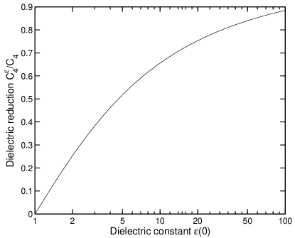
Figure 3: Reduction factor $C_{4}^{\varepsilon}/C_{4}$, see Eq. (50), of the long-range interaction for dielectric gratings as compared to ideal metals (semi-logarithmic scale). For typical grating materials the static dielectric constant $\varepsilon\left(0\right)$ is less than 4, leading to a reduction below one half.

Whether the exact position dependence of the retarded force must be used depends on the physical situation in the particular interferometric setup. In most experiments realized so far it was sufficient to use either the static van der Waals interaction (48) Brühl et al. (2002a)or the long range limit of the Casimir-Polder force, Equation (49).

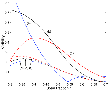
Figure 4: Talbot-Lau visibilities for gratings with a van der Waals interaction as a function of the open fraction. (a) $L=L_{\lambda}$ (b) $L=0.9L_{\lambda}$ (c) $L=0.8L_{\lambda}$. The corresponding classical visibilities are given by the curves (d), (e), (f), respectively.

Figure 4 shows the typical effect of a finite grating interaction, and should be compared to the results for the ideal grating in Fig. 2. Here we assume a particle with mass $1000\,\mathrm{amu}$, a van der Waals interaction with $C_{3}=10\,\mathrm{meV\,nm^{6},}$ and we take gratings with a period of $d=1\,\mathrm{\mu m}$ and a thickness of $b=0.2\,\mathrm{\mu m}$ separated by a distance of $L=0.2\,$m. One observes that the expected quantum visibilities deviate noticeably from the ideal case. Moreover, the classical expectations (given by the dashed lines) differ completely from the ideal expectation and display now a weak velocity dependence. At an open fraction of $0.5$ they now yield a finite contrast amounting to $12.4\%-12.9\%$ for the three settings. The respective quantum expectations are also larger than the in the force-free calculation. (They increased from 14.7% to 32.9% at $L/{L_{\lambda}}=0.9$ and from 25.4% to 35% at $L/{L_{\lambda}}=0.8$.) This is a typical phenomenon. The attractive force tends to act as if the open fraction of the grating was decreased.

III.3 Gratings of light

It is clear from Equations (13) and (21) that the first and the third gratings in the Talbot-Lau setup must be absorptive to generate an observable contrast pattern. However, as discussed in Brezger et al. (2003) the second grating may be a pure phase grating as well. Such a mixed interferometer can be realized by the off-resonant interaction with a standing light wave Kapitza and Dirac (1933), see Nairz et al. (2001) for the laser diffraction of large molecules.

If we take a TEM₀₀ mode of wavelength $\lambda_{\mathrm{L}}=2\pi/k_{\mathrm{L}}$ and waist $w$ produced by a laser of power $P_{\text{L}}$ then the dipole force leads to the phase shift

$$\tilde{t}(x)=\exp\left(\mathrm{i}\sqrt{2\pi}\frac{8P_{\text{L}}\alpha_{\omega}}{\hbar cv_{z}w}\cos^{2}(k_{\mathrm{L}}x)\right),$$ (53)

as follows from an integration over the gaussian beam at central passage. Here $\alpha_{\omega}$ is the scalar polarizability [73] of the particle at Laser frequency $\omega_{\mathrm{L}}=ck_{\mathrm{L}}$, where we assume that $\operatorname{Im}(\alpha_{\omega})=0$ so that photon absorption can be neglected. The classical momentum kick in (45) that corresponds to the dipole force reads

$$Q(x)=\sqrt{2\pi}\frac{8P_{\text{L}}\alpha_{\omega}\,k_{\mathrm{L}}}{cv_{z}w}\sin(2k_{\mathrm{L}}x)\;.$$ (54)

Using these expressions in (39) and (47) one obtains the predictions for the quantum and classical density patterns produced by a standing light wave in the same way as with material gratings.

In the present section we showed that the Wigner description of the Talbot-Lau effect permits the effects of the grating interaction to be incorporated easily, in terms of a simple modification of the Fourier coefficients. As discussed in the next section the effect of decoherence can be similarly incorporated into the formalism.

IV Accounting for decoherence

Having formulated the Talbot-Lau dynamics in the Wigner representation it is now easy to include the effects of decoherence. More specifically, we consider the markovian interaction of the interfering particle with other, unobserved degrees of freedom (the environment) Joos et al. (2003); Zurek (2003). The resulting formation of quantum correlations (or entanglement) between the particle and the environment leads to a loss of coherence in the particle state that may be understood from the fact that a measurement of the environmental degree of freedom could reveal (partial) which-way information on the particle’s whereabouts.

We note that a number of studies have been undertaken recently that describe a loss of visibility in matter wave interference Bonifacio and Olivares (2002); Facchi et al. (2002); Viale et al. (2003). Here we focus on the Talbot-Lau effect and on a formulation that is sufficiently realistic to permit quantitative predictions about experiments with mesoscopic bodies Hornberger et al. (2003); Hackermüller et al. (2004).

Two important decoherence mechanisms for large, interfering particles are collisions with background gas particles and the thermal emission of electromagnetic radiation. Both effects may be treated in the Markov approximation, which implies that the effect of the environmental coupling can be described by independent, separate events (such as the emission of a photon or the collision with a gas particle).

IV.1 The effect of a single decoherence event

The change in the state of the interfering particle due to a single event can be obtained by performing a partial trace over the entangled state with respect to the unobserved degrees of freedom. For particles with a large mass and for the decoherence mechanisms considered in this article the density matrix in position representation changes just by a multiplication,

$$\varrho^{\prime}(\mathbf{R}_{1},\mathbf{R}_{2})=\varrho(\mathbf{R}_{1},\mathbf{R}_{2})\,\eta(\mathbf{R}_{1}-\mathbf{R}_{2}).$$ (55)

The factor $\eta(\mathbf{R}_{1}-\mathbf{R}_{2}),$ which may be called the decoherence function, describes the decay of the off-diagonal elements (the coherences) of $\hat{\varrho}$ due to a single event. In Sect. V we will derive the form of realistic decoherence functions for the most important decoherence mechanisms. For the time being it is sufficient to note that the conservation of the trace in (55) ensures that

$$\lim_{\mathbf{\mathbf{R}_{1}\rightarrow\mathbf{R}_{2}}}\eta(\mathbf{R}_{1}-\mathbf{R}_{2})=1,$$ (56)

so that the diagonal elements of the state are unchanged by (55). Moreover, the hermiticity of $\hat{\varrho}$ implies $\eta\left(-\mathbf{R}\right)=\eta^{\ast}\left(\mathbf{R}\right),$ and from the fact that the purity cannot be increased by a partial trace it follows that $|\eta(\mathbf{R}_{1}-\mathbf{R}_{2})|\leq 1.$

If the state is expressed in terms of the Wigner function its change (55) reads

$$W^{\prime}(\mathbf{R},\mathbf{P})=\int\mathrm{d}\mathbf{Q}\,\bar{\eta}(\mathbf{Q})W(\mathbf{R},\mathbf{P}-\mathbf{Q}).$$ (57)

with $\bar{\eta}(\mathbf{Q})$ the Fourier transform of the decoherence function,

$$\bar{\eta}(\mathbf{Q})=\frac{1}{\left(2\pi\hbar\right)^{3}}\int\mathrm{d}\mathbf{R~{}}e^{-\mathrm{i}\mathbf{QR/\hbar}}\eta\left(\mathbf{R}\right).$$ (58)

Clearly, the effect of a decoherence event on the Wigner function is to smear it out in the momentum direction.

As discussed in Sect. II.4 the coherently evolving, stationary state of the beam in a Talbot-Lau interferometer is described by the function

$$W_{\mathrm{beam}}(\mathbf{r}+z\mathbf{e}_{z},\mathbf{p}+p_{z}\mathbf{e}_{z})=w(z;\mathbf{r},\mathbf{p})g(p_{z}).$$ (59)

In a typical setup the grating constant and the grating separation differ by six orders of magnitude so that $\mathbf{p}$ varies on a scale in (59) that is much smaller than the magnitude of $p_{z}.$ Our basic approximation is now to assume that the width of $\bar{\eta}$ is small compared to the scale over which $W_{\mathrm{beam}}$ varies in $p_{z}$. This assumption is particularly unproblematic in the Talbot-Lau setup, where the sensitivity to changes in the longitudinal momentum is rather weak. It follows that the new state of the transverse coordinates is approximately given by integrating the full state with respect to the longitudinal momentum,

$$w^{\prime}(z;\mathbf{r},\mathbf{p})\simeq\int\mathrm{d}p_{z}^{\prime}\mathbf{~{}}W_{\text{beam}}^{\prime}\left(\mathbf{r}+z\mathbf{e}_{z},\mathbf{p}+p_{z}^{\prime}\mathbf{e}_{z}\right).$$ (60)

Inserting (57) and (59) yields the change in the state of the transverse coordinates

$$w^{\prime}(z;\mathbf{r},\mathbf{p})=\int\mathrm{d}\mathbf{q~{}}\bar{\eta}_{\mathrm{2d}}(\mathbf{q)~{}}w\left(z;\mathbf{r},\mathbf{p}-\mathbf{q}\right)$$ (61)

with

$$\bar{\eta}_{\mathrm{2d}}(\mathbf{q)}\equiv\int\mathrm{d}q_{z}~{}\bar{\eta}(\mathbf{q}+q_{z}\mathbf{e}_{z}).$$ (62)

It follows from (62) that in the position representation of the transverse state, $\rho(\mathbf{r}_{1},\mathbf{r}_{2}),$ the decoherence function enters without modification,

$$\rho^{\prime}(\mathbf{r}_{1},\mathbf{r}_{2}) =\rho(\mathbf{r}_{1},\mathbf{r}_{2})\,\int\mathrm{d}\mathbf{q~{}}\mathrm{e}^{\mathrm{i}\mathbf{q}\left(\mathbf{r}_{1}-\mathbf{r}_{2}\right)/\hbar}\bar{\eta}_{\mathrm{2d}}(\mathbf{q)}$$

$$=\rho(\mathbf{r}_{1},\mathbf{r}_{2})\,\eta\left(\mathbf{r}_{1}-\mathbf{r}_{2}\right),$$ (63)

but restricted to the $xy$-plane, $\eta\left(\mathbf{r}\right)\equiv\eta\left(\mathbf{r}+0\mathbf{e}_{z}\right).$

Using the Wigner function it is now possible to evaluate the effect of a single decoherence event that takes place at a distance $z$ behind the first grating. One merely propagates the state to the longitudinal position $z$ using the coherent transformations (8) and (9), then applies (61), and propagates the state over the remaining distance to the third grating. Within the paraxial approximation no additional error is introduced by this procedure since the composition property of the evolution holds exactly. The result takes a simple form (both for $z<L$ and for $z>L$) once the momentum is integrated to yield the position density $w\left(\mathbf{r}\right)$ in front of the third grating. It is given by an integral of the form (13),

$$w\left(\mathbf{r}\right)=\int\mathrm{d}\mathbf{r}_{1}|t_{1}\left(\mathbf{r}_{1}\right)|^{2}\hat{h}_{z}(\mathbf{r};\mathbf{r}_{1}),$$ (64)

where the coherent kernel $h\left(\mathbf{r},\mathbf{r}_{1}\right)$ from (14) is replaced by

$$\hat{h}_{z}(\mathbf{r};\mathbf{r}_{1})=\int\mathrm{d}\mathbf{q}\,\bar{\eta}_{\mathrm{2d}}(\mathbf{q})~{}h\left(\mathbf{r},\mathbf{r}_{1}-\frac{L-|z-L|}{p_{z}}\mathbf{q}\right).$$ (65)

This shows clearly that close to the first and to the third grating, at $z=0$ and $z=2L$, a decoherence event will not affect the interference pattern while, for monotonically decreasing $\bar{\eta}_{\mathrm{2d}}(\mathbf{q}),$ the interference is most strongly affected by decoherence events that take place in the vicinity of the second grating, at $z=L$. This is consistent with the notion that in the Talbot-Lau setup diffraction takes place only at the second grating, while the first grating acts as an array of coherence slits.

We take the grating function again to be periodic in $x$ (with period $d)$ and uniform in $y.$ This means that the discussion can be confined to the $x$-coordinate like in Sect. II.2. Using the Fourier decomposition (16) one finds that the coherent kernel (14) reads in the one-dimensional case

$$h\left(x;x_{1}\right) \equiv\int\mathrm{d}y\mathrm{d}y_{1}h\left(x\mathbf{e}_{x}+y\mathbf{e}_{y};x_{1}\mathbf{e}_{x}+y_{1}\mathbf{e}_{y}\right)$$ (66)

$$=\frac{p_{z}}{2L\hbar}\sum_{m}\mathrm{\exp}\left(2\pi\mathrm{i}m\frac{x+x_{1}}{2d}\right)\tilde{B}_{m}^{(\lambda)}.$$

It follows with (65) that in the presence of a decoherence event the kernel takes the form

$$\hat{h}_{z}\left(x;x_{1}\right)= \frac{p_{z}}{2L\hbar}\sum_{m}\mathrm{\exp}\left(2\pi\mathrm{i}m\frac{x+x_{1}}{2d}\right)$$

$$\times\tilde{B}_{m}^{(\lambda)}\eta\left(-m\frac{d}{2}\frac{L-|z-L|}{{L_{\lambda}}}\mathbf{e}_{x}\right),$$ (67)

where the three dimensional decoherence function from (55) enters with its dependence along the $x$-axis. The comparison with (66) shows that the modified interference pattern corresponding to a single decoherence event at position $z$ is completely described by a modification of the coherent Fourier components (42)

$$\widetilde{B}_{m}^{(\lambda)}\rightarrow\widetilde{B}_{m}^{(\lambda)}\,\eta\left(-m\frac{d}{2}\frac{L-|z-L|}{{L_{\lambda}}}\mathbf{e}_{x}\right).$$ (68)

IV.2 An alternative to the master equation

One can now account for probabalistically occurring decoherence events by considering the change in the final interference pattern due to events that occur with rate $R(z)$ in the interval $(z;z+\mathrm{d}z)$. It follows from (68) that the corresponding Fourier coefficients satisfy the differential equation

$$\frac{\mathrm{d}}{\mathrm{d}z}\widehat{B}_{m}^{(\lambda)}=R(z)\left[\widehat{B}_{m}^{(\lambda)}\,\eta\left(-m\frac{d}{2}\frac{L-|z-L|}{{L_{\lambda}}}\mathbf{e}_{x}\right)-\widehat{B}_{m}^{(\lambda)}\right].$$ (69)

It describes the change of the interference pattern with an increasing size of the interval where decoherence events may occur. The integration of (69) over the whole range $z\in\left(0;2L\right)$ of admitted decoherence then yields the coefficients characterizing the modified pattern. They are given by

$$\widehat{B}_{m}^{(\lambda)}=\widetilde{B}_{m}^{(\lambda)}\exp\left(-\int_{0}^{2L}R(z)\left[1-\eta\left(-m\frac{d}{2}\frac{L-|z-L|}{{L_{\lambda}}}\mathbf{e}_{x}\right)\right]\mathrm{d}z\right),$$ (70)

with $\widetilde{B}_{m}^{(\lambda)}$ the coefficients of the coherent evolution. This is the central result of this section. It shows that the effects of markovian decoherence of the form (55) can be calculated analytically if the setup is insensitive to longitudinal correlations as in the Talbot-Lau interferometer. It follows immediately that the position density and the visibility of the modulation signal are given by the formulas (19) and (23), respectively, if the coherent coefficients $\widetilde{B}_{m}^{(\lambda)}$ are replaced by those of the incoherent evolution (70).

The result (70) can be easily generalized to the asymmetric Talbot-Lau interferometer. The case of several independent decoherence mechanisms is also easily incorporated. The resulting interference pattern is then characterized by a product of the corresponding exponentials in (70).

It is important to note that the basic Fourier components $m=0$ are not affected by decoherence, since $\eta\left(0\right)=1.$ This shows that the mean count rate does not change due to the presence of decoherence, as is to be expected from the conservation of the norm in (55). The reduction of the observed visibility assumes a compact form if the modulation signal (22) is (approximately) sinusoidal, as is typically the case for gratings with an open fraction of $f\simeq 0.5$. Then only the coefficients $\widehat{B}_{0}^{(\lambda)}$and $\widehat{B}_{2}^{(\lambda)}$contribute to the visibility if the grating periods are equal, $r=2$. With $\eta\left(0\right)=1$ it follows that the reduced visibility is given by

$$\mathcal{V}=\mathcal{V}_{0}\exp\left(-\int_{0}^{2L}R(z)\left[1-\eta\left(-d\frac{L-|z-L|}{{L_{\lambda}}}\mathbf{e}_{x}\right)\right]\mathrm{d}z\right),$$ (71)

where $\mathcal{V}_{0}$ indicates the visibility in the absence of decoherence. This formula is particularly intuitive if the Talbot criterion is met, $L=L_{\lambda}$. Then the argument of $\eta$ contains the separation of two paths that start and end at common points and pass the second grating through neighboring slits. At $z=L$ it is equal to the grating constant $d,$ which shows that the Talbot-Lau interference with equal gratings is based on the interference through neighboring slits. Also at other positions $z$ a reduced magnitude of $\eta$ suppresses the visibility whenever the change in the environmental state is able to resolve the corresponding path separation. Higher orders of the Talbot effect, $L=mL_{\lambda}$ with $m\in\mathbb{N}$, correspond to multiple slit separations $md$. For longitudinal velocities that deviate from the Talbot criterion with $L\neq mL_{\lambda}$ the argument is replaced by an “effective” path separation.

It should be emphasized that our derivation of (70) and (71) is rather different from solving the markovian master equation corresponding to the decoherence mechanism. In Sect. VI we obtain a solution of the master equation corresponding to decoherence of the type (55) for a general interfering state in the paraxial approximation. An expression analogous to (71) is found there, albeit in a time-dependent formulation, see (120). This vindicates our approximation (60).

The present formulation has the particular advantage that the rate $R$ of decoherence events and their effect $\eta$ appear separately in the equation. This might seem to be a complication, since these two quantities must be calculated independently by quantum mechanical means. However, they are often needed with different degrees of sophistication. For example, often one must take into account the position dependence of the rate. This is easily incorporated in the present framework, while solving a corresponding master equation would be incomparably more complicated.

IV.3 Quantum decoherence vs. a classical stochastic process

Having treated the effect of environmental coupling on the quantum evolution, we can now turn to its effects in the classical description. In Sect. II.3 the classical expectation was calculated in terms of the phase space density $f(\mathbf{r},\mathbf{p}).\$The close analogy between the quantum problem and the classical calculation allows to map the Wigner representation of a decoherence event (61) to the classical description. It follows from (61) that the effect of a decoherence event can be interpreted on the classical level as a probabilistic momentum kick,

$$f^{\prime}(\mathbf{r},\mathbf{p})=\int\mathrm{d}\mathbf{q~{}}\bar{\eta}_{\mathrm{2d}}(\mathbf{q)~{}}f\left(\mathbf{r},\mathbf{p}-\mathbf{q}\right).$$ (72)

Indeed, the properties $\eta\left(0\right)=1$ and $\eta\left(-\mathbf{r}\right)=\eta^{\ast}\left(\mathbf{r}\right)$ of the decoherence function imply that $\bar{\eta}_{\mathrm{2d}}$ has the features of a probability density, $\bar{\eta}_{\mathrm{2d}}(\mathbf{q)}\geq 0$ and $\int\mathrm{d}\mathbf{q~{}}\bar{\eta}_{\mathrm{2d}}\left(\mathbf{q}\right)=1.$ From the close analogy of the classical and the quantum expressions for the free evolution and the passage through a grating it is easy to see that the above derivation of the modified pattern holds in the classical formulation as well if one replaces the quantum coefficients $\widetilde{B}_{m}^{(\lambda)}$ in (70) by their classical counterparts $\widetilde{B}_{m}^{(0)}$.

From this one might be led to conclude that the decoherence described in (55) was a “classical effect”. In our view this would be a misinterpretation, since a probabilistic formulation is possible only if the Wigner function is non-negative everywhere, that is, if it cannot be distinguished from a classical probability distribution. If the Wigner function is negative in some parts, as is the case for an interfering state, any stochastic interpretation is invalidated by the occurring flux of a “negative probability”. Notwithstanding this, once the motional state has turned into a classical state without negativities in the Wigner function the additional loss of visibility in the quantum description is indeed indistinguishable from a corresponding classical stochastic process.

V Realistic decoherence functions

In the following we discuss the form of realistic decoherence functions that can be used to obtain quantitative predictions on the effects of decoherence in matter wave experiments. We focus on the most important mechanisms for large, massive objects, namely, collisions with particles from the background gas and the emission of heat radiation. We note that simple estimates of these effects on material particles can be found in Joos and Zeh (1985); Tegmark (1993); Alicki (2002).

V.1 Decoherence by collisions with gas particles

A very important source of decoherence is the unavoidable presence of a background gas in the experimental apparatus. Typically, the mass of the interfering particles is much larger than the mass of the gas particles, $m_{\mathrm{p}}\gg m_{\mathrm{g}},$ and the interaction is of the monopole type. In this case the decoherence function reads Joos and Zeh (1985); Gallis and Fleming (1990); Hornberger and Sipe (2003)

$$\eta(\mathbf{R}_{1},\mathbf{R}_{2})=\operatorname{tr}_{\text{gas}}\left\{\mathrm{\exp}\left(-\mathrm{i}\mathbf{\hat{P}}_{\text{gas}}\frac{\mathbf{R}_{2}}{\hbar}\right)\hat{S}_{0}^{{\dagger}}~{}\mathrm{\exp}\left(\mathrm{i}\mathbf{\hat{P}}_{\text{gas}}\frac{\mathbf{R}_{2}-\mathbf{R}_{1}}{\hbar}\right)\hat{S}_{0}~{}\mathrm{\exp}\left(-\mathrm{i}\mathbf{\hat{P}}_{\text{gas}}\frac{\mathbf{R}_{1}}{\hbar}\right)\hat{\varrho}_{\text{gas}}\right\}\;$$ (73)

where $\mathbf{\hat{P}}_{\text{gas}}$ is the momentum operator of the gas particles and $\hat{S}_{0}$ the center-of-mass scattering operator. The trace over the scattered gas particle in (73) can be evaluated if it is in a (thermal) state that is diagonal in momentum and characterized by the distribution $\mu_{\text{gas}}\left(\mathbf{P}\right).$ One obtains Gallis and Fleming (1990); Hornberger and Sipe (2003)

$$\eta(\mathbf{R}_{1},\mathbf{R}_{2})=\int\mathrm{d}\mathbf{P}~{}\mu_{\text{gas}}\left(\mathbf{P}\right)\bigg{[}1-\int\mathrm{d}\mathbf{P}^{\prime}~{}\left(1-\mathrm{e}^{\mathrm{i}\left(\mathbf{P}-\mathbf{P}^{\prime}\right)\left(\mathbf{R}_{1}-\mathbf{R}_{2}\right)/\hbar}\right)\underset{X_{\Omega}}{\underbrace{\frac{\left(2\pi\hbar\right)^{3}}{\Omega}|\langle\mathbf{P}^{\prime}|\mathcal{\hat{T}}_{0}|\mathbf{P}\rangle|^{2}}}~{}\bigg{]}$$ (74)

with $\hat{T}_{0}=\mathrm{i}(1-\hat{S}_{0}).$ Awkwardly, the last two expressions in (74), which are indicated by $X_{\Omega}$, involve two quantities that are arbitrarily large. One is the “quantization volume” $\Omega$, which originates from the normalization of the thermal state $\hat{\varrho}_{\text{gas}},$ and the other is the square of the delta function appearing in the matrix element $\langle\mathbf{P}^{\prime}|\hat{T}_{0}|\mathbf{P}\rangle=f(\mathbf{P}^{\prime},\mathbf{P})\delta\left(P^{\prime}-P\right)/(2\pi\hbar P).$ Here $f(\mathbf{P}^{\prime},\mathbf{P})$ is the scattering amplitude (which must not be confused with the classical phase space density from Sect. II.3). Since the decoherence function is well defined by Equation (73) these two infinite quantities must cancel if the limit $\Omega\rightarrow\infty$ is taken properly. As argued in Hornberger and Sipe (2003) physical consistency requirements lead to

$$\lim_{\Omega\rightarrow\infty}X_{\Omega}=\frac{|f(\mathbf{P}^{\prime},\mathbf{P})|^{2}}{\sigma\left(P\right)}\frac{\delta\left(P^{\prime}-P\right)}{P^{2}}$$ (75)

where $\sigma\left(P\right)$ is the total scattering cross section

$$\sigma\left(P\right)=\int\!\!\mathrm{d}\mathbf{n~{}}|f(P\mathbf{n},\mathbf{P})|^{2}.$$ (76)

With the replacement (75) one gets

$$\eta(\mathbf{R}_{1},\mathbf{R}_{2}) =\int\!\!\!\mathrm{d}\mathbf{P}~{}\frac{\mu_{\text{gas}}\left(\mathbf{P}\right)}{\sigma(P)}$$ (77)

$$\times\int\!\!\mathrm{d}\mathbf{n}~{}\left|f\left(\cos(\theta)\right)\right|^{2}\,\mathrm{e}^{\mathrm{i}\left(\mathbf{P}-P\mathbf{n}\right)\left(\mathbf{R}_{1}-\mathbf{R}_{2}\right)/\hbar}.$$

As already anticipated in Equation (55) this function depends only on the position difference $\mathbf{R}_{1}-\mathbf{R}_{2}.$ For an isotropic distribution of the gas momenta, $\mu_{\text{gas}}\left(\mathbf{P}\right)=\nu_{\text{gas}}\left(P\right)/\left(4\pi P^{2}\right),$ the expression can be further simplified noting that it depends only on the distance $\Delta R=|\mathbf{R}_{1}-\mathbf{R}_{2}|.$ One obtains

$$\eta(\Delta R) =\int_{0}^{\infty}\!\!\!\mathrm{d}P\;\frac{\nu_{\text{gas}}(P)}{\sigma(P)}$$ (78)

$$\times\int\!\!\mathrm{d}\Omega~{}\left|f\left(\cos(\theta)\right)\right|^{2}\,{\mathrm{sinc}}\!\left({\sin\!\left(\frac{\theta}{2}\right)}\frac{2P\Delta R}{\hbar}\right)$$

with $\operatorname{sinc}\left(x\right)=\sin\left(x\right)/x.$ The argument of the $\operatorname{sinc}$ function is equal to the momentum transfer during the collision times the distance $\Delta R$ in units of $\hbar.$ This indicates that whenever the change in the state of the gas particle suffices to resolve the distance $\Delta R$ the corresponding coherences in the motional state will be suppressed.

Let us turn to the second ingredient to the decoherence formula (71), the scattering rate $R(z).$ It is usually expressed in terms of an effective cross section, $R\left(z\right)=n\left(z\right)\sigma_{\mathrm{eff}},$ with $n\left(z\right)$ the number density of the background gas. For a constant density, and again $m_{\mathrm{p}}\gg m_{\mathrm{g}},$ the effective cross section depends only on the velocity of the interfering particle. It is given by

$$\sigma_{\mathrm{eff}}\left(v_{\mathrm{p}}\right)=\int\mathrm{d}\mathbf{P}~{}\mu_{\text{gas}}\left(\mathbf{P}\right)\sigma\left(|\mathbf{P}-m_{\mathrm{g}}v_{\mathrm{p}}\mathbf{e}_{\mathrm{z}}|\right)\frac{|\mathbf{P/}m_{\mathrm{g}}-v_{\mathrm{p}}\mathbf{e}_{\mathrm{z}}|}{v_{\mathrm{p}}},$$ (79)

as follows from the derivation of the Boltzmann equation.

The most prominent interaction encountered in molecular scattering is the van der Waals force between polarizable molecules. At the typical velocities in matter wave interferometry the scattering depends only on the long-range part of the interaction potential, $U\left(r\right)=-C_{6}/r^{6}$, which is characterized by a single interaction constant $C_{6}.$ The total cross section is then independent of mass and given by Maitland et al. (1981)

$$\sigma\left(m_{\mathrm{g}}v\right)=\frac{\pi^{2}}{\Gamma\left(2/5\right)\sin\left(\pi/5\right)}\left(\frac{3\pi}{8}\frac{C_{6}}{\hbar v}\right)^{2/5}.$$ (80)

The integration in (79) can be done assuming a thermal distribution of the gas particles. The exact expression is given by a confluent hypergeometric function, as shown recently by Vacchini Vacchini (2004). Here we note the asymptotic form of the effective cross section (79) for small velocities of the interfering particle. It reads

$$\sigma_{\mathrm{eff}}\left(v_{\mathrm{p}}\right) =\frac{4\pi\Gamma\left(9/10\right)}{5\sin\left(\pi/5\right)}\left(\frac{3\pi C_{6}}{2\hbar}\right)^{2/5}\frac{\tilde{v}_{\mathrm{g}}^{3/5}}{v_{\mathrm{p}}}$$

$$\times\left\{1+\frac{1}{5}\left(\frac{v_{\mathrm{p}}}{\tilde{v}_{\mathrm{g}}}\right)^{2}+\mathcal{O}\left(\frac{v_{\mathrm{p}}}{\tilde{v}_{\mathrm{g}}}\right)^{4}\right\}$$ (81)

with $\tilde{v}_{\mathrm{g}}=\left(2k_{\mathrm{B}}T/m_{\mathrm{g}}\right)^{1/2}$ the most probable velocity in the gas.

In principle, the interaction constant is given by the Casimir-Polder expression

$$C_{6}=\frac{3\hbar}{\pi}\int\mathrm{d}\omega~{}\alpha_{\mathrm{g}}\left(\mathrm{i}\omega\right)\alpha_{\mathrm{p}}\left(\mathrm{i}\omega\right)$$ (82)

involving the frequency dependent polarizabilities of the two particles [73]. However, often only the static polarizabilities are available for larger molecules. In this case a fairly accurate estimate can be obtained from the Slater-Kirkwood expression Mason and Monchick (1967)

$$C_{6}\simeq\frac{3}{2}\frac{e\hbar}{\sqrt{4\pi\varepsilon_{0}m_{e}}}\frac{\alpha_{\mathrm{g}}\left(0\right)\alpha_{\mathrm{p}}\left(0\right)}{\sqrt{\alpha_{\mathrm{g}}\left(0\right)/N_{\mathrm{g}}}+\sqrt{\alpha_{\mathrm{p}}\left(0\right)/N_{\mathrm{p}}}},$$ (83)

where $N_{\mathrm{g}}$ and $N_{\mathrm{p}}$ are the number of valence electrons of the gas molecules and the interfering particle, respectively.

Let us stress again that in the present treatment the effect of a single collision (78) and the rate (81) are calculated separately, which is particularly useful if the two are needed at different degrees of accuracy. This was the case in the recent experiments on collisional decoherence Hornberger et al. (2003); Hackermüller et al. (2003b) where the localization took place on a scale that is by orders of magnitude smaller than the path separation. Consequently, $\eta$ could be replaced by a simple Kronnecker-like function in (70), while the finite velocity of the interfering particle within the thermal gas had to be taken into account properly. Corresponding master equations, based on the microscopic description of the scattering process, are a subject of current research Joos and Zeh (1985); Gallis and Fleming (1990); Diósi (1995); Vacchini (2001a, b); Dodd and Halliwell (2003); Hornberger and Sipe (2003). Although some of those are sufficiently detailed to describe the emergence of an effective scattering rate (81), their application to a description of the experiment would have been considerably more complicated than in the present treatment.

V.2 Decoherence by thermal emission of radiation

A second decoherence mechanism that is common to all macroscopic objects is the emission of heat radiation. It starts to play a role in matter wave interference if one considers macro-molecules or mesoscopic particles. Due to the large number of internal degrees of freedom, a thermodynamic description of the distribution of the internal energy is unavoidable. Moreover, their coupling to the electromagnetic field is quasi-continuous. In general, the thermally emitted photons will reveal (partial) which-way information on the whereabouts of the interfering particle and thus lead to decoherence.

We assume that the emission is isotropic, and that the walls of the apparatus, which absorb an emitted photon, are located in the far field where the photon’s spatial detection probability is given by its momentum distribution. The conservation of the total momentum then suffices to determine the transformation of the particle’s density operator that would be obtained from a partial trace over the entangled state between photon and particle. It follows that the change of the particle center of mass coordinate due to a single emissions given by

$$\hat{\varrho}\rightarrow\hat{\varrho}^{\prime}=\int\mathrm{d}\mathbf{k}\,\frac{p_{k}(k)}{4\pi k^{2}}\,\hat{U}_{\mathbf{k}}\hat{\varrho}\hat{U}_{\mathbf{k}}^{\dagger},$$ (84)

where $p_{k}(k)$ is the probability distribution for photons with wave number $k=|\mathbf{k}|$ and $\hat{U}_{\mathbf{k}}=\exp(\mathrm{i}\hat{\mathbf{R}}\mathbf{k})$ are the momentum translation operators. Note that it is not necessary to consider the change of the internal degrees of freedom of the particle, since their state does not get entangled with the center of mass; this would result only if the emission probability were position dependent.

In position representation, $\varrho(\mathbf{R}_{1},\mathbf{R}_{2})=\langle\mathbf{R}_{1}|\varrho|\mathbf{R}_{2}\rangle$, the transformation (84) reduces the off-diagonal elements of the center-of-mass state

$$\varrho^{\prime}(\mathbf{R}_{1},\mathbf{R}_{2})=\varrho(\mathbf{R}_{1},\mathbf{R}_{2})\eta(\mathbf{R}_{1}-\mathbf{R}_{2}).$$ (85)

The corresponding decoherence function reads

$$\eta(\Delta R)=\frac{1}{R_{\mathrm{tot}}}\int_{0}^{\infty}\!\!\!\mathrm{d}\lambda\,R_{\lambda}(\lambda)\,{\mathrm{sinc}}\left(2\pi\frac{\Delta R}{\lambda}\right),$$ (86)

where the probability distribution $p_{k}$ was expressed in terms of the spectral photon emission rate,

$$R_{\lambda}(\lambda)=\frac{2\pi R_{\mathrm{tot}}}{\lambda^{2}}p_{k}\left(\frac{2\pi}{\lambda}\right),$$ (87)

and the total photon emission rate

$$R_{\mathrm{tot}}=\int_{0}^{\infty}R_{\lambda}(\lambda)\,\mathrm{d}\lambda.$$ (88)

In the expression for the Fourier components (70) the total rate of decoherence events $R_{\mathrm{tot}}$ cancels because it gets multiplied by $\eta.$ One obtains

$$\widehat{B}_{m}^{(\lambda)}=\widetilde{B}_{m}^{(\lambda)}\exp\left(-\frac{1}{v_{z}}\int_{0}^{2L}\mathrm{d}z\int_{0}^{\infty}\mathrm{d}\lambda~{}R_{\lambda}(\lambda)\left[1-\operatorname{sinc}\left(m\pi\frac{d}{\lambda}\frac{L-|z-L|}{{L_{\lambda}}}\right)\right]\right).$$

This shows clearly how the fringe pattern gets blurred by heat radiation if it contains photons that have a sufficiently small wavelength to resolve the path separation. The properties of the interfering particle enter only through the spectral emission rate $R_{\lambda}=R_{\omega}\times|\mathrm{d}\omega/\mathrm{d}\lambda|.$

For mesoscopic particles the spectral emission rate deviates from the Planck law of a macroscopic black body for a number of reasons. First, the photon wavelengths are typically much larger than the radiating particle, which turns it into a colored emitter. The density of available transition matrix elements can be related to the absorption cross section Friedrich (1998). Second, at internal energies where thermal emission is relevant the particle is usually not in thermal equilibrium with the radiation field, so that there is no induced emission. Third, the particle is not in contact with a heat bath, but the emission takes place at a fixed internal energy $E$. Similarly to Einstein’s derivation of the Planck law, these points lead to the expression Hansen and Campbell (1998)

$$R_{\omega}\left(\omega\right)\mathrm{d}\omega=\frac{\omega^{2}}{\pi^{2}c^{2}}\sigma_{\mathrm{abs}}\left(E-\hbar\omega;\omega\right)\frac{d\left(E-\hbar\omega\right)}{d\left(E\right)}\mathrm{d}\omega.$$ (89)

The first term is proportional to the mode density. The mean oscillator strength is described by the absorption cross section at frequency $\omega$ and internal energy $E-\hbar\omega,$ and the ratio of the densities of state $d\left(E\right)$ yields the statistical factor under a strong mixing assumption. The mean densities of states can be related to the thermodynamic properties of the particle by a stationary phase evaluation of the inverse Laplace transform of its partition function Hoare (1970); Frauendorf (1995). This yields $d\left(E\right)\sim\exp\left(S\left(E\right)/k_{\mathrm{B}}\right)$ and therefore

$$\frac{d\left(E-\hbar\omega\right)}{d\left(E\right)}\simeq\exp\left[-\frac{\hbar\omega}{k_{\mathrm{B}}T^{\ast}}-\frac{1}{2C_{V}}\left(\frac{\hbar\omega}{k_{\mathrm{B}}T^{\ast}}\right)^{2}\right].$$ (90)

Here, the internal energy is conveniently expressed in terms of the micro-canonical temperature

$$T^{\ast}\left(E\right)=\left[\frac{\partial S\left(E\right)}{\partial E}\right]^{-1},$$ (91)

with $S\left(E\right)$ the entropy. The value of $T^{\ast}$ is equal, up to small corrections, to that canonical temperature where the mean energy equals the internal energy. The second term in (90) contains the heat capacity $C_{V}$ of the particle. It is the leading correction due to the finite size of the internal heat bath. This term decreases with increasing size of the particle and (90) assumes the canonical form in the limit $C_{V}\rightarrow\infty$.

With equations (89) and (90) one is able to calculate the temperature dependent spectral emission rate $R_{\lambda}(\lambda,T)$ and the corresponding decoherence effect. At very small heat capacities the effect of cooling may have to be taken into account. It can be easily incorporated in the present framework through a position dependent temperature $T\left(z\right)$ determined by the cooling formula

$$\frac{\mathrm{d}}{\mathrm{d}z}T\left(z\right)=-\frac{1}{v_{z}C_{V}}\int\hbar\omega R_{\omega}\left(\omega,T\right)\mathrm{d}\omega.$$ (92)

We note that also scattering of photons may lead to decoherence, although room temperature photons will not limit matter wave interference in the foreseeable future. The deliberate scattering of a laser beam at interfering atoms at a resonant cross section was studied in Pfau et al. (1994); Clauser and Li (1994b); Chapman et al. (1995b); Mei and Weitz (2001); Kokorowski et al. (2001).

Finally, we emphasize that all the calculations in this paper have been within the framework of conventional quantum mechanics. However, proposed extensions of that theory, which produce spontaneous localization of massive particles due to postulated “collapse” terms added to the Schrödinger equation, lead to an evolution of the density operator which mimics decoherence effects Bassi and Ghirardi (2003). Hence both the establishment of the framework we develop here, and accurate models for decoherence mechanisms, are essential to ascertain whether or not any particular proposed modification of conventional quantum mechanics can be ruled out by experimental data. We defer such applications to future articles with a focus on laboratory results.

VI Equivalence with the master equation

In this final section we show that the procedure to incorporate decoherence that was used in Sect. IV is equivalent to solving the corresponding master equation in paraxial approximation. This is done by identifying the systematic corrections to the paraxial approximation in terms of the ratio between transverse and longitudinal momenta.

Our starting point is the master equation for a free particle

$$\frac{\partial}{\partial t}\hat{\varrho} =\frac{1}{\mathrm{i}\hbar}\left[\frac{\mathbf{\hat{P}}^{2}}{2m_{\mathrm{p}}},\hat{\varrho}\right]$$

$$-\int\mathrm{d}\mathbf{R\,}\mathrm{d}\mathbf{R}^{\prime}\,\gamma\left(\mathbf{R-R}^{\prime}\right)\,\varrho\left(\mathbf{R,R}^{\prime}\right)\,\left|\mathbf{R}\right\rangle\left\langle\mathbf{R}^{\prime}\right|$$ (93)

with localization rate $\gamma.$ It is valid in situations where the mass of the particle $m_{\mathrm{p}}$ is sufficiently large so that the effect of the environmental coupling does not (yet) lead to thermalization. This equation is usually applicable in interferometric situations where one is interested in time scales that are much shorter than those of dissipation. In particular, it describes the effects of scattering of particles with a much smaller mass or the emission of photons.

It follows from (93) that the corresponding Wigner function satisfies

$$\frac{\partial}{\partial t}W\left(\mathbf{R,P};t\right) =-\frac{\mathbf{P}}{m_{p}}\nabla_{\mathbf{R}}W\left(\mathbf{R,P};t\right)$$

$$-\int\mathrm{d}\mathbf{P}^{\prime}\mathbf{\,}\bar{\gamma}\left(\mathbf{P}^{\prime}\right)\,W\left(\mathbf{R,P}-\mathbf{P}^{\prime};t\right)$$ (94)

with $\bar{\gamma}$ the Fourier transform of the localization rate,

$$\bar{\gamma}\left(\mathbf{P}\right)=\frac{1}{\left(2\pi\hbar\right)^{3}}\int\mathrm{d}\mathbf{R}\,e^{-\mathrm{i}\mathbf{RP}/\hbar}\gamma\left(\mathbf{R}\right).$$ (95)

Unlike in the previous sections, we describe the motion of the particle by a Wigner function that is properly normalized,

$$\int\mathrm{d}\mathbf{R\,}\mathrm{d}\mathbf{P}\,W\left(\mathbf{R,P};t\right)=1.$$ (96)

VI.1 Decoherence of an interfering state

Now consider the usual scattering situation where the particle enters and leaves the grating region of an interferometer in a finite period of time, so that $W\left(\mathbf{R,P};t\rightarrow\pm\infty\right)=0$ for all positions $\mathbf{R}$ of interest. It follows that

$$\int_{-\infty}^{\infty}\mathrm{d}t\,\partial_{t}W\left(\mathbf{R,P};t\right) =W\left(\mathbf{R,P};+\infty\right)-W\left(\mathbf{R,P};-\infty\right)$$

$$=0.$$ (97)

As above, we take the $z$–axis as the longitudinal direction of the interferometer,

$$\mathbf{R} =\mathbf{r}+z\mathbf{e}_{z}~{}$$

$$\mathbf{P} =\mathbf{p}+p_{z}\mathbf{e}_{z},$$ (98)

and denote the transverse positions and momenta by $\mathbf{r}=\left(x,y\right)$ and $\mathbf{p}=\left(p_{x},p_{y}\right)$, respectively.

At $t=0$ the particle is localized in the region $z<0$ and heading for the region $z>0$ where decoherence may occur, say, because there is a gas present. Moreover, we assume that at $t=0$ the particle is already in a nonclassical motional state, for example because it has just passed a grating. The expected interference  pattern is given by the position dependent detection probability in the $z$-plane which is obtained by integrating the longitudinal current density over time,

$$Q\left(z;\mathbf{r}\right)=\int\mathrm{d}t\int\mathrm{d}\mathbf{p\,}\mathrm{d}p_{z}\,\frac{p_{z}}{m_{p}}W\left(\mathbf{r+}z\mathbf{e}_{z}\mathbf{,p+}p_{z}\mathbf{e}_{z};t\right)\,.$$ (99)

In order to compare with the results from Sect. IV we are ultimately interested in the effect of decoherence on the Fourier transform of the interference pattern with respect to the transverse coordinates,

$$\bar{Q}\left(z;\mathbf{q}\right)= \frac{1}{\left(2\pi\hbar\right)^{2}}\mathbf{\int}\mathrm{d}\mathbf{r\,}e^{-\mathrm{i}\mathbf{qr/}\hbar}\,Q\left(z;\mathbf{r}\right)$$

$$= \int\mathrm{d}\mathbf{p\,}\mathrm{d}p_{z}\,\frac{p_{z}}{\left(2\pi\hbar\right)^{2}m_{p}}\mathbf{\int}\mathrm{d}\mathbf{r\,}e^{-\mathrm{i}\mathbf{qr/}\hbar}$$

$$\times\int\mathrm{d}t\mathbf{\,}W\left(\mathbf{r+}z\mathbf{e}_{z}\mathbf{,p+}p_{z}\mathbf{e}_{z};t\right)$$

$$\equiv \int\mathrm{d}\mathbf{p\,}\mathrm{d}p_{z}\,\mathbf{\,}S_{a}\left(z,p_{z};\mathbf{q,p}\right).$$ (100)

Here we introduced the auxiliary function $S_{a}$. In order to obtain a differential equation for $S_{a}$ apply $\mathbf{\int}\mathrm{d}\mathbf{r\,\exp}\left(-\mathrm{i}\mathbf{qr/}\hbar\right)\int\mathrm{d}t\left[\cdot\right]$ to (94). Using (97) and integrating by parts one finds

$$\frac{\mathrm{\partial}}{\mathrm{\partial}z}S_{a}\left(z,p_{z};\mathbf{q,p}\right)=-\mathrm{i}\frac{\mathbf{q}\,\cdot\mathbf{p}}{p_{z}\hbar}S_{a}\left(z,p_{z};\mathbf{q,p}\right)$$ (101)

$$-m_{p}\int\mathrm{d}p_{z}^{\prime}\mathrm{d}\mathbf{p}^{\prime}\frac{\bar{\gamma}\left(\mathbf{p}^{\prime}+p_{z}^{\prime}\mathbf{e}_{z}\right)\,}{p_{z}-p_{z}^{\prime}}S_{a}\left(z,p_{z}-p_{z}^{\prime};\mathbf{q,p}-\mathbf{p}^{\prime}\right)\,.$$

In the absence of decoherence this differential equation is immediately integrated,

$$S_{a}\left(z,p_{z};\mathbf{q,p}\right)= \exp\left(-\mathrm{i}z\frac{\mathbf{q\,}\cdot\mathbf{p}}{p_{z}\hbar}\right)\,S_{a}\left(0,p_{z};\mathbf{q,p}\right)$$ (102)

$$\text{(for }\gamma=0\text{).}$$

This decoherence-free solution is used below to obtain a systematic approximation in the presence of decoherence. But first we introduce the Fourier transform of $S_{a}$ with respect to the longitudinal momentum referenced by a fixed characteristic momentum $\bar{p}_{z},$

$$S_{b}\left(z,\zeta;\mathbf{q,p}\right):=\int\mathrm{d}p_{\delta}\,\exp\left(\mathrm{i}\zeta p_{\delta}/\hbar\right)\,S_{a}\left(z,\bar{p}_{z}+p_{\delta};\mathbf{q,p}\right)$$ (103)

so that

$$\bar{Q}\left(z;\mathbf{q}\right)=\int\mathrm{d}\mathbf{p\,}S_{b}\left(z,0;\mathbf{q,p}\right).$$ (104)

The motivation for this definition is that we will assume that $S_{a}\left(z,p_{z};\mathbf{q,p}\right)$ is strongly peaked around the characteristic momentum $p_{z}=\bar{p}_{z}$ and therefore $S_{b}$ should be a slowly varying function of $\zeta.$ This will form the basis of our approximations below. For the time being we keep the equations exact.

The dynamics for $S_{b}$ follows from (101).

$$\frac{\mathrm{d}}{\mathrm{d}z}S_{b}\left(z,\zeta;\mathbf{q,p}\right) =\left[\frac{\mathrm{d}}{\mathrm{d}z}S_{b}\left(z,\zeta;\mathbf{q,p}\right)\right]_{\text{coh}.}$$

$$+\left[\frac{\mathrm{d}}{\mathrm{d}z}S_{b}\left(z,\zeta;\mathbf{q,p}\right)\right]_{\text{incoh.}}$$ (105)

The coherent part reads

$$\left[\frac{\mathrm{d}}{\mathrm{d}z}S_{b}\left(z,\zeta;\mathbf{q,p}\right)\right]_{\text{coh}.}=$$ (106)

$$-\mathrm{i}\frac{\mathbf{q}\cdot\mathbf{p}}{\bar{p}_{z}\hbar}\int\mathrm{d}p_{\delta}\,\exp\left(\mathrm{i}\zeta p_{\delta}/\hbar\right)\frac{\bar{p}_{z}}{\bar{p}_{z}+p_{\delta}}S_{a}\left(z,\bar{p}_{z}+p_{\delta};\mathbf{q,p}\right)$$

$$= -\mathrm{i}\frac{\mathbf{q\cdot p}}{\bar{p}_{z}\hbar}S_{b}\left(z,\zeta;\mathbf{q,p}\right)$$

$$-\mathrm{i}\frac{\mathbf{q}\cdot\mathbf{p}}{\bar{p}_{z}\hbar}\int\mathrm{d}p_{\delta}\,\exp\left(\mathrm{i}\zeta\,p_{\delta}/\hbar\right)\,\mathcal{D}\left(\frac{p_{\delta}}{\bar{p}_{z}}\right)S_{a}\left(z,\bar{p}_{z}+p_{\delta};\mathbf{q,p}\right)$$

where we used $\bar{p}_{z}/\left(\bar{p}_{z}+p_{\delta}\right)=1+\mathcal{D}\left(p_{\delta}/\bar{p}_{z}\right)$ with

$$\mathcal{D}\left(x\right):=-\frac{x}{1+x}=\sum_{n=1}^{\infty}\left(-x\right)^{n}$$ (107)

Formally, Equation (103) allows to introduce a differential operator for $S_{b},$

$$\left[\frac{\mathrm{d}}{\mathrm{d}z}S_{b}\left(z,\zeta;\mathbf{q,p}\right)\right]_{\text{coh}.}=$$

$$-\mathrm{i}\frac{\mathbf{q\cdot p}}{\bar{p}_{z}\hbar}\left[1+\mathcal{D}\left(\frac{-\mathrm{i}\hbar}{\bar{p}_{z}}\frac{\mathrm{d}}{\mathrm{d}\zeta}\right)\right]S_{b}\left(z,\zeta;\mathbf{q,p}\right).$$ (108)

Since $S_{b}$ was constructed to have a weak dependence on $\zeta$ we expect that the expansion (107) can be relied on at least in an asymptotic sense. For the second term in (105) one obtains in a similar way

$$\left[\frac{\mathrm{d}}{\mathrm{d}z}S_{b}\left(z,\zeta;\mathbf{q,p}\right)\right]_{\text{incoh}.}=$$

$$-\frac{m_{p}}{\bar{p}_{z}}\int\mathrm{d}p_{z}^{\prime}\mathrm{d}\mathbf{p}^{\prime}\,\exp\left(\mathrm{i}\zeta p_{z}^{\prime}/\hbar\right)\,\bar{\gamma}\left(\mathbf{p}^{\prime}+p_{z}^{\prime}\mathbf{e}_{z}\right)$$

$$\times\left[1+\mathcal{D}\left(\frac{-\mathrm{i}\hbar}{\bar{p}_{z}}\frac{\mathrm{d}}{\mathrm{d}\zeta}\right)\right]\,S_{b}\left(z,\zeta;\mathbf{q,p}-\mathbf{p}^{\prime}\right).$$ (109)

This integro-differential equation can be further simplified by separating off the solution of the coherent part (108) for a vanishing $\zeta$-dependence and by a Fourier transformation that removes the convolution in (109). This is done by the introduction of a third and final auxiliary function,

$$S_{c}\left(z,\zeta;\mathbf{q},\boldsymbol{\rho}\right):= \int\mathrm{d}\mathbf{p}\exp\left(\mathrm{i}\frac{\mathbf{q\cdot p}}{\bar{p}_{z}\hbar}z-\mathrm{i}\frac{\mathbf{p}\cdot\boldsymbol{\rho}}{\hbar}\right)$$

$$\times S_{b}\left(z,\zeta;\mathbf{q,p}\right)\,.$$ (110)

It reads in terms of the Wigner function

$$S_{c} \left(z,\zeta;\mathbf{q},\boldsymbol{\rho}\right)=\frac{1}{\left(2\pi\hbar\right)^{2}}\int\mathrm{d}\mathbf{r\,}\mathrm{d}\mathbf{p~{}}\mathrm{d}p_{z}\mathbf{\,}$$

$$\times\exp\left(-\mathrm{i}\frac{\mathbf{r\cdot q+}\boldsymbol{\rho}\cdot\mathbf{p}}{\hbar}+\mathrm{i}\frac{\mathbf{q\cdot p}}{\bar{p}_{z}\hbar}z+\mathrm{i}\zeta\frac{p_{z}-\bar{p}_{z}}{\hbar}\right)$$

$$\times\frac{p_{z}}{m_{p}}\int\mathrm{d}t~{}W\left(\mathbf{r}+z\mathbf{e}_{z}\mathbf{,p}+p_{z}\mathbf{e}_{z};t\right).$$ (111)

If one knows the function $S_{c}$ the interference pattern is immediately obtained since

$$\bar{Q}\left(z;\mathbf{q}\right)=S_{c}\left(z,0;\mathbf{q},\frac{z}{\bar{p}_{z}}\mathbf{q}\right)\,,$$ (112)

as follows from (104). The evolution equation of $S_{c}$ is obtained from (105). It is now a differential equation,

$$\frac{\mathrm{d}}{\mathrm{d}z}S_{c}\left(z,\zeta;\mathbf{q},\boldsymbol{\rho}\right)=$$

$$-\frac{m_{p}}{\bar{p}_{z}}\gamma\left(\frac{\mathbf{q}}{\bar{p}_{z}}z-\boldsymbol{\rho}+\zeta\mathbf{e}_{z}\right)S_{c}\left(z,\zeta;\mathbf{q},\boldsymbol{\rho}\right)$$

$$+\frac{\mathbf{q}}{\bar{p}_{z}}\mathcal{D}\left(\frac{-\mathrm{i}\hbar}{\bar{p}_{z}}\frac{\mathrm{d}}{\mathrm{d}\zeta}\right)\nabla_{\boldsymbol{\rho}}S_{c}\left(z,\zeta;\mathbf{q},\boldsymbol{\rho}\right)$$

$$-\frac{m_{p}}{\bar{p}_{z}}\gamma\left(\frac{\mathbf{q}}{\bar{p}_{z}}z-\boldsymbol{\rho}+\zeta\mathbf{e}_{z}\right)\mathcal{D}\left(\frac{-\mathrm{i}\hbar}{\bar{p}_{z}}\frac{\mathrm{d}}{\mathrm{d}\zeta}\right)S_{c}\left(z,\zeta;\mathbf{q},\boldsymbol{\rho}\right).$$ (113)

In order to find the initial function $S_{c}\left(0,\zeta;\mathbf{q},\boldsymbol{\rho}\right)$ we take into account that the initial state is localized in the left half space,

$$W(\mathbf{r}+z\mathbf{e}_{z},\mathbf{p}+p_{z}\mathbf{e}_{z};0)=0\quad\text{for }z>0,$$ (114)

and heading to the right,

$$\lim_{t\rightarrow\infty}W(\mathbf{r}+z\mathbf{e}_{z},\mathbf{p}+p_{z}\mathbf{e}_{z};t)=0\quad\text{for }z<0.$$ (115)

With these conditions the initial function is obtained from (VI.1) by assuming that the Wigner function evolves freely (without decoherence) until it reaches the boundary to the decoherence region, $z=0.$ It reads

$$S_{c}\left(0,\zeta;\mathbf{q},\boldsymbol{\rho}\right)=\frac{1}{\left(2\pi\hbar\right)^{2}}$$

$$\times\int\mathrm{d}\mathbf{r\,}\mathrm{d}\mathbf{p~{}}\mathrm{d}p_{z}\mathbf{\,}\exp\left(-\mathrm{i}\frac{\mathbf{r\cdot q}+\boldsymbol{\rho}\cdot\mathbf{p}}{\hbar}+\mathrm{i}\zeta\frac{p_{z}-\bar{p}_{z}}{\hbar}\right)$$

$$\times\int_{-\infty}^{0}\mathrm{d}z~{}W\left(\mathbf{r}+z\mathbf{e}_{z}+\frac{z}{p_{z}}\mathbf{p,p}+p_{z}\mathbf{e}_{z};0\right).$$ (116)

After solving the differential equation (113) the resulting, possibly blurred, interference pattern $Q_{z}\left(\mathbf{r}\right)$ is obtained by taking the inverse Fourier transform of (112)

$$\,Q\left(z;\mathbf{r}\right)=\mathbf{\int}\mathrm{d}\mathbf{q\,}e^{\mathrm{i}\mathbf{qr/}\hbar}S_{c}\left(z,0;\mathbf{q},\frac{z}{\bar{p}_{z}}\mathbf{q}\right).$$ (117)

The evolution equation (113) shows clearly the hierarchy of decoherence terms involved in the dynamics. If one neglects the right hand side of (113) altogether one obtains the diffraction pattern in the paraxial approximation,

$$\bar{Q}_{\text{para}}^{\left(\gamma=0\right)}\left(z;\mathbf{q}\right)=S_{c}\left(0,0;\mathbf{q},\frac{z}{\bar{p}_{z}}\mathbf{q}\right).$$ (118)

The first term in (113) describes the effect of decoherence in the paraxial approximation, the second term gives the corrections to the propagation beyond the paraxial approximation, and the third term describes the modification of the decoherence due to those corrections.

VI.2 Decoherence in the paraxial approximation

In the simplest approximation we neglect the corrections in (113) due to the $\mathcal{D}$-terms. In this case (113) can be immediately integrated,

$$S_{c}\left(z,\zeta;\mathbf{q},\boldsymbol{\rho}\right)= \exp\left[-\frac{m_{p}}{\bar{p}_{z}}\int_{0}^{z}\,\gamma\left(\frac{z^{\prime}\mathbf{q}}{\bar{p}_{z}}-\boldsymbol{\rho}+\zeta\mathbf{e}_{z}\right)\mathrm{d}z^{\prime}\right]$$

$$\times S_{c}\left(0,\zeta;\mathbf{q},\boldsymbol{\rho}\right).$$ (119)

It follows from (112) that the resulting interference pattern is characterized by

$$\bar{Q}_{\text{para}}^{\left(\gamma\neq 0\right)}\left(z;\mathbf{q}\right)= \exp\left[-\frac{m_{p}}{\bar{p}_{z}}\int_{0}^{z}\,\gamma\left(\frac{\left(z^{\prime}-z\right)\mathbf{q}}{\bar{p}_{z}}\right)\mathrm{d}z^{\prime}\right]$$

$$\times\bar{Q}_{\text{para}}^{\left(\gamma=0\right)}\left(z;\mathbf{q}\right)$$

$$= \exp\left[-\int_{0}^{t}\,\gamma\left(\frac{\left(t^{\prime}-t\right)\mathbf{q}}{m_{p}}\right)\mathrm{d}t^{\prime}\right]\bar{}$$

$$\times{Q}_{\text{para}}^{\left(\gamma=0\right)}\left(z;\mathbf{q}\right)$$ (120)

with $t:=zm_{p}/\bar{p}_{z}.$ Using (118) and (99) we obtain the final pattern corresponding to a solution of the master equation (93) in paraxial approximation.

$$Q_{\text{para}}^{\left(\gamma\neq 0\right)}\left(z;\mathbf{r}\right) =\int\mathrm{d}\mathbf{r}^{\prime}\mathrm{d}\mathbf{p}\mathrm{d}\mathbf{q}\frac{1}{\left(2\pi\hbar\right)^{2}}\exp\left(\mathrm{i}\left(\mathbf{r}-\mathbf{r}^{\prime}-\frac{z}{\bar{p}_{z}}\mathbf{p}\right)\frac{\mathbf{q}}{\hbar}\right)\exp\left(-\frac{m_{p}}{\bar{p}_{z}}\int_{0}^{z}\gamma\left(\frac{z-z^{\prime}}{\bar{p}_{z}}\mathbf{q}\right)\mathrm{d}z^{\prime}\right)$$

$$\times\int\mathrm{d}p_{z}\int_{-\infty}^{0}\mathrm{d}z^{\prime}W\left(\mathbf{r}^{\prime}+\frac{z^{\prime}}{p_{z}}\mathbf{p}+z^{\prime}\mathbf{e}_{z},\mathbf{p}+p_{z}\mathbf{e}_{z};0\right)$$ (121)

With this result it is easy to see that the stationary treatment of decoherence in Sect. IV is equivalent to the dynamic approach in the present section. To facilitate the comparison we treat the present problem with the method of Sect. IV. Take the beam to be in a nontrivial stationary state at $z=0$,

$$W_{\text{beam}}\left(\mathbf{r},\mathbf{p}+p_{z}\mathbf{e}_{z}\right)=g\left(p_{z}\right)w\left(0;\mathbf{r,p}\right).$$ (122)

In the case of coherent evolution (8) the interference pattern reads then

$$Q\left(z;\mathbf{r}\right)\propto\int\mathrm{d}\mathbf{q~{}}e^{\mathrm{i}\mathbf{qr}/\hbar}\int\mathrm{d}p_{z}~{}\frac{p_{z}}{m_{\mathrm{p}}}g\left(p_{z}\right)\bar{w}\left(z,p_{z};\mathbf{q}\right)$$ (123)

with

$$\bar{w}\left(z,p_{z};\mathbf{q}\right):= \frac{1}{\left(2\pi\hbar\right)^{2}}\int\mathrm{d}\mathbf{p}\mathrm{d}\mathbf{r~{}}\exp\left(-\mathrm{i}\left(\mathbf{r}+\frac{z}{p_{z}}\mathbf{p}\right)\mathbf{q}/\hbar\right)$$

$$\times w\left(0;\mathbf{r},\mathbf{p}\right).$$ (124)

Using the same procedure as in Sect. IV one finds how decoherence events that take place at a constant rate $R\left(z\right)$ in $(z;z+\mathrm{d}z)$ will modify the pattern (123). The result is given by the expression in (123) if the $\bar{w}\left(z;\mathbf{q}\right)$ are replaced by

$$\hat{w}\left(z,p_{z};\mathbf{q}\right)= \exp\left(-\int_{0}^{z}R\left(z^{\prime}\right)\left[1-\eta\left(\frac{z^{\prime}-z}{p_{z}}\mathbf{q}\right)\right]\mathrm{d}z^{\prime}\right)$$

$$\times\bar{w}\left(z,p_{z};\mathbf{q}\right),$$ (125)

where $\eta$ is the corresponding decoherence function. Clearly, (125) is the analog of (120) in the case of a stationary description. The only difference is the appearance in (120) of $\bar{p}_{z}$ instead of $p_{z}$, which occurs because the additional assumption of a strongly peaked longitudinal velocity distribution was necessary in the time dependent calculation. The strong similarity between the results (125) and (120) shows that the treatment of decoherence in Sect. IV is indeed equivalent to solving the master equation in paraxial approximation.

VII Conclusions

In this article we presented an analysis of Talbot-Lau matter wave interference that provides a quantitative prediction of the effects encountered in the experimental realization. It was shown that by describing the stationary beam in terms of the Wigner function both the interaction with the grating forces and the effects of markovian decoherence can be incorporated analytically. In addition, the formulation allows one to distinguish unambiguously the quantum phenomena from the effects of classical mechanics.

Recently, our theory was successfully applied to describe experiments with large molecules Brezger et al. (2002); Hornberger et al. (2003); Hackermüller et al. (2003a, b, 2004). Correspondingly, the discussion of decoherence effects in the present article was confined to those mechanisms most relevant in the interference of fullerenes and biomolecules. Indeed, the interaction with gas molecules and the emission of heat radiation are expected to be relevant sources of decoherence for all large particles. Our formulation applies immediately to those since the bulk properties of the particles, such as the polarizability or the absorption cross section, were used to describe the environmental coupling.

Other decoherence effects might become relevant as the particles increase further in complexity. In particular, those couplings that entangle the center-of mass motion with the rotation of the particle or with its internal degrees of freedom become sources of decoherence. In these cases the observed loss of visibility, which is inevitable if the detection is insensitive to the relative coordinates, can be calculated with the same approach as discussed above.

The grating interaction will also require a more refined treatment at some point. The eikonal approximation ceases to be valid for particles of increasing size, because they interact stronger and at the same time they will have a longer interaction time. A more careful evaluation of the propagation through the grating will be needed in those cases.

A final remark concerns the ease of incorporating decoherence effects in the present formulation of matter wave interference. It draws heavily on the fact that one is able to separate the rate of decoherence events from their effect. It seems that this approach, that avoids the solution of a master equation in time, can be a transparent way of treating markovian dynamics. It is vindicated by the comparison with the more conventional solution of a corresponding markovian master equation that was presented in the last section of this article.

VIII Acknowledgments

We acknowledge many helpful discussions with Björn Brezger and Anton Zeilinger. K.H. thanks Bassano Vacchini for discussions on collisional decoherence. This work was supported by the Austrian FWF in the programs START Y177 and SFB 1505 and by the Emmy-Noether program of the Deutsche Forschungsgemeinschaft.

References

- Berman (1997) P. R. Berman, ed., Atom Interferometry (Acad. Press, New York, 1997).
- Rauch and Werner (2000) H. Rauch and A. Werner, Neutron Interferometry: Lessons in Experimental Quantum Mechanics (Oxford Univ. Press, 2000).
- Martellucci et al. (2000) S. Martellucci, A. N. Chester, and A. Aspect, Bose-Einstein Condensates and Atom Lasers (Plenum, New York, 2000).
- Davisson and Germer (1927) C. Davisson and L. Germer, Nature 119, 558 (1927).
- Halban Jnr and Preiswerk (1936) H. Halban Jnr and P. Preiswerk, Comptes Rendus Acad. Sci. Paris 203, 73 (1936).
- Weiss et al. (1993) D. Weiss, B. Young, and S. Chu, Phys. Rev. Lett. 70, 2706 (1993).
- Ekstrom et al. (1995) C. Ekstrom, J. Schmiedmayer, M. Chapman, T. Hammond, and D. Pritchard, Phys. Rev. A 51, 3883 (1995).
- Gustavson et al. (1997) T. L. Gustavson, P. Bouyer, and M. A. Kasevich, Phys. Rev. Lett. 78, 2046 (1997).
- Peters et al. (1999) A. Peters, Keng-Yeow-Chung, and S. Chu, Nature 400, 849 (1999).
- Joos et al. (2003) E. Joos, H. D. Zeh, C. Kiefer, D. Giulini, J. Kupsch, and I.-O. Stamatescu, Decoherence and the Appearance of a Classical World in Quantum Theory (Springer, Berlin, 2003), 2nd ed.
- Zurek (2003) W. H. Zurek, Rev. Mod. Phys. 75, 715 (2003).
- Brezger et al. (2002) B. Brezger, L. Hackermüller, S. Uttenthaler, J. Petschinka, M. Arndt, and A. Zeilinger, Phys. Rev. Lett. 88, 100404 (2002).
- Hornberger et al. (2003) K. Hornberger, S. Uttenthaler, B. Brezger, L. Hackermüller, M. Arndt, and A. Zeilinger, Phys. Rev. Lett. 90, 160401 (2003).
- Hackermüller et al. (2003a) L. Hackermüller, S. Uttenthaler, K. Hornberger, E. Reiger, B. Brezger, A. Zeilinger, and M. Arndt, Phys. Rev. Lett. 91, 90408 (2003a).
- Hackermüller et al. (2004) L. Hackermüller, K. Hornberger, B. Brezger, A. Zeilinger, and M. Arndt, Nature 427, 711 (2004).
- Clauser and Li (1994a) J. F. Clauser and S. Li, Phys. Rev. A 49, R2213 (1994a).
- Chapman et al. (1995a) M. S. Chapman, C. R. Ekstrom, T. D. Hammond, J. Schmiedmayer, B. E. Tannian, S. Wehinger, and D. E. Pritchard, Phys. Rev. A 51, R14 (1995a).
- Nowak et al. (1997) S. Nowak, C. Kurtsiefer, T. Pfau, and C. David, Opt. Lett. 22, 1430 (1997).
- Clauser (1997) J. Clauser, in Experimental Metaphysics, edited by R. Cohen, M. Horne, and J. Stachel (Kluwer Academic, 1997).
- Talbot (1836) H. F. Talbot, Philos. Mag. 9, 401 (1836).
- Patorski (1989) K. Patorski, in Progress in Optics XXVII, edited by E. Wolf (Elsevier Science Publishers B. V., Amsterdam, 1989), pp. 2–108.
- Dubetsky and Berman (1997) B. Dubetsky and P. R. Berman, in Atom Interferometry, edited by P. R. Berman (Academic Press, San Diego, 1997), pp. 407–468.
- Brezger et al. (2003) B. Brezger, M. Arndt, and A. Zeilinger, J. Opt. B: Quantum Semiclass. Opt. 5, S82 (2003).
- Sommerfeld (1950) A. Sommerfeld, Optik, Vorlesungen über Theoretische Physik IV (Dieterichsche Verlagsbuchhandlung, Wiesbaden, 1950).
- Hornberger and Smilansky (2002) K. Hornberger and U. Smilansky, Phys. Rep. 367, 249 (2002).
- Wigner (1932) E. Wigner, Phys. Rev. 40, 749 (1932).
- Scoles et al. (1988) G. Scoles, D. Bassi, U. Buck, and D. Lainé, eds., Atomic and Molecular Beam Methods, vol. I (Oxford University Press, 1988).
- Rubenstein et al. (1999) R. Rubenstein, A. Dhirani, D. Kokorowski, T. Roberts, E. Smith, W. W. Smith, H. Bernstein, J. Lehner, S. Gupta, and D. Pritchard, Phys. Rev. Lett. 82, 2018 (1999).
- Englert et al. (1994) B. Englert, C. Miniatura, and J. Baudon, J. Phys. II France 4, 2043 (1994).
- Born and Wolf (1980) M. Born and E. Wolf, Principles of Optics (Pergamon Press, 1980).
- Brühl et al. (2002a) R. Brühl, P. Fouquet, R. E. Grisenti, J. P. Toennies, G. C. Hegerfeldt, T. Köhler, M. Stoll, and C. Walter, Europhys. Lett. 59, 357 (2002a).
- Stoll (2003) M. Stoll, Ph.D. thesis, University of Göttingen, Germany (2003).
- Grisenti et al. (1999) R. E. Grisenti, W. Schöllkopf, J. P. Toennies, G. C. Hegerfeldt, and T. Köhler, Phys. Rev. Lett. 83, 1755 (1999).
- Brühl et al. (2002b) R. Brühl, P. Fouquet, R. E. Grisenti, J. P. Toennies, G. C. Hegerfeldt, T. Köhler, M. Stoll, and C. Walter, Europhys. Lett. 59, 357 (2002b).
- Dzyaloshinskii et al. (1961) I. E. Dzyaloshinskii, E. M. Lifshitz, and L. P. Pitaevskii, Adv. Phys. 10, 165 (1961).
- Vidali et al. (1991) G. Vidali, G. Ihm, H. Y. Kim, and M. W. Cole, Surf. Sci. Rep. 12, 133 (1991).
- McLachlan (1964) A. D. McLachlan, Mol. Phys. 7, 381 (1964).
- Zaremba and Kohn (1976) E. Zaremba and W. Kohn, Phys. Rev. B 13, 2270 (1976).
- Casimir and Polder (1948) H. B. G. Casimir and D. Polder, Phys. Rev. 73, 360 (1948).
- Wylie and Sipe (1984) J. M. Wylie and J. E. Sipe, Phys. Rev. A 30, 1185 (1984).
- Wylie and Sipe (1985) J. M. Wylie and J. E. Sipe, Phys. Rev. A 32, 2030 (1985).
- Kapitza and Dirac (1933) P. L. Kapitza and P. A. M. Dirac, Proc. Camb. Philos. Soc. 29, 297 (1933).
- Nairz et al. (2001) O. Nairz, B. Brezger, M. Arndt, and A. Zeilinger, Phys. Rev. Lett. 87, 160401 (2001).
- Bonifacio and Olivares (2002) R. Bonifacio and S. Olivares, J. Opt. B: Quantum Semiclass. Opt. 4, 253 (2002).
- Facchi et al. (2002) P. Facchi, A. Mariano, and S. Pascazio, Recent Res. Devel. Physics 3, 1 (2002).
- Viale et al. (2003) A. Viale, M. Vicari, and N. Zanghi, Phys. Rev. A 68, 063610 (2003).
- Joos and Zeh (1985) E. Joos and H. D. Zeh, Z. Phys. B. 59, 223 (1985).
- Tegmark (1993) M. Tegmark, Found. Phys. Lett. 6, 571 (1993).
- Alicki (2002) R. Alicki, Phys. Rev. A 65, 034104 (2002).
- Gallis and Fleming (1990) M. R. Gallis and G. N. Fleming, Phys. Rev. A 42, 38 (1990).
- Hornberger and Sipe (2003) K. Hornberger and J. E. Sipe, Phys. Rev. A 68, 012105 (2003).
- Maitland et al. (1981) G. C. Maitland, M. Rigby, E. B. Smith, and W. A. Wakeham, Intermolecular Forces - Their Origin and Determination (Clarenden Press, Oxford, 1981).
- Vacchini (2004) B. Vacchini, J. Mod. Opt. 51, 1025 (2004).
- Mason and Monchick (1967) E. A. Mason and L. Monchick, in Intermolecular Forces, edited by J. O. Hirschfelder (John Wiley, New York, 1967).
- Hackermüller et al. (2003b) L. Hackermüller, K. Hornberger, B. Brezger, A. Zeilinger, and M. Arndt, Appl. Phys. B 77, 781 (2003b).
- Dodd and Halliwell (2003) P. Dodd and J. Halliwell, Phys. Rev. D 67, 105018 (2003).
- Diósi (1995) L. Diósi, Europhys. Lett. 30, 63 (1995).
- Vacchini (2001a) B. Vacchini, Phys. Rev. E 63, 066115 (2001a).
- Vacchini (2001b) B. Vacchini, J. Math. Phys. 42, 4291 (2001b).
- Friedrich (1998) H. Friedrich, Theoretical Atomic Physics (Springer, Berlin, 1998).
- Hansen and Campbell (1998) K. Hansen and E. E. B. Campbell, Phys. Rev. E 58, 5477 (1998).
- Hoare (1970) M. R. Hoare, J. Chem Phys. 52, 113 (1970).
- Frauendorf (1995) S. Frauendorf, Z. Phys. D 35, 191 (1995).
- Pfau et al. (1994) T. Pfau, S. Spälter, C. Kurtsiefer, C. Ekstrom, and J. Mlynek, Phys. Rev. Lett. 73, 1223 (1994).
- Chapman et al. (1995b) M. S. Chapman, T. D. Hammond, A. Lenef, J. Schmiedmayer, R. A. Rubenstein, E. Smith, and D. E. Pritchard, Phys. Rev. Lett. 75, 3783 (1995b).
- Kokorowski et al. (2001) D. A. Kokorowski, A. D. Cronin, T. D. Roberts, and D. E. Pritchard, Phys. Rev. Lett. 86, 2191 (2001).
- Mei and Weitz (2001) M. Mei and M. Weitz, Phys. Rev. Lett. 86, 559 (2001).
- Clauser and Li (1994b) J. F. Clauser and S. Li, Phys. Rev. A 50, 2430 (1994b).
- Bassi and Ghirardi (2003) A. Bassi and G. Ghirardi, Phys. Rep. 379, 257 (2003).