Physical Bounds to the Entropy-Depolarization Relation in Random Light Scattering

Abstract

We present a theoretical study of multi-mode scattering of light by optically random media, using the Mueller-Stokes formalism which permits to encode all the polarization properties of the scattering medium in a real $4\times 4$ matrix. From this matrix two relevant parameters can be extracted: the depolarizing power $D_{M}$ and the polarization entropy $E_{M}$ of the scattering medium. By studying the relation between $E_{M}$ and $D_{M}$, we find that all scattering media must satisfy some universal constraints. These constraints apply to both classical and quantum scattering processes. The results obtained here may be especially relevant for quantum communication applications, where depolarization is synonymous with decoherence.

Introduction

The polarization aspects of random light scattering have drawn quite some interest in recent years, since they present a diagnostic method of the medium involved and also help visualization of objects that are hidden inside the medium DOP . When polarized light is incident on an optically random medium it suffers multiple scattering and, as a result, it may emerge partly or completely depolarized. The amount of depolarization can be quantified by calculating either the entropy ($E_{F}$) or the degree of polarization ($P_{F}$) of the scattered field Kliger et al. (1990). It is simple to show that the field quantities $E_{F}$ and $P_{F}$ are related by a single-valued function: $E_{F}=E_{F}(P_{F})$. For example polarized light ($P_{F}=1$) has $E_{F}=0$ while partially polarized light ($0\leq P_{F}<1$) has $1\geq E_{F}>0$. When the incident beam is polarized and the output beam is partially polarized, the medium is said to be depolarizing. An average measure of the depolarizing power of the medium is given by the so called depolarization index ($D_{M}$) Gil and Bernabeu (1986). Non-depolarizing media are characterized by $D_{M}=1$, while depolarizing media have $0\leq D_{M}<1$. A depolarizing scattering process is always accompanied by an increase of the entropy of the light, the increase being due to the interaction of the field with the medium. An average measure of the entropy that a given random medium can add to the entropy of the incident light beam, is given by the polarization entropy $E_{M}$ Roy-Brehonnet and Jeune (1997). Non-depolarizing media are characterized by $E_{M}=0$, while for depolarizing media $0<E_{M}\leq 1$. As the field quantities $E_{F}$ and $P_{F}$ are related to each other, so are the medium quantities $E_{M}$ and $D_{M}$ with the key difference that, as we shall show later, $E_{M}$ is a multi-valued function of $D_{M}$.

The purpose of this Letter is to point out a universal relation between the polarization entropy $E_{M}$ and the depolarization index $D_{M}$ valid for any random scattering medium. This relation covers the complete regime from zero to total depolarization. It has been introduced before, by Le Roy-Brehonnet and Le Jeune Roy-Brehonnet and Jeune (1997), in an empirical sense, to classify depolarization measurements on rough surfaces (sand, rusty steel, polished steel, …). We derive here its theoretical foundation and present analytical expressions for the multi-valued function $E_{M}=E_{M}(D_{M})$. Although the $(E_{M},D_{M})$ relation is essentially classical, we use a single-photon theoretical approach, exploiting the well known analogy between single-photon and classical optics Mandel and Wolf (1995) . We prefer this to a classical formulation since it offers a natural starting point for extension to entangled twin-photon light scattering by a random medium, which is a true quantum phenomenon that could deteriorate quantum communication.

Polarization description of the field

Let us consider a collimated light beam propagating in the direction $\bm{z}$. In a given spatial point $\mathbf{r}$, the monochromatic time-dependent electric field associated with the beam is a complex-valued vector $\mathbf{E}(t)=X(t)\bm{x}+Y(t)\bm{y}$. This vector defines the instantaneous polarization of the light which is, in any short enough time interval, fully polarized. Alternatively, the same light beam may be described by a time dependent real-valued unit Stokes vector $\bm{s}(t)=\{2\mathrm{Re}(X^{*}Y),2\mathrm{Im}(X^{*}Y),|X|^{2}-|Y|^{2}\}/(|X|^{2}+|Y|^{2})$, which moves on the Poincarè sphere (PS) Born and Wolf (1984). Of course, no detector can measure the instantaneous polarization, the best one can get is an average polarization over some time interval $T$. If during the measurement time $T$ the Stokes vector $\bm{s}(t)$ maintains the same direction, then the beam is polarized. Vice versa, if $\bm{s}(t)$ moves over the PS covering some finite area, then the beam is partially polarized. In the last case, for stationary beams, the motion of $\bm{s}(t)$ produces a probability distribution over the PS which determines the degree of polarization of the light Picozzi (2004). Time dependence of the polarization is not the only cause for depolarization, also spatial dependence, for example, may lead to loss of polarization.

We stress that this picture is not limited to the classical domain; in Ref. Aiello and Woerdman (2004) we found, e.g., that a multi-mode single-photon scattering process generates a $\mathbf{k}$-dependent Stokes vector distribution. More generally, if $\psi=\{t,\mathbf{k},\lambda,\ldots\}$ denotes the set of all variables (e.g., time $t$, momentum $\mathbf{k}$, polarization $\lambda$, …) on which $\bm{s}=\bm{s}(\psi)$ depends, then the state of a polarized light beam (either classical or quantum), may be described by a $2\times 2$ matrix $\rho(\psi)=(\sigma_{0}+\bm{s}(\psi)\cdot\bm{\sigma})/2$, where $\sigma_{0}$ is the $2\times 2$ identity matrix and ${\bm{\sigma}}=\{\sigma_{1},\sigma_{2},\sigma_{3}\}$ are the Pauli matrices. The matrix $\rho(\psi)$ is known as the coherency matrix in classical optics Born and Wolf (1984) and as the density matrix in quantum mechanics Berestetskiǐ et al. (1971). Since by construction $\mathrm{Tr}\rho(\psi)=1$, each matrix $\rho(\psi)$ can describe either a purely polarized beam in classical optics, or a pure photon state in quantum optics Fano (1957). However, the state of a partially polarized beam must be described by the matrix $\rho=\int(d\psi)\,w(\psi)\rho(\psi)$, where $\int(d\psi)$ is the integration measure Not in the space of the variables $\psi$ and $\int(d\psi)\,w(\psi)=1$. The statistical weight $w(\psi)\geq 0$, defines a probability distribution over the PS. It is clear that $\rho$ can represent a mixed photon state in the context of quantum optics as well. If $A$ denotes any polarization-dependent observable, its average value must be calculated as:

$$\langle{A}\rangle=\mathrm{Tr}(\rho A)=\int(d\psi)\,w(\psi)\mathrm{Tr}({A}\rho(\psi)).$$ (1)

If $A$ represents the entropy of the field, i.e. $A=-\log(\rho)$, then $\langle A\rangle=-\mathrm{Tr}(\rho\log\rho)$, which is the von Neumann entropy $S$ of the photon state Peres (1998). However, by using Eq. (1) it is easy to see that this coincides with the Gibbs entropy Wehrl (1978) of the distribution $w(\psi)$, since $S=-\int(d\psi)\,w(\psi)\log(w(\psi))$, in agreement with the results of Ref. Picozzi (2004).

Single-photon scattering and multi-mode Mueller formalism

The theoretical framework for studying one-photon scattering has been established elsewhere Aiello and Woerdman (2004), here we use the results found in Aiello and Woerdman (2004) to extend the Mueller-Stokes formalism to quantum scattering processes. In classical optics a polarization scattering process can be characterized by a real-valued $4\times 4$ matrix, the so called Mueller matrix $M$ Kliger et al. (1990), which describes the polarization properties of the scattering medium. We show now that such a matrix description can be extended to the quantum (single-photon) scattering case. Let us consider a photon prepared in the pure state ${\rho}(\psi)$, approximatively described by a monochromatic plane wave $|\mathbf{k}_{0},\lambda_{0}\rangle$. In this case $\psi=\{\mathbf{k}_{0},\lambda_{0}\}$. Now, let us suppose that the photon is transmitted through a linear optical system described by an unitary scattering operator ${\mathcal{T}}$ such that ${\rho}(\psi^{\prime})={\mathcal{T}}^{\dagger}{\rho}(\psi){\mathcal{T}}$ represents the pure state of the photon after the scattering, where $\psi^{\prime}$ is the set of all scattered modes: $\psi^{\prime}=\{\mathbf{k}_{1},\lambda_{1},\mathbf{k}_{2},\lambda_{2},\ldots\}$. A multi-mode detection scheme implies a reduction from the set $\psi^{\prime}$ to the subset of the detected modes $\psi^{\prime\prime}=\{\mathbf{k}_{1},\lambda_{1},\ldots,\mathbf{k}_{N},\lambda_{N}\}\subset\psi^{\prime}$ which causes a transition from the pure state $\rho(\psi^{\prime})$ to the mixed state $\rho=\int(d\psi^{\prime\prime})\,w(\psi^{\prime\prime})\rho(\psi^{\prime\prime})$. If we denote the Stokes parameters of the beam before and after the scattering with $s_{\mu}=\mathrm{Tr}({\rho}(\psi)\sigma_{\mu})$ and $s_{\mu}^{\prime}$ respectively ($\mu=0,1,2,3$), then the classical result $s_{\mu}^{\prime}=\sum_{\nu=0}^{3}M_{\mu\nu}s_{\nu}$ is retrieved, with the difference that a generalized (measured) Mueller matrix $||M_{\mu\nu}||$ appears which is defined as

$$M_{\mu\nu}\propto\int_{\mathcal{\psi^{\prime\prime}}}d\,\mathbf{k}\,m_{\mu\nu}(\mathbf{k}).$$ (2)

The local (with respect to the momentum) matrix elements $m_{\mu\nu}(\mathbf{k})$ are defined by means of the matrix relation

$$W^{T}(\mathbf{k})\mathcal{T}(\mathbf{k},\mathbf{k}_{0})\sigma_{\mu}\mathcal{T}^{\dagger}(\mathbf{k}_{0},\mathbf{k})W(\mathbf{k})=m_{\mu\nu}(\mathbf{k})\sigma_{\nu},$$ (3)

$(\mu,\nu=0,1,2,3)$, and summation over repeated indices is understood. Explicit expressions for the $2\times 2$ matrices $W(\mathbf{k})$ and $\mathcal{T}(\mathbf{k},\mathbf{k}^{\prime})$ can be found in Ref. Aiello and Woerdman (2004). The proportionality factor in Eq. (2) can be fixed by imposing the condition $M_{00}=1$. When $\mathcal{\psi^{\prime\prime}}$ reduces to a single mode $\{\mathbf{k},\lambda\}$, then $W_{ij}(\mathbf{k})=\delta_{ij}$ and the classical formalism is fully recovered.

Depolarization index $D_{M}$ and polarization entropy $E_{M}$

Now that we have a recipe to calculate the Mueller matrix describing a multi-mode scattering process, we use this knowledge to study the depolarization properties of the scattering medium. Within the Mueller-Stokes formalism, the degree of polarization $P_{F}$ of the field and the depolarization index $D_{M}$ of the medium, are defined as $P_{F}=(s_{1}^{2}+s_{2}^{2}+s_{3}^{2})^{1/2}/s_{0}$ and $D_{M}=\left(\mathrm{Tr}(M^{T}M)/3-1/3\right)^{1/2}$, respectively, where $s_{\mu}$ ($\mu=0,1,2,3$) are the Stokes parameters of the field and $M_{00}=1$ has been assumed. A deeper characterization of the scattering medium can be achieved by using the Hermitian matrix $H$ Simon (1982); Anderson and Barakat (1994) defined as

$$H=\frac{1}{4}\sum_{\mu,\nu}^{0,3}M_{\mu\nu}\left(\sigma_{\mu}\otimes\sigma_{\nu}^{*}\right),$$ (4)

where $\mathrm{Tr}(H)=1$. It can be shown Roy-Brehonnet and Jeune (1997) that a physically realizable optical system is characterized by a positive-semidefinite matrix $H$. Let $0\leq\lambda_{\nu}\leq 1$ ($\nu=0,\ldots,3$) be the eigenvalues of $H$. Then it is possible to express both the depolarization index $D_{M}$ and the polarization entropy $E_{M}$ as a function of the $\lambda_{\nu}$’s. Explicitly we have

$$D_{M}=\left[\frac{1}{3}\left(4\sum_{\nu=0}^{3}\lambda_{\nu}^{2}-1\right)\right]^{1/2},$$ (5)

and

$$E_{M}=-\sum_{\nu=0}^{3}\lambda_{\nu}\log_{4}(\lambda_{\nu}).$$ (6)

Now we are ready to show the universal character of the $(E_{M},D_{M})$ plot originally introduced in Ref. Roy-Brehonnet and Jeune (1997). More precisely, we show that it allows to characterize all possible scattering media by means of their polarimetric properties. The main idea is the following: both $E_{M}$ and $D_{M}$ depend on the four real eigenvalues of $H$ which actually reduces to three independent variables because of the trace constraint $\mathrm{Tr}(H)=1$. If we use Eq. (5) to eliminate one of these variables in favour of $D_{M}$ we can write $E_{M}=E_{M}(D_{M},\alpha,\beta)$ where $\alpha,\beta$ represent the last two independent variables. Then, for each value of $0\leq D_{M}\leq 1$, different values of $E_{M}$ can be obtained by varying $\alpha$ and $\beta$ between $0$ and $1$. In such a way we obtain a whole domain in the $D_{M}$-$E_{M}$ plane instead of just a curve. In order to do that, we have implemented a Monte Carlo code to generate a uniform distribution of points over the 4-dimensional unit sphere: the square of the four coordinates of each point is an admissible set of eigenvalues of $H$. In this way we have generated the graph shown in Fig. 1.

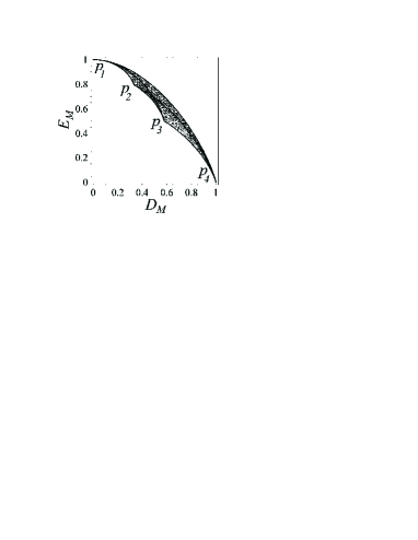
Figure 1: Numerically determined domain in the $D_{M}-E_{M}$ plane corresponding to all physically realizable polarization scattering processes. The solid curves are the analytically obtained bounds. The four cusp points $p_{1}=(0,1)$, $p_{2}=(1/3,\log_{4}3)$, $p_{3}=(1/\sqrt{3},1/2)$, $p_{4}=(1,0)$ separate different polarization scattering processes, as described in the text.

The boundary of this domain is formed by the curves $\mathcal{C}_{ij}$ ($i,j=1,\ldots,4$), joining the points $(p_{i}\rightarrow p_{j})$. The analytical expressions for these curves are

$$E(n,f)=-\left[\left(1-nf\right)\log_{4}\left(1-nf\right)+\,nf\log_{4}\left(f\right)\right],$$ (7)

where

$$f_{\pm}=\frac{1}{n+1}\left[1\pm\sqrt{1-\frac{3}{4}\frac{n+1}{n}(1-D_{M}^{2})}\right].$$ (8)

The links between the functions $E(n,f)$ and the curves $\mathcal{C}_{ij}$ are given in Table I where we have defined $E_{13}=-(1-\mu)\log_{4}(\frac{1-\mu}{2})-\mu\log_{4}(\frac{\mu}{2})$.

Table 1: List of the analytical curves (continuous lines) in Fig. 1. The second column refers to the equations generating the corresponding curves, while the third column gives the eigenvalues of $H$. The first four curves form the boundary of the physical domain; the last two represent inside curves.

Curve		Generating equation		Eigenvalues of $H$
$\mathcal{C}_{12}$		$E(3,f_{+})$		$\{\lambda,\mu,\mu,\mu\}$
$\mathcal{C}_{23}$		$E(2,f_{+})$		$\{\lambda,\mu,\mu,0\}$
$\mathcal{C}_{34}$		$E(1,f_{\pm})$		$\{\lambda,\mu,0,0\}$
$\mathcal{C}_{14}$		$E(3,f_{-})$		$\{\lambda,\mu,\mu,\mu\}$
$\mathcal{C}_{13}$		$E_{13}$		$\{\lambda,\lambda,\mu,\mu\}$
$\mathcal{C}_{24}$		$E(2,f_{-})$		$\{\lambda,\mu,\mu,0\}$

The curve $\mathcal{C}_{14}$ is special in the sense that it sets an upper bound for the entropy of any scattering medium. We find numerically that the value of the entropy on this curve is very well approximated by

$$E_{M}^{\mathrm{cr}}\sim\left(1-D_{M}^{2}\right)^{\gamma},$$ (9)

where $\gamma\cong 0.862$, which is, interestingly, almost equal to $e/\pi$. Then, for all depolarizing scattering media the condition $E_{M}\lesssim E_{M}^{\mathrm{cr}}$ must be satisfied. It is interesting to note that a purely depolarizing scattering medium (with diagonal Mueller matrix) leads to $E_{M}\cong E_{C}$. By using thermodynamics language, one may interpret Fig. 1 as a polarization “state diagram” where different phases of a generic scattering medium, characterized by different symmetries of the corresponding Mueller matrices, are separated by the curves $\mathcal{C}_{ij}$. It is worth to note again that there is nothing inherently quantum in the above derivation of the physical bounds Eq. (7), therefore these results have validity both in the classical and in the quantum regime.

Random matrix approach

We have checked the validity of the theory outlined above, for scattering media in the regime of applicability of the random-matrix theory (RMT) Mehta (1991). Random media, either disordered media DOP or chaotic optical cavities A. Aiello and M. P. van Exter and J. P. Woerdman (2003), can be represented by ensembles Kim et al. (1987). The transmission of polarized light through a random medium may decrease the degree of polarization in a way that depends on the number $N$ of the detected modes via Eq. (2). Under certain conditions, RMT can account for a statistical description of the light scattering by random media Beenakker (1997); Guhr et al. (1998). Let $\psi_{\lambda}(\mathbf{k})$ be the complex probability amplitude that a photon is scattered in the state $|\mathbf{k},\lambda\rangle$. Then, according to RMT, the real and the imaginary parts of the scattering amplitudes $\psi_{\lambda}(\mathbf{k})$ are independent Gaussian random variables with zero mean and variance that can be fixed to $1$. The assumption of independent variables is justified since usually the set $\psi^{\prime\prime}$ of the detected modes is much smaller than the set $\psi^{\prime}$ of the all scattered modes Vel . Let us suppose now that the impinging photon is in the pure state $|\mathbf{k}_{0},\lambda_{0}\rangle$. In this case $\psi_{\lambda}(\mathbf{k})=\mathcal{T}_{\lambda\lambda_{0}}(\mathbf{k},\mathbf{k}_{0})$ and the statistical distribution of the $M_{\mu\nu}$’s can be numerically calculated accordingly to Eqs. (2-3). In this way we have calculated the ensemble-averaged polarization entropy $\langle E_{M}\rangle$ and depolarization index $\langle D_{M}\rangle$ of the medium, as functions of $N$ for the case in which the angular aperture of the detector is so small that $W_{ij}(\mathbf{k})\simeq\delta_{ij}$. The results are shown in Fig. 2 for the cases of a generic scattering medium ($\mathcal{T}_{\lambda\lambda_{0}}(\mathbf{k},\mathbf{k}_{0})$ unconstrained) and of a polarization-conserving medium ($\mathcal{T}_{\lambda\lambda_{0}}(\mathbf{k},\mathbf{k}_{0})\propto\delta_{\lambda\lambda_{0}}$). The last case is realized when the geometry of the scattering process is confined in a plane. As one can see, for both cases RMT results cover only a small part of the ($E_{M},D_{M}$) diagram; however, the numerical data are consistent with the analytical bounds given by Eq. (7).

Figure 2: RMT results for the ensemble-averaged polarization entropy $\langle E_{M}\rangle$ as function of the ensemble-averaged depolarization-index $\langle D_{M}\rangle$ for generic (dark squares) and polarization-conserving (open squares) scattering processes. In both cases each point correspond to a given number $N$ of detected modes. When $N$ increases from $1$ to $30$, points move from the bottom to the top of the figure. The solid lines are the analytical bounds of Fig. 1.

Conclusions

In summary, we have studied the scattering of light by optically random media, from a polarization point of view. To this end we have first extended the Mueller-Stokes formalism to make it suitable for the description of single-photon scattering processes. Then, after the calculation of the Mueller matrix $M$ characterizing the polarization properties of the scattering medium, we have extracted from $M$ the depolarization index $D_{M}$ and the polarization entropy $E_{M}$. By analyzing the functional relation between $E_{M}$ and $D_{M}$, we have found that the polarization properties of any scattering medium are constrained by some physical bounds. These bounds have an universal character and they hold in both the classical and the quantum regime. Our results provide a deeper insight in the nature of random light scattering by giving an useful tool, both to theoreticians and experimenters, to classify scattering media according to their polarization properties. The use of this tool may be particularly relevant in quantum communication where it is desirable to manipulate and control the polarization of the light Legré et al. (2003). Presently, experiments are in progress in our group to verify this theoretical framework.

- (1) F. C. MacKintosh, J. X. Zhu, D. J. Pine, and D. A. Weitz, Phys. Rev. B 40, 9342 (1989); J. M. Schmitt, A. H. Gandjbakhche, and R. F. Bonner, Appl. Opt. 30,6535 (1992); D. Bicout, C. Brosseau, A. S. Martinez, and J. M. Schmitt, Phys. Rev. E 49, 1767 (1994); S. P. Morgan, M. P. Khong, and M. G. Somekh, Appl. Opt. 36, 1560 (1997); A. H. Hielscher, A. A. Eick, J. R. Mourant, D. Shen, J. P. Freyer, and I. J. Bigio, Opt. Express 1, 441 (1997); A. D. Kim and M. Moscoso, Phys. Rev. E 64, 026612 (2001); A. C. Maggs and V. Rossetto, Phys. Rev. Lett. 87, 253901 (2001); O. Korotkova, M. Salem, and E. Wolf, 233, 225 (2004); A. A. Chabanov, N. P. Trégourès, B. A. van Tiggelen, and A. Z. Genack, Phys. Rev. Lett. 92, 173901 (2004).
- Kliger et al. (1990) D. S. Kliger, J. W. Lewis, and C. E. Randall, Polarized Light in Optics and Spettroscopy (Academic Press, Inc., 1990).
- Gil and Bernabeu (1986) J. J. Gil and E. Bernabeu, Optica Acta 33, 185 (1986).
- Roy-Brehonnet and Jeune (1997) F. L. Roy-Brehonnet and B. L. Jeune, Prog. Quant. Electr. 21, 109 (1997).
- Mandel and Wolf (1995) L. Mandel and E. Wolf, Optical Coherence and Quantum Optics (Cambridge University Press, 1995), 1st ed.
- Born and Wolf (1984) M. Born and E. Wolf, Principles of Optics (Pergamon Press, 1984), sixth ed.
- Picozzi (2004) A. Picozzi, Opt. Lett. 29, 1655 (2004).
- Aiello and Woerdman (2004) A. Aiello and J. P. Woerdman, Phys. Rev. A (2004), (to be published), quant-ph/0404029.
- Berestetskiǐ et al. (1971) V. B. Berestetskiǐ, E. M. Lifshitz, and L. P. Pitaevskiǐ, Relativistic Quantum Theory (Pergamon Press, Oxford, 1971), 1st ed.
- Fano (1957) U. Fano, Rev. Mod. Phys. 29, 74 (1957).
- (11) In fact, is a symbolic shorthand representing a direct sum of block matrices, in the space of the variables . For more details see Aiello and Woerdman (2004).
- Peres (1998) A. Peres, Quantum Theory: Concepts and Methods (Kluwer Academic Publisher, 1998).
- Wehrl (1978) A. Wehrl, Rev. Mod. Phys. 50, 221 (1978).
- Simon (1982) R. Simon, Optics Comm. 42, 293 (1982).
- Anderson and Barakat (1994) D. G. M. Anderson and R. Barakat, J. Opt. Soc. Am. A 11, 2305 (1994).
- Mehta (1991) M. L. Mehta, Random Matrices (Academic Press, San Diego, CA, 1991), 2nd ed.
- A. Aiello and M. P. van Exter and J. P. Woerdman (2003) A. Aiello and M. P. van Exter and J. P. Woerdman, Phys. Rev. E 68, 046208 (2003).
- Kim et al. (1987) K. Kim, L. Mandel, and E. Wolf, J. Opt. Soc. Am. A 4, 433 (1987).
- Beenakker (1997) C. W. J. Beenakker, Rev. Mod. Phys. 69, 731 (1997).
- Guhr et al. (1998) T. Guhr, A. Müller-Groeling, and H. A. Weidenmüller, Phys. Rep. 299, 189 (1998).
- (21) J. L. van Velsen and C. W. J. Beenakker, quant-ph/0403093.
- Legré et al. (2003) M. Legré, M. Wegmüller, and N. Gisin, Phys. Rev. Lett. 91, 167902 (2003).