Criteria for Exact Qudit Universality

Abstract

We describe criteria for implementation of quantum computation in qudits. A qudit is a $d$-dimensional system whose Hilbert space is spanned by states $|0\rangle$, $|1\rangle$, $\ldots$, $|d-1\rangle$. An important earlier work of Mathukrishnan and Stroud MathukrishnanStroud:00 describes how to exactly simulate an arbitrary unitary on multiple qudits using a $2d-1$ parameter family of single qudit and two qudit gates. Their technique is based on the spectral decomposition of unitaries. Here we generalize this argument to show that exact universality follows given a discrete set of single qudit Hamiltonians and one two-qudit Hamiltonian. The technique is related to the $QR$-matrix decomposition of numerical linear algebra. We consider a generic physical system in which the single qudit Hamiltonians are a small collection of $H_{jk}^{x}=\hbar\Omega(|k\rangle\langle j|+|j\rangle\langle k|)$ and $H_{jk}^{y}=\hbar\Omega(i|k\rangle\langle j|-i|j\rangle\langle k|)$. A coupling graph results taking nodes $0$, $\ldots$, $d-1$ and edges $j\leftrightarrow k$ iff $H_{jk}^{x,y}$ are allowed Hamiltonians. One qudit exact universality follows iff this graph is connected, and complete universality results if the two-qudit Hamiltonian $H=-\hbar\Omega|d-1,d-1\rangle\langle d-1,d-1|$ is also allowed. We discuss implementation in the eight dimensional ground electronic states of ⁸⁷Rb and construct an optimal gate sequence using Raman laser pulses.

I Introduction

An important theoretic construct used in the field of quantum information is the qubit. Its utility follows from the simple but significant recognition that all two dimensional subspaces, regardless of the underlying physical system, can be regarded as informationally equivalent. This has made it possible to discuss quantum computation in terms of single qubit and two qubit gates without the need to analyze the specific interactions that realize operations within a physical system or between subsystems. An important issue in this regard is that a necessary condition for efficient quantum computation is the existence of an underlying tensor product structure on the Hilbert space $\mathcal{H}$. If all computation were performed on a single $d=dim(\mathcal{H})$ level system then some physical resource such as space or energy would grow with the dimension of the system Blume-KahoutEtAl:02 . In contrast, the analogous resources grow poly-logarithmically with the dimension when the system is composed of many subsystems. By this argument, a computation performed on qubits $(d=2)$ is in some sense the most efficient foliation of Hilbert space.

Nevertheless, there are compelling reasons to consider computation on qudits with $d>2$. First, most physical implementations encode qubits in a subspace of a larger Hilbert space. Using higher dimensional subspaces already endowed in these systems may be more efficient in terms of the number of interacting gates needed for an algorithm that acts on a Hilbert space of fixed dimension. This is critical for error control because interactions between qudits tend to open channels for interactions with the decohering environment. By contrast, in many physical systems, single qudit control is a well developed technology that can be done with high precision. Second, there is some evidence that the error thresholds for fault tolerant computation improve when the encoding is done with qudits where $d>2$ and prime Aharonov .

Previous work by Brylinski and Brylinski proves the necessary and sufficient criteria for exact qudit universality Brylinski:02 . Exact universality means that any unitary and, by unitary extension to a larger Hilbert space, any quantum process, can be simulated with zero error. The authors show that arbitrary single qudit gates complemented by one entangling two qudit gate is needed. Their method is not constructive. Muthukrishnan and Stroud MathukrishnanStroud:00 give a constructive procedure for an exact simulation of an arbitrary unitary on $n$ qudits using single qudit and two qudit gates. Their approach uses the spectral decomposition of unitaries and involves a gate library consisting of a family of continuous parameter gates. Here we describe an approach that uses the $QR$ decompositions on unitaries to achieve exact universal computation on qudits. This construction has the advantage that the single qudit gates are generated by a fixed set of Hamiltonians that couple pairs of states in the single qudit logical basis. The gates perform rotations, parameterized by one angle, about orthogonal axes within the associated two dimensional subspace. Additionally, our decomposition requires only one fixed two qudit gate, the controlled increment gate $(\mathtt{CINC})$ gate. This gate can be simulated by at most $d-1$ instances of a two-qudit Hamiltonian $H_{int}$ that generates a phase on a single product state of two qudits. Such interactions can be engineered in many atom optical systems.

In this paper, the general results are developed with close contact to the example of computation in the $d=8$ qudit encoded in the ground hyperfine states of ⁸⁷Rb. In Sec. II we describe the construction of single qudit unitaries using the $QR$ decomposition. We introduce a coupling graph to describe how states are connected to each other by physical Hamiltonians. The set of rotation planes may be incomplete, i.e. each state may not be connected to every other state. However, provided the graph is connected, an efficient decomposition can be found. Multiqudit computation is addressed in Sec. III. It is shown that a single two-qudit gate when combined with single qudit gates suffices to generate arbitrary two qudit unitaries and hence completes the requirements for exact universality. In the appendix we show how to convert between the gate library introduced here and the family of gates used in Ref. MathukrishnanStroud:00 . Finally, we conclude with a summary of the results in Sec. IV.

II One-qudit unitaries

We pick a fixed gate library for single qudit operations involving rotations about non orthogonal axes of two dimensional subspaces. Within each subspace $\mathcal{H}_{jk}$, the gates are generated by the two Hamiltonians:

$$H_{jk}^{x}=\hbar\Omega(|j\rangle\langle k|+|k\rangle\langle j|),\quad H_{jk}^{y}=\hbar\Omega(-i|j\rangle\langle k|+i|k\rangle\langle j|).$$ (1)

For convenience of notation, we assume the strength of each coupling is equal to $\Omega$ and leave the time each Hamiltonian is applied as a free parameter. Any unitary in the two dimensional subspace can be written

$$\begin{array}[]{llll}U_{j,k}(\gamma,\phi,\theta)&\equiv&\exp\bigg{[}&-i\gamma(\sin(\theta)\cos(\phi)\big{(}\;|j\rangle\langle k|+|k\rangle\langle j|\;\big{)}\\ &&&+\;\sin(\theta)\sin(\phi)\big{(}-i|j\rangle\langle k|+i|k\rangle\langle j|\;\big{)}\\ &&&+\;\cos(\theta)\big{(}\;|j\rangle\langle j|-|k\rangle\langle k|\;\big{)}\;\bigg{]}\\ &=&&e^{-iH^{x}_{jk}t/\hbar}\;e^{-iH^{y}_{jk}t^{\prime}/\hbar}\;e^{-iH^{x}_{jk}t^{\prime\prime}/\hbar}\end{array}$$ (2)

for the appropriate $t,t^{\prime},t^{\prime\prime}$ using the XYX Euler angle decomposition NielsenChuang:00 . In some cases, the two Hamiltonians in Eq. 1 can be turned on simultaneously. By adjusting the relative strengths of the couplings, one can then realize any rotation about an axis on the equator of the Bloch sphere in the two dimensional subspace. For brevity, we write $U_{jk}(\gamma,\phi)=e^{-i(\cos(\phi)H^{x}_{jk}+\sin(\phi)H^{y}_{jk})\gamma/(\hbar\Omega)}$, where it is understood that if the couplings $H^{x}_{jk},H^{y}_{jk}$ cannot be turned on together then $U_{jk}(\gamma,\phi)$ requires three elementary gates.

Realization of an arbitrary unitary evolution $v\in U(d^{n})$ requires two steps. The first corresponds to a $QR$ decomposition Cybenko:01 of the matrix $v$.

• Using the allowed set of Hamiltonians, we may realize matrices of Givens rotations physically. These are described in the next paragraph. Generically, the $QR$ decomposition writes an invertible $G=UT$, where $U=G_{1}G_{2}\ldots G_{\ell}$ is a product of Givens rotations and hence unitary and $T$ is upper triangular. Note that if $G=V$ is unitary, then so likewise is $T=U^{\dagger}G$, whence $T$ is in this case a diagonal matrix which applies relative phases to computational basis states.

• Using techniques for realizing diagonal computations BullockMarkov:04 , a sequence of Hamiltonians realizing $T$ is constructed.

We next illustrate the idea of a Givens rotation by way of example, retaining $V$ as above. We may choose $U$ a Givens rotation so as to zero the matrix element $(UV)_{d-1,0}$ (where the indices run $0,1,\cdots,d-1$.) Specifically, suppose that

$$U_{d-1,d-2}(\gamma,\phi)=\left(\begin{array}[]{rrrr}I_{d^{n}-2}&&&\\ &\ddots&&\\ &&\cos({\gamma})&-ie^{i\phi}\sin({\gamma})\\ &&-ie^{-i\phi}\sin({\gamma})&\cos({\gamma})\\ \end{array}\right)$$ (3)

Here, we choose the angles $\gamma$, $\phi$ as follows:

$$\begin{array}[]{lcl}\tan{\gamma}&=&|v_{d-1,0}/v_{d-2,0}|\\ \phi&=&\pi/2+\arg(v_{d-2,0})-\arg(v_{d-1,0})\\ \end{array}$$ (4)

where $v_{m,n}$ are the entrees of the unitary $V$. Then letting $v^{\prime}_{\ast\ast}$ denote a changed entry, we obtain:

$$U_{d-1,d-2}V=\left(\begin{array}[]{rrrr}v_{0,0}&v_{0,1}&\cdots&v_{0,d-1}\\ \vdots&\ddots&\cdots&\vdots\\ v^{\prime}_{d-2,0}&\cdots&v^{\prime}_{d-2,d-2}&v^{\prime}_{d-2,d-1}\\ 0&\cdots&v^{\prime}_{d-1,d-2}&v^{\prime}_{d-1,d-1}\\ \end{array}\right)$$ (5)

In the next step, one chooses a unitary $U_{d-1,d-3}$ to zero the matrix element $(U_{d-1,d-2}V)_{d-2,0}$. Continuing carefully in this way allows one to complete the $QR$ decomposition described above by introducing a zero into every entry of the resulting unitary below the diagonal.

II.1 Example: One-qudit Unitaries in ⁸⁷Rb

We begin by describing explicitly the implications of our constructions for an example which is related to but not covered explicitly by earlier work of Mathukrishnan and Stroud MathukrishnanStroud:00 . Specifically, we describe the coupling graph alluded to in the introduction in this case before defining it in general.

Thus, consider the atomic species ⁸⁷Rb per Fig. 1. There are two ground state hyperfine manifolds with total spin $F_{\downarrow}=1$ and $F_{\uparrow}=2$ split in energy by the hyperfine interaction $E_{hf}$. Each manifold consists of $2F+1$ degenerate magnetic sublevels $M_{F}$ for a total of eight distinguishable states. We designate this $d=8$ system a quoctet. The degeneracy can be lifted by applying a longitudinal magnetic field $B_{z}$. For small fields, the resultant Zeeman interaction is linear in the magnetic quantum number: $H_{B}=g_{F}B_{z}M_{F}$, where the Lande $g$ factors satisfy $g_{F_{\downarrow}}=-g_{F_{\uparrow}}$ footnote .

There are several ways to couple the magnetic sublevels including the use of microwave pulses and Raman lasers. These techniques are usually distinguished by the strength of the coupling with respect to the hyperfine interaction. We consider coupling that is weak relative to $E_{hf}$ using a pair of laser beams on Raman resonance between two sublevels at a time. The effective atom-laser Hamiltonian $H_{AL}$ in the subspace $\mathcal{H}_{jk}$ is:

$$H_{ALjk}=\cos(\phi)H^{x}_{jk}+\sin(\phi)H^{y}_{jk}$$ (6)

where $\Omega=|\Omega_{1}\Omega_{2}|/\Delta$ is the product of the individual laser Rabi frequencies divided by the detuning $\Delta$ from the excited state, and $\phi=\phi_{1}-\phi_{2}$ is the relative phase of the two beams. In order to selectively couple two states it is necessary that their energy difference be unique. In the linear Zeeman regime, this can only be accommodated when the two levels reside in different hyperfine manifolds. Additionally, it will be important to minimize spontaneous emission during the pulse sequence by choosing a large detuning $\Delta$ of each laser from the excited states. The allowed couplings are constrained by angular momentum selection rules which dictate the change in magnetic spin quantum number during a single pulse sequence. For detuning $\Delta$ much greater than the excited state hyperfine structure, but less than than the fine structure splitting, the angular momentum selection rules dictate $\Delta M_{F}=0,\pm 1$ and $|F_{\downarrow},0\rangle\nleftrightarrow|F_{\uparrow},0\rangle$. Using two-laser pulses of the appropriate frequency and polarization, the states $|F_{\downarrow},M_{F}\rangle$ and $|F_{\uparrow},M_{F}+\Delta M_{F}\rangle$ where $\Delta M_{F}=0,\pm 1$ can then be coupled together. This is shown schematically in Fig. 1 where states $|2\rangle$ and $|5\rangle$ are coupled by a $\sigma_{+}-\pi$ polarized laser pair.

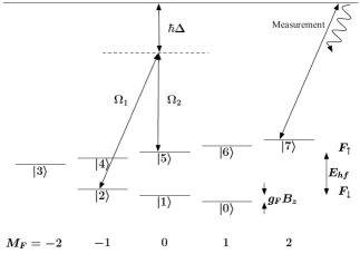
Figure 1: A single $d=8$ qudit (quoctet) encoded in the ground state hyperfine levels of ⁸⁷Rb. A pair of lasers can couple states in different hyperfine manifolds according to the selection rule $\Delta M_{F}=0,\pm 1$. Projective measurements of population in state $|7\rangle$ are made by observing resonant fluorescence on a cycling transition to the excited state. Any pair of states can be coupled by swapping neighbors together pairwise and similarly any state can be measured by swapping to $|7\rangle$.

At this point we pause to comment on the resources necessary for single quoctet compution using Raman pulses. Transitions realizing $\Delta M_{F}=0,\pm 1$ can be achieved by choosing the correct polarizations for the lasers with respect to a quantization axis defined by the magnetic field direction. For a fixed Zeeman splitting, it will be necessary to have lasers tuned to Raman resonance for all the allowed couplings. This may be achievable using a fixed source laser source that is frequency modulated appropriately. Another recourse is to change the magnetic field strength for each pairwise state coupling so that only one laser pair of fixed frequency is necessary. The phase shifts accumulated on the basis states during the change in Zeeman interaction can be accounted for in the gate sequence.

We wish to show that the above set of atom-laser Hamiltonians suffices to construct an arbitrary unitary evolution of the one-quoctet phase space $\mathcal{H}_{1}=\mathbb{C}|0\rangle\oplus\cdots\oplus\mathbb{C}|7\rangle$. Take $V\in U(8)$ as the target one-quoctet evolution, where $U(8)$ is the symmetry group of the inner-product on the Hilbert space (i.e. $VV^{\dagger}=I_{8}$.) The goal then is to decompose $V$ into a sequence of evolutions by these atom laser Hamiltonians:

$$V=\mbox{exp}(iH_{AL}^{1}t_{1}/\hbar)\cdots\mbox{exp}(iH_{AL}^{\ell}t_{\ell}/\hbar)$$ (7)

Additionally, we prefer efficient decompositions, i.e. we wish to use as few laser pulses (as small an $\ell$) as possible. This is sometimes not possible, depending on which states $|j\rangle$, $|k\rangle$ are coupled by an $H_{AL}$. In order to classify when the $QR$ step is possible, we introduce the notion of a coupling graph, by example.

⁸⁷Rb coupling graph: The ⁸⁷Rb coupling graph has vertices labelled by $0,1,\ldots,7$. In addition, consulting Fig. 1, we also allow in the following edges, corresponding to the atom-laser coupled hyperfine states.

$$\big{\{}(0,5),(0,6),(0,7),(1,4),(1,6),(2,3),(2,4),(2,5)\big{\}}$$ (8)

In particular, the edges encode the selection rule for the hyperfine states. The graph is reproduced in Fig. 2. We note for future use that it is connected. Provided the states $|j\rangle$, $|k\rangle$ are coupled, we may produce any determinant-one unitary evolution of $\mathcal{H}_{jk}$ using Eq. 2.

Figure 2: This is the coupling graph for the coupled hyperfine states of ⁸⁷Rb (cf. Fig. 1.) As it is connected, the collection of atom-laser couplings allows for universal one-quoctet computation.

Now note that since the coupling graph is connected, we may in fact sequentially construct a Givens rotation on any $\mathcal{H}_{jk}$. Indeed, even if $|j\rangle$ and $|k\rangle$ are not paired, there exists a sequence $|j_{0}\rangle=|j\rangle,|j_{1}\rangle,|j_{2}\rangle,\ldots,|j_{\ell}\rangle=|k\rangle$ such that each consecutive pair admits atom-laser Hamiltonians. Moreover, taking $\phi=\pi/2,\theta=\pi/2$ in Equation 3 shows that we may use these pairings to swap states up to relative phase. Hence, since we may physically construct some sequence of Hamiltonians for any Givens rotation, we see that the first step of the $QR$ decomposition is possible.

This leaves open the question of efficiency. For example, one might hope that in a graph as highly connected as that for ⁸⁷Rb few or no swaps might be required. This is indeed possible as we now show. It is convenient to reorder the unitary in a logical basis labeled $\{7,0,6,5,3,2,4,1\}$. By successive Givens rotations, one may bring a unitary $V$ to diagonal form column by column where the sequence is chosen so as to not void zeroes created in earlier steps. Each of the columns can be reduced to a single unimodular entry on the diagonal by a sequence of Givens rotations $U_{j,k}$ acting on the two dimensional subspace $\mathcal{H}_{jk}$ as follows O'Leary :

• Column 7 reduction: $U_{4,1}U_{2,4}U_{2,3}U_{5,2}U_{0,5}U_{0,6}U_{7,0}$

• Column 0 reduction: $U_{4,1}U_{2,4}U_{2,3}U_{5,2}U_{0,5}U_{0,6}$

• Column 6 reduction: $U_{2,5}U_{2,3}U_{4,2}U_{1,4}U_{6,1}$

• Column 5 reduction: $U_{4,1}U_{2,4}U_{2,3}U_{5,2}$

• Column 3 reduction: $U_{4,1}U_{2,4}U_{3,2}$

• Column 2 reduction: $U_{4,1}U_{2,4}$

• Column 4 reduction: $U_{4,1}$

Note that in general, constructing $U_{jk}$ requires $2d(j,k)-1$ basic Hamiltonians, where $d(j,k)$ is the distance between $j$ and $k$ in the graph corresponding to the pairing relation. For qudit computation in ⁸⁷Rb using Raman pulses, the graph is sufficiently connected so that the distance is never greater than one in the QR decomposition above. The are a total of $8\times 7/2=28$ gates in the reduction to diagonal form. Each gate $U_{j,k}\in SU(2)$ has two parameters so this gives 56 parameters. An arbitrary $u\in SU(d)$ requires $d^{2}-1$ parameters so the additional 7 parameters correspond to seven relative phases left on the diagonal.

II.2 Relative Phases

The goal of this section is to show that should the Hamiltonian graph be connected and $T=\sum_{j=0}^{d-1}\mbox{e}^{i\varphi_{j}}|j\rangle\langle j|$ be a diagonal element of $U(d)$, then we may realize $T$ with the allowed Hamiltonians $H^{x}_{jk}$, $H^{y}_{jk}$. In fact, we only need to construct $T$ up to a global phase so we can simulate $T^{\prime}=e^{i\phi_{d-1}}T$. We first note that although it is not explicitly an allowed Hamiltonian, we may for any $(j,k)$-edge within the coupling graph simulate the effect of $H^{z}_{jk}=\hbar\Omega(|j\rangle\langle j|-|k\rangle\langle k|)$. Indeed, for any fixed angle $\gamma$ we have

$$e^{-iH^{z}_{jk}\gamma/(\hbar\Omega)}=U_{j,k}(-\pi/4,\pi/2)U_{j,k}(\gamma,0)U_{j,k}(\pi/4,\pi/2).\;$$ (9)

The goal then is to find a sequence of $z$ rotations that simulates $T^{\prime}$:

$$\prod_{l=1}^{p}\exp(-iH^{z}_{j_{l}k_{l}}t_{l}/\hbar)=T^{\prime}\;$$ (10)

Given that the coupling graph is connected, choose a subset $S$ of $d-1$ edges $\lambda^{z}_{jk}=|j\rangle\langle j|-|k\rangle\langle k|$ that leave the graph connected. We can represent the elements of $S$ as vectors in a $d$ dimensional real vector space spanned by the orthonormal vectors $\{e_{j}\}$, i.e. $\lambda^{z}_{jk}=e_{j}-e_{k}$. We then construct a $(d-1)\times d$ matrix $M$ out of the row vectors in $S$: $M=\{\lambda^{z}_{0k_{0}},\lambda^{z}_{1k_{1}},\ldots\lambda^{z}_{d-2k_{d-2}}\}$. The appropriate timings $t_{j}$ in Eq. 10 necessary to simulate $T^{\prime}$ are given by solutions to the matrix equation $M\vec{\theta}=\vec{\phi}$, where $\vec{\theta}=\Omega\{t_{0},\ldots t_{d-2}\}$ and $\vec{\phi}=\{\phi_{0},\ldots\phi_{d-2}\}$. The angle $\phi_{d-1}=0$ for the unitary $T^{\prime}$ by assumption. It is easily verified by Gaussian elimination that the dimension of the row space of $M$ is $d-1$, thus there is a unique solution to the vector $\vec{\theta}$.

The result is that any diagonal unitary can be simulated up to a global phase using $3\times(d-1)$ gates from the gate library. This sequence can be reduced by a factor of three if $z$ rotations can be implemented directly without conjugation. Further, all the Hamiltonians $H_{jk}^{z}$ are diagonal and hence commute, so $z$ rotations that act on disjoint subspaces can be implemented in parallel using additional control resources.

II.3 One-qudit universality for generic coupling graphs

We found that for computation in the ⁸⁷Rb quoctet, a single qudit unitary could be brought to diagonal form using the fewest possible Givens rotations. This is not peculiar to that system but is in fact possible for any system with a connected coupling graph.

Lemma II.1 (O'Leary )

Given a $d$-node coupling graph ${\cal{G}}$ of allowed Givens rotations, then any $U\in SU(d)$ can be brought to diagonal form using $d(d-1)/2$ allowed rotations if and only if ${\cal{G}}$ is connected.

Proof: Suppose ${\cal{G}}$ is connected. Form any spanning tree for it, and renumber the nodes so that the path from node $d$ (the root of the tree) to any node $j$ passes through no node numbered lower than $j$; such a numbering can be constructed by successively deleting leaf nodes and numbering in order of deletion. (For ⁸⁷Rb, we formed the tree by breaking the edge between nodes 6 and 1 and used the logical basis ordering $\{7,0,6,5,3,2,4,1\}$.) At the $j$th step ($j=1,\dots,d-1$), create the tree ${\cal{T_{j}}}$, rooted at node $j$, from the portion of the spanning tree defined by nodes $j,\dots,d$. (Note that ${\cal{T_{j}}}$ is connected due to the way we numbered the nodes.) Then, until only the root of ${\cal{T_{j}}}$ remains, choose a leaf $k$, use a rotation defined by its edge to eliminate element $(k,j)$ of $U$, and delete node $k$ from ${\cal{T_{j}}}$. The result of applying these steps is an upper triangular matrix (and therefore, since $U$ is unitary, a diagonal matrix) computed by using $d(d-1)/2$ allowed rotations.

Suppose ${\cal{G}}$ is not connected and consider a matrix $U\in SU(d)$ that has no zero elements. Choose an arbitrary node to call node $1$. Then we can at best eliminate all but one of the nonzeros in column 1 of the disconnected piece, but there is no allowed rotation that will eliminate the last nonzero. Repeating the argument for each choice of node $1$, we conclude that we cannot reduce $U$ to diagonal form using only allowed rotations. $\Box$

III Multi-qudit Universaility

Suppose in addition to being allowed local Hamiltonians $\{H_{jk}^{x,y}\}$ with a connected coupling graph, the physical system also allows for a two-qudit phase Hamiltonian

$$H_{int}=-\hbar\Omega|d-1,d-1\rangle\langle d-1,d-1|.\;$$ (11)

Using known but dispersed techniques BarencoEtAl:95 ; MathukrishnanStroud:00 , we describe a bootstrap which allows for universal quantum computation. Note that due to the standard $QR$ decomposition, it suffices to construct arbitrary two-qudit unitary evolutions MathukrishnanStroud:00 ; Cybenko:01 . In fact arbitrary one-qudit operations controlled on $d-1$, i.e. $\Lambda_{1}(v)=I_{d^{2}-d}\oplus v\in U(d^{2})$ for $v\in U(d)$, suffice.

Before presenting the generic discussion, we describe a particular example of a two-qubit operation which has seen heavy use MathukrishnanStroud:00 . First, we label as $(\oplus 1)$ the self-map of $\mathbb{Z}/d\mathbb{Z}$ which carries $k\mapsto(k+1)\mbox{mod }d$. Then the controlled-increment gate, abbreviated here as CINC, is defined by extending the following rule linearly:

$${\tt CINC}|j,k\rangle=\left\{\begin{array}[]{rr}|j,k\rangle,&j\neq d-1\\ |j,k\oplus 1\rangle,&j=d-1\\ \end{array}\right..$$ (12)

The CINC gate is heavily used in the literature in building a generic $k$-controlled computation $\Lambda_{k}(v)$ MathukrishnanStroud:00 as well as for constructing quantum error correction codes Grassl:03 .

We may explicitly realize CINC from the Hamiltonian $H_{int}=-\Omega|d-1,d-1\rangle\langle d-1,d-1|$ as follows. This discussion uses the group theory notation that for $j_{1},\ldots,j_{\ell}\subset\{0,1,\ldots,d-1\}$, we write $(j_{1}j_{2}\ldots j_{\ell})$ for the cyclic permutation with $j_{1}\mapsto j_{2}$, $j_{2}\mapsto j_{3}$, $\cdots$, $j_{\ell-1}\mapsto j_{\ell}$, $j_{\ell}\mapsto j_{1}$, and all other set elements fixed. The permutation will also be identified implicitly with the associated permutation matrix $\pi_{(j_{1}j_{2}\ldots j_{\ell})}\in U(d)$. Hence, given $(01)(12)\cdots(d-2\;d-1)=\oplus 1$, we see that ${\tt CINC}=\Lambda_{1}[(01)(12)\cdots(d-2\;d-1)]$. The construction of CINC then takes place in the following steps:

• We may write $\mbox{exp}(-iH_{int}\pi/(\hbar\Omega))=\Lambda_{1}(I_{d-2}\oplus\sigma^{z})$.

• We next argue that we may construct $\Lambda_{1}[(j\;j+1)]$. Indeed, first note that using an appropriate single qudit permutation matrix $U_{j,k}$, we may construct $\Lambda_{1}(I_{j}\oplus\sigma^{z}\oplus I_{d-2-j})$ as

  $$\begin{array}[]{lll}\quad\quad\Lambda_{1}(I_{j}\oplus\sigma^{z}\oplus I_{d-2-j})&=&I_{d}\otimes U_{j+2,d-1}(\pi/2,0)\\ &&\Lambda_{1}(I_{d-2}\oplus\sigma^{z})\\ &&I_{d}\otimes U_{j+2,d-1}(-\pi/2,0).\end{array}$$ (13)

  Then

  $$\begin{array}[]{lll}\quad\quad\Lambda_{1}[(j\;j+1)]&=&I_{d}\otimes U_{j+1,j+2}(\pi/4,\pi/2)\\ &&\Lambda_{1}(I_{j}\oplus\sigma^{z}\oplus I_{d-2-j})\\ &&I_{d}\otimes U_{j+1,j+2}(-\pi/4,\pi/2).\end{array}$$ (14)

• This leads to the realization of CINC in a maximum of $d-1$ controlled operations, given that ${\tt CINC}\;=\;\Lambda_{1}(01)\Lambda_{1}(12)\cdots\Lambda_{1}(d-2\;d-1)$.

We finally consider the construction of an arbitrary $\Lambda_{1}(v)$ for $v\in U(d)$. Again using standard Givens arguments, it suffices to construct $\Lambda_{1}[I_{j}\oplus w\oplus I_{d-j-2}]$ for any $w\in U(2)$, $\mbox{det}(w)=1$. Indeed, using the block-wise permutation argument above, $\Lambda_{1}(w\oplus I_{d-2})$ suffices. Now recall (BarencoEtAl:95 , Lemma 5.1) that there exists for any $w$ as above factor matrices $a$, $b$, and $c$ such that $w=a\sigma^{x}b\sigma^{x}c$ while $I_{2}=abc$. Hence

$$\Lambda_{1}(w\oplus I_{d-2})\ =\ (I_{d}\otimes a)\Lambda_{1}[(01)](I_{d}\otimes b)\Lambda_{1}[(01)](I_{d}\otimes c)$$ (15)

This completes the bootstrap argument for exactly universaility, when the restricted one-qudit Hamiltonian set $\{H_{jk}^{x,y}\}$ is augmented by $H_{int}$.

We showed how the gate CINC can be constructed using the entangling interaction $H_{int}$. In many situations, the interaction between qudits will contain more than one term on the diagonal. For instance, the true Hamiltonian may be

$$H_{int}^{\prime}=\sum_{mn=0}^{d-1}\hbar\Omega_{mn}|mn\rangle\langle mn|.\;$$ (16)

In this case the interaction is entangling iff the following is true Brylinski:02

$$\Omega_{mn}+\Omega_{pq}\neq\Omega_{mq}+\Omega_{pn}+2\pi k\quad\mbox{ for any }m,n,p,q,\mbox{ any }k\in\mathbb{Z}.\;$$ (17)

When the interaction $H_{int}^{\prime}$ is entangling, it is always possible to map it to $H_{int}$ using multiple applications of the coupling conjugated by single qudit gates. In practice, some multiqudit operations may be done more efficiently using $H^{\prime}_{int}$ directly.

There are several proposals for realizing diagonal coupling gates in real physical systems. For example, in trapped atoms possible coupling mechanisms include pairwise interactions via dipole-dipole interactions Brennen:QC1 ; Jaksch:QgateRydberg , and controlled ground state-ground state collisions Jaksch:Qgateoptlatt . The later proposal has been realized recently between atoms trapped in an optical lattice Greiner . These proposals were originally made with the goal of engineering two qubit controlled phase gates. As such, a naïve adaptation to encoding over all magnetic hyperfine levels would fail due to off diagonal couplings between basis states. However, it should be possible to modify one or more proposals to realize a differential shift on a single product state. For instance, in Ref. Stock:Coll it was proposed to realize a quantum gate using the ground state-ground state collisional shift induced by shape resonance. Here one can tune a magnetic field such that a single molecular state is on resonance with a bound motional state of an external trap for both atoms. Because the resonance is dependent on the internal states, a unique phase is accumulated on a single product state. Provided the atoms are sufficiently separated, the other basis state pairs do not interact and a Hamiltonian of the form $H_{int}$ is realized (up to local unitaries.)

IV Conclusions

We have identified the criteria for exact quantum computation in qudits. Our method is constructive and relies on the $QR$ decomposition of unitaries on qudits using a gate library generated by a fixed set of single qudit Hamiltonians and one two qudit entangling gate. Using the concept of a coupling graph we are able to show that universal computation is possible if the nodes (equivalently logical basis states) are connected. Further we give a prescription for efficient single qudit computation by demanding that at each stage of the $QR$ decomposition the graph remain connected. Using the gate library generated by the couplings in Eq. 1 the maximum number of gates is $3d(d+1)/2-3$. The technique for computation is exemplified with a quoctet using the Raman coupled magnetic sublevels of ⁸⁷Rb. It is shown that arbitary single quoctet computation is possible with at most $k=49$ laser pulse sequences. This gate count is optimal and could be reduced to the minimum number $k_{min}=d(d-1)/2=28$ only if one appends the diagonal generators $H_{jk}^{z}$ to the library of couping Hamiltonians.

We note that while the results herein have focused on the construction of unitaries, the ideas can be extended to simulating non-unitary processes such as generalized measurements. Generalized measurements on a system $s$ can be thought of as orthogonal measurements on an extended system $H_{s}\oplus H_{s}^{\perp}$, which may not be orthogonal in $s$ alone. Applications including precision measurement Helstrom:StateEst , quantum communication in the context of entanglement purification Bennett:Entpur , and quantum error correction Preskill:QECreq . To realize this positive operator valued measurement (POVM), one can perform a unitary operation on $H_{s}\oplus H_{s}^{\perp}$ followed by a projective measurement on $H_{s}^{\perp}$ alone. For example, non-orthogonal measurements on a qubit can be realized by appending ancillary qubits, performing unitary operations on the joint system, and measuring the ancillae. The requirement of using two qubit gates can be obviated if the ancillary degrees of freedom come from orthogonal states within the same system. For example, one can use the $d-2$ states of a qudit to implement POVMs on an orthogonal qubit subspace. These ideas are explored in the context of quantum optical systems in Refs. Arnold:01 ; Brennen:01 . The techniques reported here indicate that the requisite operations on the appended Hilbert space can be done efficiently.

Appendix A Connection to earlier multiqudit gate constructions

Mathukrishnan and Stroud have shown MathukrishnanStroud:00 that exact universal computation over qudits can be achieved using a gate library containing a $2d-1$ parameter family of two qudit gates. We show that this family of gates can be simulated using $d-1$ instances of a single parameter two-qudit gate generated by the Hamiltonian $H_{int}$ (Eq. 11).

They begin by writing the unitary $W\in SU(d^{n})$ in its spectral decomposition:

$$W=\sum_{j=0}^{d^{n}-1}e^{i\lambda_{j}}|\lambda_{j}\rangle\langle\lambda_{j}|.$$ (18)

The unitary can then be expressed as the product

$$W=\prod_{j=0}^{d^{n}-1}X_{f}(|\lambda_{j}\rangle)V_{f}(\lambda_{j})X_{f}^{-1}(|\lambda_{j}\rangle),\;$$ (19)

Here the operator $V_{f}(\lambda_{j})$ applies a phase only to a fiducial logical basis state $|f\rangle$,

$$V_{f}(\lambda_{j})=e^{i\lambda_{j}}|f\rangle\langle f|+\sum_{k\neq f}|k\rangle\langle k|,\;$$ (20)

The operator $X_{f}(|\lambda_{j}\rangle)$ is a unitary extension of the map from the fiducial state to an eigenvector of $U$:

$$X_{j}(|\lambda_{j}\rangle)=|\lambda_{j}\rangle\langle f|+\sum_{k\neq f}|\chi_{k}(j)\rangle\langle k|.\;$$ (21)

where $\langle\lambda_{j}|\chi_{k}(j)\rangle=0$ and $\langle\chi_{k}(j)|\chi_{k^{\prime}}(j)\rangle=\delta_{k,k^{\prime}}$. There is a freedom in the choice of the unitary extension by fixing the set of mappings $\{|k\rangle\rightarrow|\chi_{k}(j)\rangle\}$. Notice that arbitrary single qudit operations can be constructed using the spectral decomposition for $n=1$ and choosing the fiducial state to be logical basis state of one qudit. Here we fix $|f\rangle=|d-1\rangle$. The two multiqudit operators Eqs. 20, 21 can be simulated exactly the using single qudit operations and two families of controlled two-qudit operators. The first two-qudit gate defines a one parameter family of controlled-phase gates and is in fact generated directly by $H_{int}$:

$$\Lambda_{1}(V(\phi))=e^{-iH_{int}\phi/(\hbar\Omega)}.\;$$ (22)

The second family of operators is defined $\Lambda_{1}(X(|\psi\rangle))$ and maps $|d-1\rangle\rightarrow|\psi\rangle$ on the target qudit iff the control is in state $|d-1\rangle$ and applies ${\bf 1}$ to the target otherwise:

$$\begin{array}[]{lll}\Lambda_{1}(X(|\psi\rangle))&=&\sum_{k\neq d-1,k^{\prime}}|kk^{\prime}\rangle\langle kk^{\prime}|\\ &&+|d-1\rangle\langle d-1|\otimes(|\psi\rangle\langle d-1|\\ &&+\sum_{k\neq d-1}|\beta_{k}\rangle\langle k|),\end{array}$$ (23)

where $\langle\psi|\beta_{k}\rangle=0$ and $\langle\beta_{j}|\beta_{k}\rangle=\delta_{j,k}$. Because the gate is allowed to implement any unitary extension of $|\psi\rangle_{t}\langle d-1|$, it only depends on the $2d-2$ parameters of the state $|\psi\rangle$ (two parameters are fixed by the norm $\langle\psi|\psi\rangle=1$ and setting the global phase to zero.)

The gate $\Lambda_{1}(X(|\psi\rangle))$ can be simulated exactly with the controlled-phase gate (Eq. 22) and single qudit gates as we now show. First, expand the state $|\psi\rangle$ in the single qudit basis: $|\psi\rangle=\sum_{j=0}^{d-1}c_{j}|j\rangle$, where the global phase is chosen so that $\arg{c_{d-1}}=1$. The conditional mapping $|d-1\rangle\rightarrow|\psi\rangle$ can be realized as a sequence of $d-1$ controlled unitaries that couple two target qudit basis states at a time,

$$\Lambda_{1}(X(|\psi\rangle))=\prod_{j=0}^{d-2}\Lambda_{1}(U_{j,d-1}(\gamma_{j},\phi_{j})),\;$$ (24)

The arguments $(\theta_{j},\phi_{j})$ for each controlled unitary must satisfy the following relations:

$$\begin{array}[]{lll}c_{d-2}&\equiv&\langle d-2|U_{d-2,d-1}|d-1\rangle=-ie^{i\phi_{d-2}}\sin{\gamma_{d-2}}\\ c_{d-3}&\equiv&\langle d-3|U_{d-3,d-1}U_{d-2,d-1}|d-1\rangle\\ &=&\langle d-3|U_{d-3,d-1}|d-1\rangle\\ &&\langle d-1|U_{d-2,d-1}|d-1\rangle\\ &=&-ie^{-\phi_{d-3}}\sin{\gamma_{d-3}}\cos{\gamma_{d-2}}\\ &\vdots&\\ c_{k}&=&-ie^{i\phi_{k}}\sin{\gamma_{k}}\prod_{l=k+1}^{d-2}\cos{\gamma_{l}}\ \ \ (k<d-2).\end{array}$$ (25)

Now it only remains to demonstrate that each controlled rotation $\Lambda_{1}(U_{j,d-1})$ can be simulated with just the controlled phase gate and rotations on the target qudit. A single conjugation suffices:

$$\begin{array}[]{lll}\Lambda_{1}(U_{j,d-1})&=&{\bf 1}\otimes U_{j,d-1}(\gamma_{j}/2+\pi,\phi_{j})\\ &&e^{-iH_{int}\pi/(\hbar\Omega)}{\bf 1}\otimes U_{j,d-1}(-\gamma_{j}/2+\pi,\phi_{j}).\end{array}$$ (26)

Following this construction, $d-1$ controlled phase gates and $d$ single qudit gates suffice to exactly simulate $\Lambda_{1}(X(|\psi\rangle))$.

References

- (1) A. Mathukrishnan and C.R.Stroud Jr., Phys. Rev. A 62, 052309 (2000).
- (2) R. Blume-Kahout, C.M. Caves, I.H. Deutsch, Found. Phys. 32, 1641 (2002).
- (3) D. Aharonov, Presented at Conference on Quantum Information: Entanglement, Decoherence and Chaos, Institute for Theoretical Physics, Santa Barbara, 2001 (unpublished).
- (4) J.-L. Brylinski and R. Brylinski, Mathematics of Quantum Computation, edited by R. Brylinski and G. Chen, CRC Press (2002). quant-ph/0108062.
- (5) M. Nielsen and I. Chuang, Quantum Computation and Quantum Information, Cambridge Univ. Press, 2000.
- (6) G. Cybenko, Reducing quantum computations to elementary unitary operations, Comp. in Sci. and Eng., 27, March/April 2001.
- (7) S.S. Bullock and I.L. Markov, Quant. Info. and Comp. 4, 27 (2004).
- (8) The equality of the Lande-g factors up to a sign is an approximation that neglects the nuclear magneton. For 87Rb this approximation is good to within Steck but for larger nuclei such as 133Cs the error is non-negligible. The correction does not affect the results here.
- (9) D.A. Steck, Rubidium 87 D Line Data, document available online at http://steck.us/alkalidata.
-
(10)
D.P. O’Leary and S.S. Bullock, submitted to
Electronic Transactions in Numerical Analysis,
http://math.nist.gov/SBullock. - (11) A. Barenco et al., Elementary gates for quantum computation, Phys. Rev A, 52 3457 (1995).
- (12) M. Grassl, M. Roetteler, and T. Beth, Int. J. Found. of Comp. Sci., 14, 757 (2003).
- (13) G.K. Brennen, I.H. Deutsch,and C.J. Williams, Phys. Rev. A 65, 022313 (2002).
- (14) D. Jaksch, J.I. Cirac, P. Zoller, S.L. Rolston, R. Cote, and M.D. Lukin, Phys. Rev. Lett. 85, 2208 (2000).
- (15) D. Jaksch, H.J. Briegel, J.I. Cirac, C.W. Gardiner, and P. Zoller, Phys. Rev. Lett. 82 1975 (1999).
- (16) A. Widera, O. Mandel, M. Greiner, S. Kreim, T.W. Hansch, and I. Bloch, Phys. Rev. Lett. 92, 160406 (2004).
- (17) R. Stock, E.L.. Bolda, and I.H. Deutsch, Phys. Rev. Lett. 91, 183201 (2003).
- (18) C.W. Helstrom, Quantum Detection and Estimation Theory (Academic Press, New York, 1976).
- (19) C.H. Bennett, D.P. DiVincenzo, J.A. Smolin, and W.K. Wootters, Phys. Rev. A 54, 3824 (1996).
- (20) J. Preskill, Proc. R. Soc. London Ser. A 454, 385 (1998).
- (21) S. Franke-Arnold, E. Andersson, S.M. Barnett, and S. Stenholm, Phys. Rev. A 63, 052301 (2001).
- (22) G.K. Brennen, Ph.D. Thesis, University of New Mexico (2001).