Field squeeze operators in optical cavities with atomic ensembles

Abstract

We propose a method of generating unitarily single and two-mode field squeezing in an optical cavity with an atomic cloud. Through a suitable laser system, we are able to engineer a squeeze field operator decoupled from the atomic degrees of freedom, yielding a large squeeze parameter that is scaled up by the number of atoms, and realizing degenerate and non-degenerate parametric amplification. By means of the input-output theory we show that ideal squeezed states and perfect squeezing could be approached at the output. The scheme is robust to decoherence processes.

Squeezing can be defined, in a harmonic oscillator, as the reduction of quantum fluctuations in a certain quadrature below the vacuum level, at the expense of increasing them in its canonically conjugate variable MandelWolf . The possibility of manipulating quantum fluctuations was first noticed by Caves et al. Caves , with the aim of precision measurements. Since then, much effort has been devoted to it through theoretical proposals and experimental implementations Wineland . Recently, with the advent of quantum information and communication, entangled squeezed states of the electromagnetic field Lam have led to the realization of continuous variable teleportation Kimble . Also, by improving the yet low squeeze parameters, it is expected that two-mode squeezed states will lead to efficient distribution of entanglement and implementation of quantum channels ClarkKraus . Two-mode (polarization) squeezing has already been realized by means of Kerr nonlinearity in optical fibers Lorenz and with cold atomic clouds in optical cavities Giacobino . Recently, theoretical and experimental developments relating atomic ensembles and quantum information devices, like entanglement Polzik and exchange of information between light and atomic states Hammerer , have raised justified expectations on related topics. However, to our knowledge, an effective and tunable field squeeze operator MandelWolf has not yet been proposed or realized.

In this letter, we present a method that produces single and two-mode squeeze operators, decoupled from the atomic degrees of freedom, acting on a cavity containing an atomic ensemble. The squeeze parameters scale up with the interaction time and with the number of atoms present in the interaction region of the cavity. This method shows to be robust against decoherence processes, like spontaneous emission, and does not require strong coupling regime or strong atomic localization. Furthermore, we use the input-output formalism to show that it is possible to generate two-photon coherent states Yuen (or ideal squeezed states idealCaves ) and to approach perfect squeezing at the output field, allowing the study of their features in a wide range of parameters.

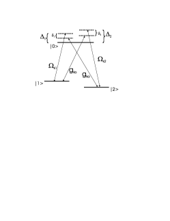
Figure 1: Each three-level atom is driven with two classical fields, with frequencies $\nu_{1}$ and $\nu_{2}$, establishing a couple of Raman laser systems through two cavity modes.

Our model consists of an ensemble of $N$ identical three-level atoms inside an optical cavity Molmer ; Giacobino . For the sake of generality, we assume that the atoms occupy random positions $\mathbf{r}_{k}$ ($k=1,...,N$) along the spatial distribution of two cavity modes, $u_{a}(\mathbf{r})$ and $u_{b}(\mathbf{r})$. Each atom interacts with these two quantized modes and with two properly tuned lasers, as sketched in Fig. 1, yielding a couple of independent Raman laser systems. The associated Hamiltonian can be written as

$$H=H_{\mathrm{0}}+H_{\mathrm{int}},$$ (1)

with

$$H_{\mathrm{0}}=\hbar\omega_{a}a^{{\dagger}}a+\hbar\omega_{b}b^{{\dagger}}b+\hbar\sum\limits_{k=1}^{N}\sum\limits_{i=0}^{2}\omega_{i}\left|i\right\rangle_{k}\left\langle i\right|,$$ (2)

and

$$H_{\mathrm{int}} = \sum\limits_{k=1}^{N}\left\{\left(\Omega_{k1}\left|0\right\rangle_{k}\left\langle 1\right|e^{-i\nu_{1}t}+\Omega_{k1}^{\ast}\left|1\right\rangle_{k}\left\langle 0\right|e^{i\nu_{1}t}\right)\right.$$ (3)

$$+\left(\Omega_{k2}\left|0\right\rangle_{k}\left\langle 2\right|e^{-i\nu_{2}t}+\Omega_{k2}^{\ast}\left|2\right\rangle_{k}\left\langle 0\right|e^{i\nu_{2}t}\right)$$

$$+\left(g_{ka}\left|0\right\rangle_{k}\left\langle 2\right|a+g_{ka}^{\ast}\left|2\right\rangle_{k}\left\langle 0\right|a^{{\dagger}}\right)$$

$$+\left(g_{kb}\left|0\right\rangle_{k}\left\langle 1\right|b+g_{kb}^{\ast}\left|1\right\rangle_{k}\left\langle 0\right|b^{{\dagger}}\right)\}.$$

Here, $a$ ($a^{\dagger}$) and $b$ ($b^{\dagger}$) are the annihilation (creation) operators associated with two cavity modes, with frequencies $\omega_{a}$ and $\omega_{b}$, respectively. Atomic states $|i\rangle$ ($i=0,1,2$) have Bohr frequencies $\omega_{i}$ and are coupled in two simultaneous Lambda configurations LawEberly . Atomic transitions $|1\rangle\leftrightarrow|0\rangle$ and $|2\rangle\leftrightarrow|0\rangle$ are coupled through classical fields with coupling constants $\Omega_{k1}=\Omega_{1}v_{1}(\mathbf{r}_{k})$ and $\Omega_{k2}=\Omega_{2}\,v_{2}(\mathbf{r}_{k})$, and also through the two cavity modes, $b$ and $a$, with coupling constants $g_{kb}=g_{b}\,u_{b}(\mathbf{r}_{k})$ and $g_{ka}=g_{a}\,u_{a}(\mathbf{r}_{k})$, respectively.

In the interaction picture, the associated Hamiltonian reads

$$H_{\mathrm{I}} \!\!=\!\! \hbar\sum\limits_{k=1}^{N}\left\{\Omega_{k1}\left|0\right\rangle_{k}\left\langle 1\right|e^{-i\Delta_{1}t}+\Omega_{k1}^{\ast}\left|1\right\rangle_{k}\left\langle 0\right|e^{i\Delta_{1}t}\right.$$ (4)

$$+\Omega_{k2}\left|0\right\rangle_{k}\left\langle 2\right|e^{-i\Delta_{2}t}+\Omega_{k2}^{\ast}\left|2\right\rangle_{k}\left\langle 0\right|e^{i\Delta_{2}t}$$

$$+g_{ka}\left|0\right\rangle_{k}\left\langle 2\right|ae^{-i\tilde{\Delta}_{1}t}+g_{ka}^{\ast}\left|2\right\rangle_{k}\left\langle 0\right|a^{{\dagger}}e^{i\tilde{\Delta}_{1}t}$$

$$\left.+g_{kb}\left|0\right\rangle_{k}\left\langle 1\right|be^{-i\tilde{\Delta}_{2}t}+g_{kb}^{\ast}\left|1\right\rangle_{k}\left\langle 0\right|b^{{\dagger}}e^{i\tilde{\Delta}_{2}t}\right\},$$

where $\Delta_{i}=\omega_{i}-\omega_{0}+\nu_{i}$, $\tilde{\Delta}_{i}=\Delta_{i}-\delta_{i}$ ($i=1,2$), and also $\tilde{\Delta}_{1}=\omega_{2}-\omega_{0}+\omega_{a}$, $\tilde{\Delta}_{2}=\omega_{1}-\omega_{0}+\omega_{b}$. We consider dispersive detunings $\{|(\Delta_{i}-\Delta_{j})|,|(\tilde{\Delta}_{i}-\tilde{\Delta}_{j})|,|(\tilde{\Delta}_{i}-\Delta_{j})|,|\Delta_{i}|,|\tilde{\Delta}_{i}|\}\gg\{|\delta_{i}|,|g_{ka}|,|g_{kb}|,|\Omega_{k1}|,|\Omega_{k2}|\}$, with $i=1,2$ ($i\neq j$), $k=1,...,N$. Then, we eliminate adiabatically level $|0\rangle$ and obtain the effective Hamiltonian

$$\!\!\!\!\!\!H_{\mathrm{II}} \!\!\!=\!\!\! \hbar\sum_{k}\bigg{[}\left(\frac{|g_{kb}|^{2}}{\tilde{\Delta}_{2}}b^{{\dagger}}b+\frac{|\Omega_{k1}|^{2}}{\Delta_{1}}\right)\left|1\right\rangle_{k}\left\langle 1\right|$$ (5)

$$+\left(\frac{|g_{ka}|^{2}}{\tilde{\Delta}_{1}}a^{{\dagger}}a+\frac{|\Omega_{k2}|^{2}}{\Delta_{2}}\right)\left|2\right\rangle_{k}\left\langle 2\right|$$

$$+\left(\frac{\Omega_{k1}g_{ka}^{\ast}}{\Delta_{1}}a^{{\dagger}}e^{-i\delta_{1}t}+\frac{g_{kb}\Omega_{k2}^{\ast}}{\Delta_{2}}be^{i\delta_{2}t}\right)\sigma_{k}^{-}\,$$

$$+\left(\frac{\Omega_{k2}g_{kb}^{\ast}}{\Delta_{2}}b^{{\dagger}}e^{-i\delta_{2}t}+\frac{g_{ka}\Omega_{k1}^{\ast}}{\Delta_{1}}ae^{i\delta_{1}t}\right)\sigma_{k}^{+}\bigg{]},$$

where $\sigma_{k}^{+}=\left|1\right\rangle_{k}\left\langle 2\right|$ and $\sigma_{k}^{-}=\sigma_{k}^{+\dagger}=\left|2\right\rangle_{k}\left\langle 1\right|$ are raising and lowering atomic operators, respectively. For simplicity, we have discarded terms that require an initial population of level $|0\rangle$.

By making the unitary transformation $e^{iAt/\hbar}$, with

$$A=\hbar\widetilde{\delta}(a^{{\dagger}}a+b^{{\dagger}}b)+\hbar\sum_{k}(\frac{|\Omega_{k1}|^{2}}{\Delta_{1}}\left|1\right\rangle_{k}\left\langle 1\right|+\frac{|\Omega_{k2}|^{2}}{\Delta_{2}}\left|2\right\rangle_{k}\left\langle 2\right|),$$ (6)

where $\ \widetilde{\delta}=(\delta_{2}+\delta_{1})/2$ , we obtain the new Hamiltonian

$$H_{\mathrm{III}} = \hbar\{-\tilde{\delta}(a^{{\dagger}}a+b^{{\dagger}}b)+$$ (7)

$$\sum_{k}(\frac{|g_{ka}|^{2}}{\tilde{\Delta}_{1}}a^{{\dagger}}a\left|2\right\rangle_{k}\left\langle 2\right|+\frac{|g_{kb}|^{2}}{\tilde{\Delta}_{2}}b^{{\dagger}}b\left|1\right\rangle_{k}\left\langle 1\right|$$

$$+[(\tilde{\Omega}_{ka}a+\tilde{\Omega}_{kb}^{\ast}b^{{\dagger}})e^{-i\delta_{k}t}\sigma_{k}^{+}+\mathrm{H.c.}])\}.$$

Here, $\delta_{k}=(\delta_{2}-\delta_{1})/2+|\Omega_{k2}|^{2}/\Delta_{2}-|\Omega_{k1}|^{2}/\Delta_{1}$, and $\tilde{\Omega}_{ka}=\Omega_{k1}^{\ast}g_{ka}/\Delta_{1},$ $\tilde{\Omega}_{kb}=\Omega_{k2}^{\ast}g_{kb}/\Delta_{2}$.

We make now the unitary transformation $e^{iV(t)/\hbar}$, with $V(t)=-i\hbar\sum_{k}\sigma_{k}^{-}\left(\tilde{\Omega}_{ka}^{\ast}a^{{\dagger}}+\tilde{\Omega}_{kb}b\right)(e^{i\delta_{k}t}-1)/\delta_{k}+\mathrm{H.c.}$ , assuming $|\delta_{k}|t\gg 1$, $|\delta_{k}|\gg\{|\tilde{\Omega}_{ka}|,|\tilde{\Omega}_{kb}|,\frac{|g_{ka}|^{2}}{\tilde{\Delta}_{1}},\frac{|g_{kb}|^{2}}{\tilde{\Delta}_{2}},\tilde{\delta}\}$, and obtain

$$\!\!\!\!\!H_{\mathrm{IV}} \!\!\!=\!\hbar\{-\tilde{\delta}(a^{{\dagger}}a\!+\!b^{{\dagger}}b)+\!\!\sum_{k}(\frac{|\tilde{\Omega}_{kb}|^{2}}{\delta_{k}}|2\rangle_{k}\langle 2|\!-\!\frac{|\tilde{\Omega}_{ka}|^{2}}{\delta_{k}}|1\rangle_{k}\langle 1|$$ (8)

$$+\frac{|g_{ka}|^{2}}{\tilde{\Delta}_{1}}a^{{\dagger}}a\left|2\right\rangle_{k}\left\langle 2\right|+\frac{|g_{kb}|^{2}}{\tilde{\Delta}_{2}}b^{{\dagger}}b\left|1\right\rangle_{k}\left\langle 1\right|$$

$$-\sigma_{k}^{z}\,[\,\frac{|\tilde{\Omega}_{ka}|^{2}}{\delta_{k}}a^{{\dagger}}a+\frac{|\tilde{\Omega}_{kb}|^{2}}{\delta_{k}}b^{{\dagger}}b$$

$$+\frac{\tilde{\Omega}_{ka}^{\ast}\tilde{\Omega}_{kb}^{\ast}}{\delta_{k}}a^{{\dagger}}b^{{\dagger}}+\frac{\tilde{\Omega}_{ka}\tilde{\Omega}_{kb}}{\delta_{k}}ba])\},$$

where $\sigma_{k}^{z}=|1\rangle_{k}\langle 1|-|2\rangle_{k}\langle 2|$. We assume that all atoms are initially in the ground state, $\Pi_{k}|2\rangle_{k}$, which allows us to replace $\sigma_{k}^{z}$ by $-1$ in Eq. (8). We require the condition

$$\tilde{\delta}=\sum_{k}(\frac{|\tilde{\Omega}_{ka}|^{2}}{\delta_{k}}+\frac{|g_{ka}|^{2}}{\tilde{\Delta}_{1}})=\sum_{k}\frac{|\tilde{\Omega}_{kb}|^{2}}{\delta_{k}},$$ (9)

which can be easily satisfied by adjusting properly the classical field strengths $\Omega_{k1}/\Omega_{k2}$ and the ratio $\Delta_{1}/\Delta_{2}$ . Then, up to a constant term, $H_{\mathrm{IV}}$ can be rewritten as

$$H_{\mathrm{IV}}=\hbar(\Omega a^{{\dagger}}b^{{\dagger}}+\Omega^{\ast}ba),$$ (10)

where $\Omega=\sum_{k}\tilde{\Omega}_{ka}^{\ast}\tilde{\Omega}_{kb}^{\ast}/\delta_{k}.$ Therefore, the time evolution operator in the Schrödinger picture reads

$$U(\tau)\simeq e^{-i\tilde{H}_{0}\tau/\hbar}U^{\mathrm{ND}}(\tau),$$ (11)

where we made $e^{iV(t)/\hbar}\simeq 1$, consistently with approximations made before, and defined $\tilde{H}_{0}$ $=H_{0}+A$ and

$$U^{\mathrm{ND}}=e^{(\xi^{\ast}ab-\xi\,a^{\dagger}b^{\dagger})}.$$ (12)

Here, explicitly, $\xi=\tau\sum_{k}\Omega_{k1}\Omega_{k2}g_{ka}^{\ast}g_{kb}^{\ast}/(\delta_{k}\Delta_{1}\Delta_{2})$ is a squeeze parameter that scales with the number of atoms $N$, $\tau$ being the interaction time. The time evolution operator in Eq. (12) is a unitary two-mode squeeze operator that is decoupled from the atomic degrees of freedom, producing two-mode squeezing on any initial field state. In particular, given that at room temperature an optical cavity field is in the vacuum state, a two-mode squeezed vacuum will be naturally produced. Eq. (12) corresponds to a physical implementation of a non-degenerate (ND) parametric oscillator in the domain of cavity QED and atomic clouds. Implementation of a degenerate (D) parametric oscillator is straightforward if we consider mode $b$ identical to mode $a$, yielding $U^{\mathrm{D}}=e^{(\xi^{\ast}a^{2}-\xi\,a^{\dagger 2})}$.

At this point, we will make some experimental considerations, stressing that each physical implementation will require specific adaptations. In fact, to assure a large squeezing in a fixed quadrature of the cavity mode, all atoms in the interaction volume should contribute coherently. Let us consider an optical cavity with cylindrical symmetry around the z-axis with $u_{a}(\mathbf{r}_{k})\sim\sin(q_{a}z_{k})f_{a}(\rho_{k})e^{im\varphi_{k}}$, $u_{b}(\mathbf{r}_{k})\sim\sin(q_{b}z_{k})f_{b}(\rho_{k})e^{-im\varphi_{k}}$. We choose the classical fields to counterpropagate perpendicular to the axis of the cavity, so as to warrant a coherent atomic contribution in the effective interaction volume when $d|q_{a}-q_{b}|\ll 1$ and $w|\nu_{1}-\nu_{2}|/c\ll 1$, $d$ being the beam widths and $w\sim d$ the waist of the modes. These conditions relax the typical requirement of atomic localization inside a wavelength, and can be easily satisfied, in general, if the two lower levels are separated by a small splitting compared to optical frequencies.

We consider a low density vapor of ${}^{85}\mathrm{Rb}$ in an optical cavity. The two lower levels $|1\rangle$ and $|2\rangle$ are the ground state $(5S_{1/2})$ hyperfine levels ($F=2$ and $F=3$), separated by $3$GHz, while level $|0\rangle$ is the first excited state $(5P_{3/2})$, yielding optical transitions of $780\mathrm{nm}$. Using the cavity parameters of Ref. RubidiumRempe , we have $w\sim 35\mu\mathrm{m}$, homogeneous laser beams of width $d\sim 50\mu\mathrm{m}$, and an interaction volume of $\sim 10^{-7}\mathrm{cm^{3}}$. We choose, for example, $\Omega_{k1}$ $\sim 100g$, $\Omega_{k2}=\Omega_{k1}/10$, $\Delta_{2}=2\Delta_{1}$, $g_{a}\sim g_{b}=g$, and dispersive condition $\Delta_{1}/\Omega_{k1}=100$. These values and Eq. (9) are enough to estimate all relevant parameters, while satisfying strictly all requirements to derive $H_{\rm IV}$ of Eq. (10). In particular, we calculate $\delta_{k}=-(1-1/400)g$, $\delta_{1}=-3g/400$, $\delta_{2}=-g/80$, $\tilde{\delta}=-g/100$, an effective coupling $\Omega=-g/5$, and $N=4\times 10^{4}$, corresponding to a density of $\lesssim 10^{12}/\mathrm{cm^{3}}$ (small enough to prevent coherence losses due to collisions). This is just a rather conservative set of parameters, for a chosen experimental setup RubidiumRempe , from a wide range of possibilities.

The maximal value of the squeeze parameter in Eq. (12), for the same example, is $|\xi|_{max}\sim(|g|/5)\tau_{\rm diss}$, with $\tau_{\mathrm{diss}}\equiv 1/\kappa{\bar{n}}$, $\kappa$ being the cavity decay rate and ${\bar{n}}$ the mean number of cavity photons. Given that for squeezed vacuum $\bar{n}=\sinh^{2}(2|\xi|)$, and with a conservative $|g|/\kappa\sim 5$, the present scheme should be able to produce field squeezing $\sim 70\%$, which is a competitive value when compared with recent achievements Giacobino . However, as we will see in the second part of the manuscript, the condition $|\Omega|=|g|/5=\kappa$ is enough to approach, theoretically, perfect squeezing at the cavity output.

The noisy effect of spontaneous emission will be negligible here, for typical values of individual atomic emission rate $\Gamma$ and in presence of a large number of atoms. It is possible to estimate that even for a high squeeze parameter $\xi$, very few photons, $N_{\Gamma}\sim N\Gamma(\Omega_{k}/\Delta)^{2}\tau_{\mathrm{diss}}\ll N$, would be spontaneously emitted from the whole cloud. For the realistic parameters of our previous example, $N_{\Gamma}<1\ll N\sim 4\times 10^{4}$.

Now, we will concentrate on the squeezing properties of the outgoing cavity field. We recall that the output field that has been considered for diverse applications and can be measured through standard optical procedures Giacobino .

We consider the input-output theory, successfully applied to the study of the parametric amplifier GardinerZoller , for the case of two cavity modes driven by the effective nonlinear interaction in Eq. (12) and by external (axial) laser fields. The classical fields drive cavity modes $a$ and $b$ with strengths $\epsilon_{a}$ and $\epsilon_{b}$, respectively. We assume that each cavity mode interacts with an independent heat bath such that, in the Markov approximation, the following coupled Langevin equations are produced

$$\dot{a} = -i\epsilon_{a}^{\ast}+\frac{\Omega}{2}\,b^{{\dagger}}-\frac{\kappa_{a}}{2}a-\sqrt{\kappa_{a}}\,c_{\mathrm{in}}(t)$$

$$\dot{b} = -i\epsilon_{b}^{\ast}+\frac{\Omega}{2}\,a^{{\dagger}}-\frac{\kappa_{b}}{2}b-\sqrt{\kappa_{b}}\,d_{\mathrm{in}}(t).$$ (13)

Here, $c_{\mathrm{in}}(t)$ and $d_{\mathrm{in}}(t)$ are annihilation operators associated with the input fields, $\kappa_{a}$ and $\kappa_{b}$ are the cavity decay rates of modes $a$ and $b$, and we have considered $\Omega\rightarrow i\Omega/2$ ($\Omega$ real) to match standard notation GardinerZoller . Then, Eqs. (13) can be rewritten as

$$\dot{a^{\prime}} = \frac{\Omega}{2}\,{b^{\prime}}^{{\dagger}}-\frac{\kappa_{a}}{2}{a^{\prime}}-\sqrt{\kappa_{a}}\,c_{\mathrm{in}}(t)$$

$$\dot{b^{\prime}} = \frac{\Omega}{2}\,{a^{\prime}}^{{\dagger}}-\frac{\kappa_{b}}{2}b^{\prime}-\sqrt{\kappa_{b}}\,d_{\mathrm{in}}(t),$$ (14)

where the transformations

$$a = a^{\prime}+\alpha_{0}$$

$$b = b^{\prime}+\beta_{0},$$ (15)

with $\alpha_{0}=2i(\kappa_{b}\epsilon_{a}^{\ast}-\Omega\epsilon_{b})/(\Omega^{2}-\kappa_{a}\kappa_{b})$ and $\beta_{0}=2i(\kappa_{a}\epsilon_{b}^{\ast}-\Omega\epsilon_{a})/(\Omega^{2}-\kappa_{a}\kappa_{b})$, have been realized.

For the sake of convenience, we calculate the solutions of Eq. (14) in frequency domain

$$\tilde{a^{\prime}}(\omega) = \frac{2\sqrt{\kappa_{a}}\,\beta}{\Omega^{2}-\alpha\beta}{\tilde{c}}_{\mathrm{in}}(\omega)+\frac{2\sqrt{\kappa_{b}}\,\Omega}{\Omega^{2}-\alpha\beta}{\tilde{d}}_{\mathrm{in}}^{{\dagger}}(-\omega)$$

$$\tilde{b^{\prime}}(\omega) = \frac{2\sqrt{\kappa_{b}}\,\alpha}{\Omega^{2}-\alpha\beta}{\tilde{d}}_{\mathrm{in}}(\omega)+\frac{2\sqrt{\kappa_{a}}\,\Omega}{\Omega^{2}-\alpha\beta}{\tilde{c}}_{\mathrm{in}}^{{\dagger}}(-\omega),$$ (16)

where ${\tilde{x}}(\omega)$ is the Fourier transform of each operator $x(t)$, and $\alpha=\kappa_{a}-2i\omega$ and $\beta=\kappa_{b}-2i\omega$.

Following a standard procedure, and undoing the transformation of Eq. (15), the output fields can be determined as a function of the input fields GardinerZoller ,

$$c_{\mathrm{out}}(\omega)= - \sqrt{\kappa_{a}}\alpha_{0}\delta(\omega)$$

$$+ \frac{\Omega^{2}+\alpha^{\ast}\beta}{\Omega^{2}-\alpha\beta}c_{\mathrm{in}}\left(\omega\right)+\frac{2\Omega\sqrt{\kappa_{a}\kappa_{b}}}{\Omega^{2}-\alpha\beta}d_{\mathrm{in}}^{{\dagger}}\left(-\omega\right),$$

$$d_{\mathrm{out}}(\omega)= - \sqrt{\kappa_{b}}\beta_{0}\delta(\omega)$$

$$+ \frac{\Omega^{2}+\alpha\beta^{\ast}}{\Omega^{2}-\alpha\beta}d_{\mathrm{in}}\left(\omega\right)+\frac{2\Omega\sqrt{\kappa_{a}\kappa_{b}}}{\Omega^{2}-\alpha\beta}c_{\mathrm{in}}^{{\dagger}}\left(-\omega\right).$$

As suggested in Loudon ; CavesSchumaker , two-mode field quadratures can be defined as $X=\left(a+b+a^{{\dagger}}+b^{{\dagger}}\right)/2^{3/2}$ and $Y=-i\left(a+b-a^{{\dagger}}-b^{{\dagger}}\right)/2^{3/2}$. From the solutions in Eq. (LABEL:outputs1), we can calculate, at resonance,

$$(\Delta X_{\mathrm{out}})^{2}=\frac{1}{4}\left(\frac{\Omega+\sqrt{\kappa_{a}\kappa_{b}}}{\Omega-\sqrt{\kappa_{a}\kappa_{b}}}\right)^{2}$$ (18)

$$(\Delta Y_{\mathrm{out}})^{2}=\frac{1}{4}\left(\frac{\Omega-\sqrt{\kappa_{a}\kappa_{b}}}{\Omega+\sqrt{\kappa_{a}\kappa_{b}}}\right)^{2},$$ (19)

where $(\Delta X_{\mathrm{out}})^{2}=\langle X_{\mathrm{out}}^{2}\rangle-\langle X_{\mathrm{out}}\rangle^{2}$, and $(\Delta Y_{\mathrm{out}})^{2}=\langle Y_{\mathrm{out}}^{2}\rangle-\langle Y_{\mathrm{out}}\rangle^{2}$. Note that $(\Delta X_{\mathrm{out}})^{2}(\Delta Y_{\mathrm{out}})^{2}=1/16$ , like it should be for a minimum uncertainty field state. If the nonlinear coupling vanishes, then $(\Delta X_{\mathrm{out}})^{2}=(\Delta Y_{\mathrm{\ out}})^{2}=1/4$, as it should be for a coherent state (including the particular case of the vacuum state). However, in general, Eqs. (18) and (19) show that $1/4\leq(\Delta X_{\mathrm{out}})^{2}<\infty$ and $0\leq(\Delta Y_{\mathrm{out}})^{2}\leq 1/4$. The reduction parameter $r\equiv 2|\xi|$, assuming $(\Delta Y_{\mathrm{out}})^{2}=e^{-r}/4$, is

$$r=-2\ln\left|\frac{\Omega-\sqrt{\kappa_{a}\kappa_{b}}}{\Omega+\sqrt{\kappa_{a}\kappa_{b}}}\right|.$$ (20)

We have shown, in principle, that quadrature $Y_{\mathrm{out}}$ at the output can achieve perfect squeezing $(\Delta Y_{\mathrm{out}})^{2}=0$, when $\Omega=\sqrt{\kappa_{a}\kappa_{b}}$ ($r\rightarrow\infty$), at the expense of large fluctuations in $X_{\mathrm{out}}$. Clearly, feedback and saturation effects will prevent perfect squeezing from happening but those considerations are beyond the scope of this work. This limiting situation, known for the degenerate case, is still valid for nondegenerate two-mode squeezing in presence of classical drivings at the input. Note that, even if the fluctuations in Eqs. (18) and (19) do not depend on the driving parameters $\epsilon_{a}$ and $\epsilon_{b}$, these yield effective displacements at the output, see Eq. (LABEL:outputs1), with amplitudes

$$\alpha_{\mathrm{eff}}=\sqrt{\kappa_{a}}\alpha_{0}=\frac{2i\sqrt{\kappa_{a}}(\kappa_{b}\epsilon_{a}^{*}-\Omega\epsilon_{b})}{\Omega^{2}-\kappa_{a}\kappa_{b}}$$

$$\beta_{\mathrm{eff}}=\sqrt{\kappa_{b}}\beta_{0}=\frac{2i\sqrt{\kappa_{b}}(\kappa_{a}\epsilon_{b}^{*}-\Omega\epsilon_{a})}{\Omega^{2}-\kappa_{a}\kappa_{b}}\,\,.$$ (21)

This fact suggests that the output field could be interpreted either as a two-mode two-photon coherent state Yuen , $S(\xi_{\mathrm{eff}})D(\alpha_{\mathrm{eff}})D(\beta_{\mathrm{eff}})|0\rangle$, where $|\xi_{\mathrm{eff}}|=r/2$ is given by Eq. (20) and $\alpha_{\mathrm{eff}}$ and $\beta_{\mathrm{eff}}$ by Eqs. (21), or, equivalently, as an ideal two-mode squeezed state idealCaves , $D(\alpha^{\prime}_{\mathrm{eff}})D(\beta^{\prime}_{\mathrm{eff}})S(\xi^{\prime}_{\mathrm{eff}})|0\rangle$. Note that the experimentally tuned parameters $\alpha_{\mathrm{eff}}$ and $\beta_{\mathrm{\ eff}}$ diverge under the condition of perfect squeezing, $\Omega=\sqrt{\kappa_{a}\kappa_{b}}$, and they vanish for $\kappa_{b}\epsilon_{a}^{*}=\Omega\epsilon_{b}$ , $\kappa_{a}\epsilon_{b}^{*}=\Omega\epsilon_{a}$. These cases do not violate energy conservation and are consistent with the model.

In conclusion, we have presented a method to implement effectively and efficiently single mode and two-mode field squeeze operators. This is realized through a suitable laser system acting on an atomic cloud inside a cavity, implementing degenerate and non-degenerate parametric amplification in a novel manner. The collective action of the atoms in the cloud yields enhancement of the squeeze parameter that is proportional to the number of atoms and the interaction time. This unitary procedure squeezes any field state and in particular the initial vacuum field. By means of the input-output theory, we have shown that it is possible to generate conditions for approaching perfect squeezing and ideal squeezed states at the cavity output in a controlled manner. Extensions to the case of ring cavities are straightforward and may simplify the requirements of the present proposal. Experimental achievement of these goals should contribute to the study of fundamental aspects in quantum noise reduction, and to the implementation of diverse quantum communication schemes, like entanglement distribution and remote exchange of quantum information.

R.G. and J.C.R. acknowledge support from Grants No. Fondecyt 1030189, No. Milenio ICM P02-049, and No. MECESUP USA0108. E.S. is grateful for the hospitality at USACH (Santiago de Chile), at UFRJ (Rio de Janeiro), and acknowledges support from EU project RESQ. N.Z. acknowledges support from CNPq, FAPERJ, and thanks Claudio Lenz Cesar for helpful discussions, and is grateful for the hospitality at USACH.

References

• (1) L. Mandel and E. Wolf, Optical Coherence and Quantum Optics (Cambridge University Press, New York, 1995).
• (2) C. M. Caves et al., Rev. Mod. Phys. 52, 341 (1980).
• (3) D. J. Wineland et al., Phys. Rev. A 50 67 (1994).
• (4) P. Grangier et al., Phys. Rev. Lett. 59, 2153 (1987); W. P. Bowen et al., Phys. Rev. Lett. 89, 253601 (2002).
• (5) A. Furusawa et al., Science 282, 706 (1998).
• (6) See, for example, S. G. Clark and A. S. Parkins, Phys. Rev. Lett. 90, 047905 (2003); B. Kraus and J. I. Cirac, Phys. Rev. Lett. 92, 013602 (2004).
• (7) O. Glöckl et al., J. Opt. B: Quantum Semiclass. Opt. 5, S492 (2003).
• (8) V. Josse et al., Phys. Rev. Lett. 92, 123601 (2004).
• (9) B. Julsgaard et al., Nature 413, 400 (2001).
• (10) K. Hammerer et al., PRA 70, 044304 (2004).
• (11) H. P. Yuen, Phys. Rev. A 13, 2226 (1976).
• (12) C. M. Caves, Phys. Rev. D 23, 1693 (1981).
• (13) A. S. Sørensen and K. Mølmer, Phys. Rev. A 66, 022314 (2002).
• (14) C. K. Law and J. H. Eberly, Phys. Rev. A 47, 3195 (1993).
• (15) M. Hennrich, T. Legero, A. Kuhn, and G. Rempe, Phys. Rev. Lett. 85, 4872 (2000).
• (16) C. W. Gardiner and P. Zoller, Quantum noise (Springer-Verlag, Berlin, 2000).
• (17) R. Loudon and P. L. Knight, J. Mod. Optics  34, 709 (1987).
• (18) C. M. Caves and B. L. Schumaker, Phys, Rev. A. 31, 3068 (1985).