Optimum Small Optical Beam Displacement Measurement

Abstract

We derive the quantum noise limit for the optical beam displacement of a TEM₀₀ mode. Using a multimodal analysis, we show that the conventional split detection scheme for measuring beam displacement is non-optimal with $\sim 80$ % efficiency. We propose a new displacement measurement scheme that is optimal for small beam displacement. This scheme utilises a homodyne detection setup that has a TEM₁₀ mode local oscillator. We show that although the quantum noise limit to displacement measurement can be surpassed using squeezed light in appropriate spatial modes for both schemes, the TEM₁₀ homodyning scheme out-performs split detection for all values of squeezing.

1 Introduction

Efficient techniques for performing optical beam displacement measurements are crucial for many applications. When an optical beam is reflected from, or transmitted through, an object that is moving, the mechanical movement can be translated to a movement of the optical beam. Characterisation of the transverse position of this beam then yields an extremely accurate measurement of the object movement. Some example applications that use these techniques are: Atomic force microscopy, where a beam displacement measurement is used to characterise the vibration of a cantilever, and the force the cantilever experiences [1, 2]; inter-satellite position stabilisation, where a displacement measurement allows a receiving satellite to orient itself to an optical beam sent by another satellite, thus allowing a reduction of non-common mode positional vibrations between satellites [3, 4]; and optical tweezer, where the position of particles held in an optical tweezer can be detected and controlled by measuring the position of the beam [5, 6, 7, 8]. An understanding of the fundamental limits imposed on these opto-mechanical positional measurements is therefore important.

Recently there has been increasing interests, both theoretical [13] and experimental [10, 11, 12], in using quantum resources to enhance optical displacement measurements. Much of the interest has been on how multi-mode squeezed light can be used to enhance the outcome of split detector and array detector measurements. This is an important question since split detectors and arrays are the primary instruments presently used in displacement measurements and imaging systems.

In spite of the successes in using multi-mode squeezed light to achieve displacement measurements beyond the quantum noise limit (QNL), we will show in this paper that split detection is not an optimum displacement measurement. Assuming that the beam under interrogation is a TEM₀₀ beam, we perform a multimodal analysis to derive the QNL for optical displacement measurements. We then analyse split detection, the conventional technique used to characterise beam displacement, and compare it to the QNL. We find that displacement measurement using split detection is not quantum noise limited, and is at best only $\sim 80$ % efficient. As an alternative, we consider a new homodyne detection scheme, utilising a TEM₁₀ mode local oscillator beam. We show that this scheme performs at the QNL in the limit of small displacement. This technique, which we term TEM₁₀ homodyne detection, has the potential to enhance many applications presently using split detectors to measure displacement. Furthermore, the QNL for optical displacement measurement can be surpassed by introducing a squeezed TEM₁₀ mode into the measurement process.

2 Displacement Measurement

2.1 Quantum Noise Limit

The position of a light beam can be defined as the mean position of all photons in the beam. Beam displacement is then quantified by the amount of deviation of this mean photon position from some fixed reference axis. In this paper, we assume that the displaced beam has a transverse TEM₀₀ mode-shape. To simplify our analysis, we assume, without loss of generality, a one-dimensional transverse displacement $d$ from the reference axis. The normalised transverse beam amplitude function for a displaced TEM₀₀ beam, assuming a waist size of $w_{0}$, is given by

$$u_{0}(x-d)=\left(\frac{2}{\pi w_{0}^{2}}\right)^{1/4}\exp\left[-\left(\frac{x-d}{w_{0}}\right)^{2}\right]$$ (1)

The transverse intensity distribution for a beam with a total of $N$ photons is then given by $\langle I\rangle=Nu_{0}^{2}(x-d)$. This equation essentially describes the normalised Gaussian spatial distribution of photons along one transverse axis of the optical beam.

For a coherent TEM₀₀ light beam, the photons have Gaussian distribution in transverse position, and Poissonian distribution in time. It is clear that a detector which discriminates the transverse position of each photon will provide the maximum possible information about the displacement of the beam. Such discrimination could, for example, be achieved using an infinite single photon resolving array with infinitesimally small pixels. Although in reality such a detection device is unfeasible, it nevertheless sets a bound to the information obtainable for beam displacement without resorting to quantum resources. This bound therefore constitutes a quantum noise limited displacement measurement. More practical detection schemes can therefore be benchmarked against this limit.

Let us now examine an optimum measurement of beam displacement using our idealised array detector. Using equation (1), the probability distribution of photons along the $x$-axis of the detector is given by

$$P(x)=\sqrt{\frac{2}{\pi w_{0}^{2}}}\exp\left[-2\left(\frac{x-d}{w_{0}}\right)^{2}\right]$$ (2)

As each photon in the beam impinges on the array, a single pixel is triggered, locating that photon. The mean arrival position of each photon $\langle x\rangle$ and the standard deviation $\Delta d$ are given by

$$\langle x\rangle = \int^{\infty}_{-\infty}xP(x)dx=d,$$ (3)

$$\Delta d = \sqrt{\int^{\infty}_{-\infty}x^{2}P(x)dx-d^{2}}=\frac{w_{0}}{2}.$$ (4)

From the arrival of a single photon we can therefore estimate the displacement of our mode with a standard deviation given by $\Delta d$. For $N$ photons, the standard deviation becomes $\Delta d_{\rm QNL}=\Delta d/\sqrt{N}$. The minimum displacement discernible by a given detection apparatus is directly related to the sensitivity of the apparatus, defined here as the derivative of the mean signal divided by its standard deviation. For infinite array detection, the signal expectation value is equal to the displacement. Thus the QNL for optimal displacement measurement sensitivity is given by

$${\cal S_{\rm QNL}}=\frac{1}{\Delta d_{\rm QNL}}=\frac{2\sqrt{N}}{w_{0}}$$ (5)

A plot of $\cal{S_{\rm QNL}}$ as a function of displacement is shown in Fig. 3. Since all pixels in the array are assumed to be identical, the standard deviation $\Delta d_{\rm QNL}$ is independent of displacement. We therefore observe that $\cal{S_{\rm QNL}}$ is constant for all displacements. $\cal{S_{\rm QNL}}$ is also proportional to $\sqrt{N}$ due to the quantum noise limited nature of the beam. Finally, the inverse scaling with waist size $w_{0}$ suggests that the accuracy of a displacement measurement can be enhanced by focussing the beam to a smaller waist.

2.2 Split Detection

In the previous section, we saw how an idealised array detector can be used to perform quantum noise limited displacement measurements. Implementation of such a detector, however, is clearly impractical. The most common technique for displacement measurement is split detection [2, 10, 11]. In this scheme, the beam under interrogation is incident centrally on a split detector. The difference between the two photo-currents of the two halves then contains information about the displacement of the beam (see Figure 1).

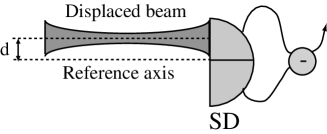
Figure 1: Split detection. The difference photo-current of the two halves measures the beam displacement, $d$.

At this stage we must introduce a more methodical representation of the beam. A beam of frequency $\omega$ can be represented by the positive frequency part of the electric field operator $\hat{\mathcal{E}}_{\rm in}^{+}e^{i\omega t}$. We are interested in the transverse information of the beam which is fully described by the slowly varying field envelope operator $\hat{\mathcal{E}}_{\rm in}^{+}$. We express this operator in terms of the displaced TEM_n0 basis modes, where $n$ denotes the order of the $x$-axis Hermite-Gauss mode. Since this paper considers one-dimensional beam displacement, we henceforth denote the beam amplitude function for the transverse modes with only one index. $\hat{\mathcal{E}}_{\rm in}^{+}$ can then be written as

$$\hat{\mathcal{E}}_{\rm in}^{+}=i\sqrt{\frac{\hbar\omega}{2\epsilon_{0}}}\sum_{n=0}^{\infty}\hat{a}_{n}u_{n}(x-d)$$ (6)

where $u_{n}(x-d)$ are the transverse beam amplitude functions for the displaced TEM_n0 modes and $\hat{a}_{n}$ are the corresponding annihilation operators. $\hat{a}_{n}$ is normally expressed as $\hat{a}_{n}=\alpha_{n}+\delta\hat{a}_{n}$, where $\alpha_{n}=\langle\hat{a}_{n}\rangle$ is the coherent amplitude and $\delta\hat{a}_{n}$ is a quantum noise operator. Since the beam is assumed to be a TEM₀₀ mode, only this mode has coherent excitation and therefore only $\alpha_{0}$ is nonzero. The field operator is then given by

$$\hat{\mathcal{E}}_{\rm in}^{+}=i\sqrt{\frac{\hbar\omega}{2\epsilon_{0}}}\left(\sqrt{N}u_{0}(x-d)+\sum_{n=0}^{\infty}\delta\hat{a}_{n}u_{n}(x-d)\right)$$ (7)

where $\alpha_{0}=\sqrt{N}$.

The difference photo-current, which provides information on the displacement of the beam relative to the centre of the detector, is given by

$$\hat{n}_{-} = \hat{n}_{x>0}-\hat{n}_{x<0}$$ (8)

$$= \frac{2\epsilon_{0}}{\hbar\omega}\left[\int_{-\infty}^{0}dx(\hat{\mathcal{E}}_{\rm in}^{+})^{\dagger}\hat{\mathcal{E}}_{\rm in}^{+}-\int_{0}^{\infty}dx(\hat{\mathcal{E}}_{\rm in}^{+})^{\dagger}\hat{\mathcal{E}}_{\rm in}^{+}\right]$$

where $\hat{n}_{x<0}$ and $\hat{n}_{x>0}$ are the photon number operators for the left and right halves of the detector, respectively. This expression can be simplified by changing bases from the TEM_n0 basis, to a TEM_n0 basis that has a $\pi$-phase flip at the center of the detector [13]. This new basis is defined by

$$v_{n}(x,d)=\left\{\begin{array}[]{ll}u_{n}(x)&\textrm{for }x>d\\ -u_{n}(x)&\textrm{for }x<d\end{array}\right.$$ (9)

and we denote annihilation operators for this basis as $\hat{b}_{n}$. If the incident TEM₀₀ field is bright, so that $N\gg|\langle\delta\hat{a}_{n}^{2}\rangle|$ for all $n$, the difference photo-current $\hat{n}_{-}$ can be written compactly as

$$\hat{n}_{-}=\sqrt{N}\left(\sqrt{N}\zeta_{0}+\delta\hat{Y}_{0}^{+}\right)$$ (10)

where $\hat{Y}_{0}^{+}$ is the amplitude quadrature operator associated with our new flipped basis, given by $\hat{Y}_{0}^{+}=\langle\hat{Y}_{0}^{+}\rangle+\delta\hat{Y}_{0}^{+}=\hat{b}_{0}+\hat{b}_{0}^{\dagger}$; and $\zeta_{0}(d)=\int_{-\infty}^{\infty}v_{0}(x,d)u_{0}(x-d)dx$ is the overlap coefficient between the first flipped mode and the TEM₀₀ mode. The beam displacement can be inferred from the mean photo-current

$$\langle\hat{n}_{-}\rangle=N\zeta_{0},$$ (11)

where the standard deviation of the photo-current noise is given by $\Delta\hat{n}_{-}=\sqrt{\langle\hat{n}_{-}^{2}\rangle-\langle\hat{n}_{-}\rangle^{2}}=\sqrt{N}\Delta\hat{Y}_{0}^{+}.$ For a coherent field, $\Delta\hat{Y}_{0}^{+}=1$, making $\Delta\hat{n}_{-}=\sqrt{N}$.

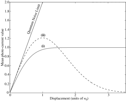
Figure 2: Mean value of the normalised difference photo-current, $\langle\hat{n}_{-}(d)\rangle/N$, as a function of beam displacement, $d$, for (i) split and (ii) TEM₁₀ homodyne detection.

Figure 2 (i) shows the normalised difference photo-current $\langle\hat{n}_{-}\rangle/N$ as a function of beam displacement, $d$, for split detection. We see that for small displacements where $d\ll w_{0}$, the normalised difference photo-current is linearly proportional to the displacement and can be approximated by

$$\langle\hat{n}_{-}\rangle_{d\ll w_{0}}=N\zeta_{0,d\ll w_{0}}\approx\sqrt{\frac{2}{\pi}}\frac{2Nd}{w_{0}}$$ (12)

As $d$ approaches the waist size of the beam, $w_{0}$, the normalised difference photo-current begins to roll off and asymptotes to a constant for larger $d$. This can be easily understood, since for $d\gg w_{0}$ the beam is incident almost entirely on one side of the detector. In this regime, large beam displacements only cause small variations in $\langle\hat{n}_{-}\rangle$, making is difficult to determine the beam displacement precisely.

The noise of our displacement measurement, $\Delta d_{\rm SD}$, is then related to the noise of the difference photo-current, $\Delta\hat{n}_{-}$, via

$$\Delta d_{\rm SD}=\frac{\partial d}{\partial\langle\hat{n}_{-}\rangle}\Delta\hat{n}_{-}$$ (13)

giving a sensitivity of

$${\cal S_{\rm SD}}=\frac{1}{\Delta d_{\rm SD}}=\frac{\partial\langle\hat{n}_{-}\rangle}{\partial d}\frac{1}{\sqrt{N}}=\frac{\partial\zeta_{0}}{\partial d}\sqrt{N}$$ (14)

for a coherent state. This sensitivity is plotted as a function of displacement in Figure 3 (i). In the region of small displacement, we have

$${\cal S}_{{\rm SD},d\ll w_{0}}\approx\sqrt{\frac{2}{\pi}}\frac{2\sqrt{N}}{w_{0}}$$ (15)

The efficiency of split detection for small displacement measurement is therefore given by the ratio

$$\epsilon_{\rm SD}=\frac{{\cal S}_{{\rm SD},d\ll w_{0}}}{{\cal S}_{\rm QNL}}=\sqrt{\frac{2}{\pi}}\sim 80\%$$ (16)

This $\sqrt{{2}/{\pi}}$ factor arises from the coefficient of the mode overlap integral, $\zeta_{0}$, between $v_{0}(x,d)$ and $u_{0}(x-d)$, as shown in Eq. (12). Fig. 3 (i) shows that the sensitivity of split detection decreases and asymptotes to zero for large displacement. The QNL in the figure confirms that split detection is not optimal for all displacement.

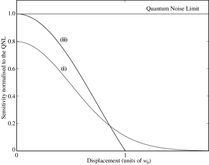
Figure 3: Sensitivity response of displacement measurement for (i) split and (ii) TEM₁₀ homodyne detection.

2.3 TEM₁₀ Homodyne Detection

Before proceeding with our proposal for an optimal small beam displacement measurement, let us express the displaced TEM₀₀ beam in terms of the centred Hermite-Gauss basis modes, $u_{n}(x)$. The coefficients of the decomposed basis modes are given by

$$\frac{\alpha_{n}}{\sqrt{N}}=\int_{-\infty}^{\infty}u_{0}(x-d)u_{n}(x)dx=\frac{d^{n}}{w_{0}^{n}\sqrt{n!}}\exp\left[-\frac{d^{2}}{2w_{0}^{2}}\right]$$ (17)

Plots of these coefficients as a function of beam displacement are shown in Fig. 4. We notice that for small displacement only the TEM₀₀ and TEM₁₀ modes have significant non-zero coefficients [9]. This means that the TEM₁₀ mode initially contributes most to the displacement signal. For larger displacement, other higher order modes become significant as their coefficients increase. This suggests that an interferometric measurement of the displaced beam with a centred TEM₁₀ mode may be optimal in the small displacement regime.

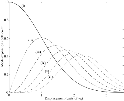
Figure 4: Coefficients of the decomposition of the displaced mode in terms of the TEM_n0 modes for the (i) TEM₀₀, (ii) TEM₁₀, (iii) TEM₂₀, (iv) TEM₃₀, (v) TEM₄₀ and (vi) TEM₅₀ mode components.

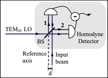
Figure 5: TEM₁₀ homodyne detection beam displacement measurement. BS: 50/50 beam-splitter, LO: local oscillator.

Figure 5 shows the TEM₁₀ detection scheme considered in this paper, the displaced beam is homodyned with a TEM₁₀ mode local oscillator. A reference axis for the displacement of the TEM₀₀ beam is defined by fixing the axis of the local oscillator. As can be seen from Fig. 4, when the input beam is centred, no power is contained in the TEM₁₀ mode. Due to the orthonomality of Hermite-Gauss modes, the TEM₁₀ local oscillator beam only detects the TEM₁₀ vacuum noise of the input beam. However we see from Fig. 4 that displacement of the TEM₀₀ input beam couples power into the (centred) TEM₁₀ mode. This coupled power interferes with the TEM₁₀ local oscillator, causing a change in the photo-current observed by the homodyne detector. Therefore, the homodyne detects a signal proportional to the displacement of the input beam.

The electric field operator describing the TEM₁₀ local oscillator beam is

$$\hat{\mathcal{E}}_{\rm LO}^{+}=\sqrt{\frac{\hbar\omega}{2\epsilon_{0}}}\left(\sqrt{N_{\rm LO}}u_{1}(x)+\sum_{n=0}^{\infty}\delta\hat{a}_{n}^{\rm LO}u_{n}(x)\right)$$ (18)

where the first bracketed term is the coherent amplitude, the second bracketed term denotes the quantum fluctuations of the beam, and $N_{\rm LO}$ is the number of photons in the local oscillator. Using this expression and that of the input displaced beam, the photon number operators corresponding to the two output beams of the beam-splitter are obtained, given by

$$\hat{n}_{1,2}=\frac{2\epsilon_{0}}{\hbar\omega}\int_{-\infty}^{\infty}(\hat{\mathcal{E}}^{+}_{1,2})^{\dagger}\hat{\mathcal{E}}^{+}_{1,2}dx$$ (19)

where subscripts $\{1,2\}$ denote the two output beams. From these, the difference photo-current between the two detectors used for homodyning is

$$\hat{n}_{-} = \sqrt{N_{\rm LO}}(2\alpha_{1}+\delta\hat{X}_{1}^{+})$$ (20)

$$= \sqrt{N_{\rm LO}}\left(\frac{2\sqrt{N}}{w_{0}}d+\delta\hat{X}_{1}^{+}\right)$$

where $\delta\hat{X}_{1}^{+}=\delta\hat{a}_{1}+\delta\hat{a}_{1}^{\dagger}$ is the amplitude quadrature noise operator of the TEM₁₀ component of the input beam, and we have assumed that $N_{\rm LO}\gg N$.

The mean photo-current as a function of beam displacement is shown in Figure 2 (ii). For small displacement, the mean photo-current is linearly proportional to the beam displacement. The factor of proportionality, $2\sqrt{N}/w_{0}$, in this case is the same as that of the array detection scheme. Hence, this shows that the measurement is optimal. In the large displacement regime, the photo-current decreases to zero. This is because the displacement signal couples to higher order modes.

The sensitivity response for the TEM₁₀ detection, obtained in the same manner as that for split detection, is shown in Figure 3 (ii). In the small displacement regime, we obtain

$${\cal S}_{H,d\ll w_{0}}=\frac{2\sqrt{N}}{w_{0}}$$ (21)

The efficiency of the TEM₁₀ detection is then

$$\epsilon_{H}=\frac{{\cal S}_{H,d\ll w_{0}}}{{\cal S}_{\rm QNL}}=100\%.$$ (22)

For larger displacement, the sensitivity decreases as the displacement increases. This is due to the power of the displaced beam being coupled to higher-ordered TEM_n0 modes (for $n>1$) and thus less power is contained in the TEM₁₀ mode.

3 Displacement measurement beyond the quantum noise limit

3.1 Split Detection with Squeezed Light

It has been shown that the noise measured by split detection is the flipped mode defined in Eq. (9) [13]. In order to improve the sensitivity of split detection, squeezing has to be introduced on the flipped mode. This method was demonstrated in the initial work of Treps et al. and the resulting spatial correlation between the two halves of the beam was termed spatial squeezing [10]. By applying a displacement modulation to the spatially squeezed beam, they demonstrated that sensitivities beyond the QNL could be achieved for beam displacement measurements. Treps et al. recently extended their one-dimensional spatial squeezing work to the two orthogonal transverse spatial axes [11, 12]. In this scenario, the photon correlation was measured between the set of top and bottom halves as well as left and right halves of a quadrant detector.

Restricting our analysis to one dimension, Fig. 6 (a) shows the combination of an input TEM₀₀ beam with a vacuum squeezed symmetric flipped mode $v(x,0)$ as defined in Eq. (9). Lossless combination of orthogonal spatial modes can be achieved in a number of ways. One example is the use of optical cavities for mixing resonant and non-resonant modes as illustrated by the Figure. The cavity reflects off the vacuum squeezed symmetric flipped mode whilst transmitting the TEM₀₀ beam. The total beam is then displaced and measured using a split-detector. The beam incident on the split detector is described by

$$\hat{\mathcal{E}}_{\rm in}^{+} = i\sqrt{\frac{\hbar\omega}{2\epsilon_{0}}}\Big{(}\sqrt{N}u_{0}(x-d)+\delta\hat{c}_{0}^{\rm sqz}v_{0}(x-d,0)$$ (23)

$$+\sum_{n=1}^{\infty}\delta\hat{c}_{n}v_{n}(x-d,0)\Big{)}$$

where the first term arises from the TEM₀₀ mode while the second term describes the vacuum squeezed flipped mode and the last term in Eq. (23) represents all other higher order vacuum noise terms. The photo-current difference operator in the limit of small displacement is

$$\hat{n}_{-}=\sqrt{N}\left(\sqrt{\frac{2}{\pi}}\frac{2\sqrt{N}}{w_{0}}d+\delta\hat{Z}_{0,{\rm sqz}}^{+}\xi_{0}+\sum_{n=1}^{\infty}\delta\hat{Z}_{n}^{+}\xi_{n}\right)$$ (24)

where $\delta\hat{Z}_{n}^{+}=\delta\hat{c}_{n}+\delta\hat{c}_{n}^{\dagger}$ are the amplitude quadrature operators. The first bracketed term arises from the mode overlap between the $v_{0}(x,0)$ and $u_{0}(x-d)$ modes, which has a value of $\sqrt{2/\pi}$. The second term originates from the mode overlap between the $v_{0}(x,d)$ and $v_{0}(x-d,0)$ modes. The last term is a result of the overlap between the $v_{0}(x,d)$ and $v_{n}(x-d,0)$ modes. The overlap coefficients are given by $\xi_{n}=\int_{-\infty}^{\infty}v_{0}(x,d)v_{n}(x-d,0)dx$.

Figure 7 (i) plots the sensitivity, $\cal{S}_{\rm SD}$, as a function of squeezing. Notice that the QNL can only be surpassed with more than 1.9 dB of squeezing. This is a direct consequence of the intrinsic inefficiency of displacement measurement using split detection.

3.2 TEM₁₀ Homodyne Detection with Squeezed Light

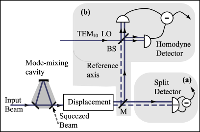
Figure 6: Measurement options: (a) Split detection with a vacuum squeezed symmetric flipped mode or (b) TEM₁₀ homodyne detection with a vacuum squeezed TEM₁₀ mode. Both schemes combine the squeezed beam and the TEM₀₀ input beam losslessly using an optical cavity. M: mirror, BS: 50/50 beam-splitter, LO: local oscillator.

We have shown that by squeezing the flipped mode and detecting the beam displacement using a split detector, one is able to improve on the displacement sensitivity to beyond the QNL. Correspondingly, we now consider the effect of squeezing the TEM₁₀ mode in our homodyne detection. Figure 6 shows the combination of the TEM₀₀ input beam with a vacuum squeezed TEM₁₀ beam prior to displacement. The displaced beam is then analysed using homodyne detection with a TEM₁₀ local oscillator beam as discussed previously (see Fig. 6 (b)). The detected beam is given by

$$\hat{\mathcal{E}}_{\rm in}^{+} = i\sqrt{\frac{\hbar\omega}{2\epsilon_{0}}}\Big{(}\sqrt{N}u_{0}(x-d)+\delta\hat{a}_{1}^{\rm sqz}u_{1}(x-d)$$ (25)

$$+\sum_{n\neq 1}^{\infty}\delta\hat{a}_{n}u_{n}(x-d)\Big{)}$$

where the first term arises from the TEM₀₀ mode, the second term from the squeezed vacuum TEM₁₀ mode, and the last term from higher ordered vacuum noise. The difference photo-current between the two detectors used for homodyning is given by

$$\hat{n}_{-}=\sqrt{N_{LO}}\Big{(}\frac{2\sqrt{N}}{w_{0}}d+\delta\hat{X}_{1,{\rm sqz}}^{+}\chi_{1}+\sum_{n\neq 1}^{\infty}\delta\hat{X}_{n}^{+}\chi_{n}\Big{)}$$ (26)

where $\chi_{n}=\int_{-\infty}^{\infty}u_{1}(x)u_{n}(x-d)dx$. For small displacement, the overlap between the vacuum squeezed mode and the local oscillator beam is $\sim 100\%$ whilst the last term is negligible.

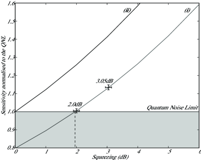
Figure 7: Plots of sensitivity, $\cal{S}$, for small displacement, as a function of squeezing for (i) split and (ii) TEM₁₀ homodyne detection. Shading indicates the region where displacement measurement is below the QNL. The data points were obtained from Ref. [11].

The sensitivity, $\cal{S}_{H}$, as a function of squeezing on the TEM₁₀ mode is shown in Fig. 7 (ii). Since the scheme is optimum for small displacement, any amount of squeezing will lead to a sensitivity beyond the QNL. Furthermore, the TEM₁₀ detection surpasses the performance of split detection for all values of squeezing.

3.3 Discussion

In the paper on quantum displacement measurement by Treps et al. [11], displacement measurements of the two transverse axes were performed using split detection with two co-propagating squeezed beams. The squeezing values were 2.0 dB and 3.05 dB for the vertical and horizontal displacement measurement, respectively. Relating this result back to our analysis, we find that the displacement measurements performed were indeed beyond the QNL. These corresponded to sensitivities of 100.5% and 113.0% above the QNL as shown in Fig. 7. However, using the same squeezed beams but adopting the TEM₁₀ homodyne detection, sensitivities of 126% and 141.5% above the QNL would be achievable.

The TEM₁₀ homodyne detection can be extended to perform beam displacement measurements in both transverse dimensions. The TEM₁₀ mode component is responsible for beam displacement in one transverse axis. Thus, by symmetry, the TEM₀₁ mode component is responsible for beam displacement in the orthogonal transverse axis. Correspondingly, beam displacement measurement in the horizontal or vertical transverse axis can be achieved by adapting the mode-shape of the local oscillator beam to either TEM₁₀ or TEM₀₁. To perform optimum larger beam displacement measurements, the local oscillator of the TEM₁₀ homodyne detection can be modified by including higher order components of the TEM₀₀ displaced beam. Similarly, the homodyning scheme can be extended to measuring displacements of arbitrary mode-shapes assuming a priori knowledge of the beam shape.

4 Conclusion

By defining the beam position as the mean photon position of a light beam, optical beam displacement can be measured with reference to a fixed axis. Using an idealised array detection scheme, we derived the QNL associated with optical displacement measurements. A displaced TEM₀₀ beam can be decomposed into an infinite series of Hermite-Gauss modes but in the limit of small displacement, only the TEM₀₀ and TEM₁₀ components are non-negligible. Since the split detector effectively measures the noise of an optical flipped mode [13], it is only $\sim 80\%$ efficient when used to measure the displacement of a TEM₀₀ beam. We have proposed an optimum displacement measurement scheme based on homodyne detection. By using a TEM₁₀ local oscillator, small displacement signals can be extracted with 100% efficiency. We showed that in this small displacement regime the TEM₁₀ homodyne detection performs at the QNL, and is significantly more efficient than split detection.

We have also shown that by mixing the input beam with a squeezed beam in the appropriate mode, we can significantly improve the sensitivity of the TEM₁₀ homodyne detection. We compared the sensitivities of both split and TEM₁₀ homodyne detection for equal values of squeezing and found that for small displacements the TEM₁₀ detection outperforms split detection for all values of squeezing. For split detection, more than 1.9 dB of squeezing is required to achieve a sensitivity beyond the QNL. Whilst for the TEM₁₀ detection any amount of squeezing will suffice.

5 Acknowledgment

We thank Nicolai Grosse and Nicolas Treps for fruitful discussions. This work is funded by the Australian Research Council Centre of Excellence Program.

References

- [1] T. Santhanakrishnan, N. Krishna Mohan, M. D. Kothiyal and R. S. Sirohi, J. Opt., 24, 109 (1995).
- [2] C. A. Putman, B. G. De Grooth, N. F. Van Hulst and J. Greve, J. Appl. Phys., 72, 6 (1992).
- [3] S. Arnon, Appl. Opt., 37, 5031 (1998).
- [4] V. V. Nikulin, M. Bouzoubaa, V. A. Skormin and T. E. Busch, Opt. Eng., 40, 2208 (2001).
- [5] H.-L. Guo, C.-X. Liu, Z.-L. Li, J.-F. Duan, X.-H. Han, B.-Y. Chen and D.-Z. Zhang, Chinese Phys. Lett., 20, 950 (2003).
- [6] R. M. Simmons, J. T. Finer, S. Chu and J. A. Spudich, Biophys. J., 70, 1813 (1996).
- [7] F. Gittes and C. F. Schmidt, Opt. Lett., 23, 7 (1998).
- [8] W. Denk and W. W. Webb, Appl. Opt., 29, 2382 (1990).
- [9] D. Z. Anderson, Appl. Opt., 23, 2944 (1984).
- [10] N. Treps, U. Andersen, B. C. Buchler, P. K. Lam, A. Maître, H.-A. Bachor and C. Fabre, Phys. Rev. Lett., 88, 203601 (2002).
- [11] N. Treps, N. Grosse, W. P. Bowen, C. Fabre, H.-A. Bachor and P. K. Lam, Science, 301, 940 (2003).
- [12] N. Treps, N. Grosse, W. P. Bowen, M. T. L. Hsu, A. Maître, C. Fabre, H.-A. Bachor and P. K. Lam, J. Opt. B (in print); preprint : quant-ph/0311122.
- [13] C. Fabre, J. B. Fouet and A. Maître, Opt. Lett., 76, 76 (2000).
- [14] V. Delaubert, D. A. Shaddock, P. K. Lam, B. C. Buchler, H.-A. Bachor and D. E. McClelland, J. Opt. A, 4, 393 (2002).