Distinguishing between optical coherent states with imperfect detection

Abstract

Several proposed techniques for distinguishing between optical coherent states are analyzed under a physically realistic model of photodetection. Quantum error probabilities are derived for the Kennedy receiver, the Dolinar receiver and the unitary rotation scheme proposed by Sasaki and Hirota for sub-unity detector efficiency. Monte carlo simulations are performed to assess the effects of detector dark counts, dead time, signal processing bandwidth and phase noise in the communication channel. The feedback strategy employed by the Dolinar receiver is found to achieve the Helstrom bound for sub-unity detection efficiency and to provide robustness to these other detector imperfections making it more attractive for laboratory implementation than previously believed.

I Introduction

Communication is subject to quantum mechanical indeterminism even when the transmitted information is entirely classical. This potentially counter-intuitive property results from the fact that information must be conveyed through a physical medium— a communication channel— that is unavoidably governed by quantum mechanics. From this perspective, the sender encodes information by preparing the channel into a well-defined quantum state, $\hat{\rho}$, selected from a predetermined alphabet, $\mathcal{A}\equiv\{\hat{\rho}_{0},\ldots,\hat{\rho}_{M}\}$, of codewords. The receiver, following any relevant signal propagation, performs a measurement on the channel to ascertain which state was transmitted by the sender.

A quantum mechanical complication arises when the states in $\mathcal{A}$ are not orthogonal, as no measurement can distinguish between overlapping quantum states without some ambiguity von Neumann (1955); Holevo (1973); Helstrom (1976); Fuchs and Peres (1996). This uncertainty in determining the channel state translates into a non-zero probability that the receiver will misinterpret the transmitted codeword and produce a communication error. While it would seem obvious that the sender should simply adopt an alphabet of orthogonal states, it is rarely practicable to communicate under such ideal conditions Yuen and Shapiro (1978); Usuda and Hirota (1995). Even when it is possible for the sender to transmit orthogonal codewords, inevitable imperfections in the channel including decoherence and energy dissipation quickly damage that orthogonality. In some cases, the classical information capacity of a noisy channel is actually maximized by a nonorthogonal alphabet Fuchs (1997).

When developing a communication system to operate at the highest feasible rate given fixed channel properties and a constrained capability for state preparation, the objective is to minimize the communication error by designing a “good” receiver. Distinguishing between nonorthogonal states is a pervasive problem in quantum information theory Peres and Wootters (1991); Fuchs (1996) addressed mathematically by optimizing a state-determining measurement over all positive operator valued measures (POVMs) Davies and Lewis (1970); Helstrom (1976); Kraus (1983). This general approach can be applied to communication; however, arbitrary POVMs are rarely straightforward to implement in the laboratory. Therefore, a “good” receiver must balance quantum mechanical optimality with implementability and robust performance under realistic experimental conditions.

For example, the optical field produced by a laser provides a convenient quantum system for carrying information. Of course, optical coherent states are not orthogonal and cannot be distinguished perfectly by photodetection. While the overlap between different coherent states can be reduced by employing large amplitudes, power limitations often restrict $\mathcal{A}$ to the small-amplitude regime where quantum effects dominate. This is especially true in situations (such as optical fibers) where the communication medium behaves nonlinearly at high power, as well as for long distance communication where signals are substantially attenuated, including deep space transmission.

Motivated by these experimental considerations, optimizing a communication process based on small-amplitude optical coherent states and photodetection has been an active subject since the advent of the laser Kennedy (1972); Dolinar (1973); Usuda and Hirota (1995); Belavkin et al. (1995). Kennedy initially proposed a receiver based on simple photon counting to distinguish between two different coherent states Kennedy (1972). However, the Kennedy receiver error probability lies above the quantum mechanical minimum Helstrom (1976) (or Helstrom bound) and this prompted Dolinar to devise a measurement scheme capable of achieving the quantum limit Dolinar (1973). Dolinar’s receiver, while still based on photon counting, approximates an optimal POVM by adding a local feedback signal to the channel; but, this procedure has often been deemed impractical Monmose et al. (1996) due to the need for real-time adjustment of the local signal following each photon arrival. As a result, Sasaki and Hirota later proposed an alternative receiver that applies an open-loop unitary transformation to the incoming coherent state signals to render them more distinguishable by simple photon counting Usuda and Hirota (1995); Monmose et al. (1996); Sasaki and Hirota (1996) .

However, recent experimental advances in real-time quantum-limited feedback control Armen et al. (2002); Geremia et al. (2004); JM GEremia and Mabuchi (2004) suggest that the Dolinar receiver may be more experimentally practical than previously believed. The opinion that feedback should be avoided in designing an optical receiver is grounded in the now-antiquated premise that real-time adaptive quantum measurements are technologically inaccessible. Most arguments in favor of passive devices have been based on idealized receiver models that assume, for example, perfect photon counting efficiency. A fair comparison between open and closed-loop receivers should take detection error into account— feedback generally increases the robustness of the measurement device in exchange for the added complexity.

Here, we consider the relative performance of the Kennedy, Dolinar and Sasaki-Hirota receivers under realistic experimental conditions that include: (1) sub-unity quantum efficiency, where it is possible for the detector miscount incoming photons, (2) non-zero dark-counts, where the detector can register photons even in the absence of a signal, (3) non-zero dead-time, or finite detector recovery time after registering a photon arrival, (4) finite bandwidth of any signal processing necessary to implement the detector, and (5) fluctuations in the phase of the incoming optical signal.

II Binary Coherent State Communication

An optical binary communication protocol can be implemented via the alphabet consisting of two pure coherent states, $\hat{\rho}_{0}=|\Psi_{0}\rangle\langle\Psi_{0}|$, and $\hat{\rho}_{1}=|\Psi_{1}\rangle\langle\Psi_{1}|$. Without loss of generality, we will assume that logical 0 is represented by the vacuum,

$$\Psi_{0}(t)=0\,,$$ (1)

and that logical 1 is represented by

$$\Psi_{1}(t)=\psi_{1}(t)\exp\left[-i(\omega t+\varphi)\right]+\mathrm{c.c.},$$ (2)

where $\omega$ is the frequency of the optical carrier and $\varphi$ is (ideally) a fixed phase. The envelope function, $\psi_{1}(t)$, is normalized such that

$$\int_{0}^{T}|\psi_{1}(t)|^{2}\,dt=\bar{N}\,,$$ (3)

where $\bar{N}$ is the mean number of photons to arrive at the receiver during the measurement interval, $0\leq t\leq T$. That is, $\hbar\omega|\psi_{1}(t)|^{2}$ is the instantaneous average power of the optical signal for logical 1.

This alphabet, $\mathcal{A}=\{\hat{\rho}_{0},\hat{\rho}_{1}\}$, is applicable to both amplitude and phase-shift keyed communication protocols as it is always possible to transform between the two by combining the incoming signal with an appropriate local oscillator. That is, amplitude keying with $\mathcal{A}=\{|0\rangle,|\alpha\rangle\}$ (for some coherent state $|\alpha\rangle$ with amplitude, $\alpha$) is equivalent to the phase-shift keyed alphabet, $\{|-\frac{1}{2}\alpha\rangle,|\frac{1}{2}\alpha\rangle\}$, via a displacement, $\hat{D}\left[-\frac{1}{2}\alpha\right]\equiv\exp(-\frac{1}{2}(\alpha\hat{a}^{\dagger}-\alpha^{*}\hat{a}))$, where $\hat{a}^{\dagger}$ and $\hat{a}$ are the creation and annihilation operators for the channel mode. Similarly, if $|\Psi_{0}\rangle\neq|0\rangle$, a simple displacement can be used restore $|\Psi_{0}\rangle$ to the vacuum state.

II.1 The Quantum Error Probaility

The coherent states, $\hat{\rho}_{0}$ and $\hat{\rho}_{1}$, are not orthogonal, so it is impossible for a receiver to identify the transmitted state without sometimes making a mistake. That is, the receiver attempts to ascertain which state was transmitted by performing a quantum measurement, $\Upsilon$, on the channel. $\Upsilon$ is described by an appropriate POVM represented by a complete set of positive operators Peres (1990),

$$\sum_{n}\hat{\Upsilon}_{n}=\hat{\mathbbm{1}}\,\quad\hat{\Upsilon}_{n}\geq 0\,,$$ (4)

where $n$ indexes the possible measurement outcomes. For binary communication, it is always possible (and optimal) for the receiver to implement the measurement as a decision between two hypotheses: $(H_{0})$, that the transmitted state is $\hat{\rho}_{0}$, selected when the measurement outcome corresponds to $\hat{\Upsilon}_{0}$, and $(H_{1})$, that the transmitted state is $\hat{\rho}_{1}$, selected when the measurement outcome corresponds to $\hat{\Upsilon}_{1}$.

Given the positive operators, $\hat{\Upsilon}_{0}+\hat{\Upsilon}_{1}=\hat{\mathbbm{1}}$, there is some chance that the receiver will select the null hypothesis, $H_{0}$, when $\hat{\rho}_{1}$ is actually present,

$$p(H_{0}|\hat{\rho}_{1})=\mathrm{tr}[\hat{\Upsilon}_{0}\hat{\rho}_{1}]=\mathrm{tr}[(\hat{\mathbbm{1}}-\hat{\Upsilon}_{1})\hat{\rho}_{1}]\,.$$ (5)

And, it will sometimes select $H_{1}$ when $\hat{\rho}_{0}$ is present,

$$p(H_{1}|\hat{\rho}_{0})=\mathrm{tr}[\hat{\Upsilon}_{1}\hat{\rho}_{0}]\,.$$ (6)

The total receiver error probability depends upon the choice of $\hat{\Upsilon}_{0}$ and $\hat{\Upsilon}_{1}$ and is given by

$$p[\hat{\Upsilon}_{0},\hat{\Upsilon}_{1}]=\xi_{0}p(H_{1}|\hat{\rho}_{0})+\xi_{1}p(H_{0}|\hat{\rho}_{1})\,.$$ (7)

Here, $\xi_{0}=p_{0}(\hat{\rho}_{0})$ and $\xi_{1}=p_{0}(\hat{\rho}_{1})$ are the probabilities that the sender will transmit $\hat{\rho}_{0}$ and $\hat{\rho}_{1}$ respectively; they reflect the prior knowledge that enters into the hypothesis testing process implemented by the receiver, and in many cases $\xi_{0}=\xi_{1}=1/2$.

Minimizing the receiver measurement over POVMs (over $\hat{\Upsilon}_{0}$ and $\hat{\Upsilon}_{1}$) leads to a quantity known as the quantum error probability,

$$P_{\mathrm{H}}\equiv\min_{\hat{\Upsilon}_{0},\hat{\Upsilon}_{1}}p[\hat{\Upsilon}_{0},\hat{\Upsilon}_{1}]\,,$$ (8)

also referred to as the Helstrom bound. $P_{\mathrm{H}}$ is the smallest physically allowable error probability, given the overlap between $\hat{\rho}_{0}$ and $\hat{\rho}_{1}$.

II.1.1 The Helstrom Bound

Helstrom demonstrated that minimizing the receiver error probability,

$$p[\hat{\Upsilon}_{0},\hat{\Upsilon}_{1}] = \xi_{0}\mathrm{tr}\left[\hat{\Upsilon}_{1}\hat{\rho}_{0}\right]+\xi_{1}\mathrm{tr}\left[(\hat{\mathbbm{1}}-\hat{\Upsilon}_{1})\hat{\rho}_{1}\right]$$ (9)

$$= \xi_{1}+\mathrm{tr}\left[\hat{\Upsilon}_{1}(\xi_{0}\hat{\rho}_{0}-\xi_{1}\hat{\rho}_{1})\right]$$ (10)

is accomplished by optimizing

$$\min_{\hat{\Upsilon}_{1}}\mathrm{tr}[\hat{\Upsilon}_{1}\hat{\Gamma}]\,,\quad\hat{\Gamma}=\xi_{0}\hat{\rho}_{0}-\xi_{1}\hat{\rho}_{1}$$ (11)

over $\hat{\Upsilon}_{1}$ subject to $0\leq\hat{\Upsilon}_{1}\leq\hat{\mathbbm{1}}$ Helstrom (1976). Given the spectral decomposition,

$$\hat{\Gamma}=\sum_{n}\lambda_{n}|n\rangle\langle n|\,$$ (12)

where the $\lambda_{n}$ are the eigenvalues of $\hat{\Gamma}$, the resulting Helstrom bound can be expressed as Helstrom (1967)

$$P_{\mathrm{H}}=\xi_{1}+\sum_{\lambda_{n}<0}\lambda_{n}\,.$$ (13)

For pure states, where $\hat{\rho}_{0}=|\Psi_{0}\rangle\langle\Psi_{0}|$ and $\hat{\rho}_{1}=|\Psi_{1}\rangle\langle\Psi_{1}|$, $\hat{\Gamma}$ has two eigenvalues of which only one is negative,

$$\lambda_{-}=\frac{1}{2}\left(1-\sqrt{1-4\xi_{0}\xi_{1}|\langle\Psi_{0}|\Psi_{1}\rangle|^{2}}\right)-\xi_{1}>0\,,$$ (14)

and the quantum error probability is therefore Helstrom (1976)

$$P_{\mathrm{H}}=\frac{1}{2}\left(1-\sqrt{1-4\xi_{0}\xi_{1}|\langle\Psi_{1}|\Psi_{0}\rangle|^{2}}\right)\,.$$ (15)

The Helstrom bound is readily evaluated for coherent states by employing the relation Glauber (1963),

$$|\alpha\rangle=e^{-|\alpha|^{2}/2}\sum_{n=0}^{\infty}\frac{\alpha^{n}}{\sqrt{n!}}|n\rangle\,,$$ (16)

to compute the overlap between $|\Psi_{1}\rangle$ and $|\Psi_{0}\rangle$,

$$c_{0}\equiv\langle\Psi_{1}|\Psi_{0}\rangle=e^{-\bar{N}/2}\,.$$ (17)

It is further possible to evaluate the Helstrom bound for imperfect detection. Coherent states have the convenient property that sub-unity quantum efficiency is equivalent to an ideal detector masked by a beam-splitter with transmission coefficient, $\eta\leq 1$, to give

$$P_{\mathrm{H}}(\eta)=\frac{1}{2}\left(1-\sqrt{1-4\xi_{0}\xi_{1}c_{0}^{2\eta}}\right)\,.$$ (18)

This result and Eq. (15) indicate that there is a finite quantum error probability for all choices of $|\Psi_{1}\rangle$, even when an optimal measurement is performed.

II.2 The Kennedy Receiver

Kennedy proposed a near-optimal receiver that simply counts the number of photon arrivals registered by the detector between $t=0$ and $T$. It decides in favor of $H_{0}$ when the number of clicks is zero, otherwise $H_{1}$ is chosen. This hypothesis testing procedure corresponds to the measurement operators,

$$\hat{\Upsilon}_{0} = |0\rangle\langle 0|$$ (19)

$$\hat{\Upsilon}_{1} = \sum_{n=1}^{\infty}|n\rangle\langle n|\,$$ (20)

where $|n\rangle$ are the eigenvectors of the number operator, $\hat{N}=\hat{a}^{\dagger}\hat{a}$.

The Kennedy receiver has the property that it always correctly selects $H_{0}$ when the channel is in $\hat{\rho}_{0}$, since the photon counter will never register photons when the vacuum state is present (ignoring background light and detector dark-counts for now). Therefore, $p(H_{1}|\hat{\rho}_{0})=0$, however,

$$p(H_{0}|\hat{\rho}_{1})\equiv\mathrm{tr}[\hat{\Upsilon}_{0}\hat{\rho}_{1}]=|\langle 0|\Psi_{1}\rangle|^{2}$$ (21)

is non-zero due to the finite overlap of all coherent states with the vacuum. The Poisson statistics of coherent state photon numbers allows for the possibility that zero photons will be recorded even when $\hat{\rho}_{1}$ is present.

Furthermore, an imperfect detector can misdiagnose $\hat{\rho}_{1}$ if it fails to generate clicks for photons that do arrive at the detector. The probability for successfully choosing $H_{1}$ when $\hat{\rho}_{1}$ is present is given by,

$$p_{\eta}(H_{1}|\hat{\rho}_{1})=\sum_{n=1}^{\infty}\sum_{k=1}^{\infty}p(n,k)|\langle n|\alpha\rangle|^{2}$$ (22)

where the Bernoulli distribution,

$$p(n,k)=\frac{n!}{k!(n-k)!}\eta^{k}(1-\eta)^{n-k}$$ (23)

gives the probability that a detector with quantum efficiency, $\eta$, will register $k$ clicks when the actual number of photons is $n$. The resulting Kennedy receiver error,

$$P_{\mathrm{K}}(\eta)=1-p_{\eta}(H_{1}|\hat{\rho}_{1})=\xi_{1}c_{0}^{2\eta}\,.$$ (24)

asymptotically approaches the Helstrom bound for large signal amplitudes, but is larger for small photon numbers.

II.3 The Sasaki-Hirota Receiver

Sasaki and Hirota proposed that it would be possible to achieve the Helstrom bound using simple photon counting by applying a unitary transformation to the incoming signal states prior to detection Usuda and Hirota (1995); Monmose et al. (1996); Sasaki and Hirota (1996). They considered rotations,

$$\hat{U}[\theta]=\exp\left[\theta(|\Psi_{0}^{\prime}\rangle\langle\Psi_{1}^{\prime}|-|\Psi_{1}^{\prime}\rangle\langle\Psi_{0}^{\prime}|)\right]\,,$$ (25)

F generated by the transformed alphabet, $\mathcal{A}^{\prime}$,

$$|\Psi_{0}^{\prime}\rangle=|\Psi_{0}\rangle,\quad|\Psi_{1}^{\prime}\rangle=\frac{|\Psi_{1}\rangle-c_{0}|\Psi_{0}\rangle}{\sqrt{1-c_{0}^{2}}}\,,$$ (26)

obtained from Gram-Schmidt orthogalization of $\mathcal{A}$. The rotation angle, $\theta\in\mathbbm{R}$, is a parameter that must be optimized in order to achieve the Helstrom bound.

Application of $\hat{U}[\theta]$ on the incoming signal states (which belong to the original alphabet, $\mathcal{A}$) leads to the transformed states,

$$\hat{U}[\theta]|\Psi_{0}\rangle = \left(\cos\theta+\frac{c_{0}\sin\gamma}{\sqrt{1-c_{0}^{2}}}\right)|\Psi_{0}\rangle$$ (27)

$$-\frac{\sin\theta}{\sqrt{1-c_{0}^{2}}}|\Psi_{1}\rangle$$

and

$$\hat{U}[\theta]|\Psi_{1}\rangle = \frac{\sin\theta}{\sqrt{1-c_{0}^{2}}}|\Psi_{0}\rangle$$

$$+\frac{\cos\theta\sqrt{1-c_{0}^{2}}-c_{0}\sin\theta}{\sqrt{1-c_{0}^{2}}}|\Psi_{1}\rangle\,.$$

Since $|\Psi_{0}^{\prime}\rangle$ is the vacuum state, hypothesis testing can still be performed by simple photon counting. However, unlike the Kennedy receiver, it is possible to misdiagnose $\hat{\rho}_{0}$ since $\hat{U}[\theta]|\Psi_{0}\rangle$ contains a non-zero contribution from $|\Psi_{1}\rangle$. The probability for a false-positive detection by a photon counter with efficiency, $\eta$, is given by

$$p_{\eta}^{\theta}(H_{1}|\hat{\rho}_{0}) = \sum_{n=1}^{\infty}\sum_{k=1}^{\infty}p(n,k)|\langle n|\hat{U}[\theta]|\Psi_{0}\rangle|^{2}$$ (29)

$$= \frac{c_{0}^{2\eta}-1}{c_{0}^{2}-1}\sin^{2}\theta$$ (30)

which is evaluated by recognizing that

$$\langle n|\hat{U}[\theta]|\Psi_{0}\rangle = \left[\cos\theta+\frac{c_{0}\sin\theta}{\sqrt{1-c_{0}^{2}}}\right]\delta_{n,0}$$ (31)

$$-\frac{c_{0}\alpha^{n}\sin\theta}{\sqrt{n!(1-c_{0}^{2})}}\,,$$

where $\alpha$ is the (complex) amplitude of $|\Psi_{1}\rangle$. The probability for correct detection can be similarly obtained to give

$$p_{\eta}^{\theta}(H_{1}|\hat{\rho}_{1}) = \sum_{n=1}^{\infty}\sum_{k=1}^{\infty}p(n,k)|\langle n|\hat{U}[\theta]|\Psi_{1}\rangle$$ (32)

$$= \frac{c_{0}^{2\eta}-1}{c_{0}^{2}-1}\left[c_{0}\sin\theta-\sqrt{1-c_{0}^{2}}\cos\theta\right]^{2}$$ (33)

by employing the relationship,

$$\langle n|\hat{U}[\theta]|\Psi_{1}\rangle = \left[c_{0}\cos\theta-\frac{c_{0}^{2}\alpha^{n}\sin\theta}{\sqrt{n!(1-c_{0}^{2})}}\right]$$ (34)

$$+\frac{\sin\theta}{\sqrt{1-c_{0}^{2}}}\delta_{n,0}\,.$$

The total Sasaki-Hirota receiver error is given by the weighted sum,

$$P_{\mathrm{SH}}(\eta,\theta)=\xi_{0}p_{\eta}^{\theta}(H_{1}|\hat{\rho}_{0})+\xi_{1}\left[1-p_{\eta}^{\theta}(H_{1}|\hat{\rho}_{1})\right]$$ (35)

and can be minimized over $\theta\in\mathbbm{R}$ to give

$$\theta=-\tan^{-1}\sqrt{\frac{\sqrt{1-4\xi_{0}\xi_{1}c_{0}^{2}}-1+2\xi_{1}c_{0}^{2}}{\sqrt{1-4\xi_{0}\xi_{1}c_{0}^{2}}+1-2\xi_{1}c_{0}^{2}}}\,.$$ (36)

For perfect detection efficiency, $\eta=1$, Eq. (35) is equivalent to the Helstrom bound; however, for $\eta<1$, it is larger.

II.4 The Dolinar Receiver

The Dolinar receiver takes a different approach to achieving the Helstrom bound with a photon counting detector; it utilizes an adaptive strategy to implement a feedback approximation to the Helstrom POVM Dolinar (1973, 1976). Dolinar’s receiver operates by combining the incoming signal, $\Psi(t)$, with a separate local signal,

$$U(t)=u(t)\exp\left[-i(\omega t+\phi)\right]+\mathrm{c.c}\,,$$ (37)

such that the detector counts photons with total instantaneous mean rate,

$$\Phi(t)=|\psi(t)+u(t)|^{2}\,.$$ (38)

Here, $\psi(t)=0$ when the channel is in the state $\hat{\rho}_{0}$, and $\psi(t)=\psi_{1}(t)$ when the channel is in $\hat{\rho}_{1}$ [refer to Eqs. (1) and (2)].

The receiver decides between hypotheses $H_{0}$ and $H_{1}$ by selecting the one that is more consistent with the record of photon arrival times observed by the detector given the choice of $u(t)$. $H_{1}$ is selected when the ratio of conditional arrival time probabilities,

$$\Lambda=\frac{p_{\eta}\left[\hat{\rho}_{1}|t_{1},\ldots,t_{n},u(t)\right]}{p_{\eta}\left[\hat{\rho}_{0}|t_{1},\ldots,t_{n},u(t)\right]}\,,$$ (39)

is greater than one; otherwise it is assumed that $\hat{\rho}_{0}$ was transmitted. The conditional probabilities, $p_{\eta}\left[\hat{\rho}_{i}|t_{1},\ldots,t_{n},u(t)\right]$, reflect the likelihood that $n$ photon arrivals occur precisely at the times, $\{t_{1},\ldots,t_{n}\}$, given that: the channel is in the state, $\hat{\rho}_{i}$, the feedback amplitude is $u(t)$, and the detector quantum efficiency is $\eta$.

We see that this decision criterion based on $\Lambda$ is immediately related to the error probabilities,

$$\Lambda=\frac{p_{\eta}\left[H_{1}|\hat{\rho}_{1},u(t)\right]}{p_{\eta}\left[H_{1}\hat{\rho}_{0},u(t)\right]}=\frac{1-p_{\eta}\left[H_{0}|\hat{\rho}_{1},u(t)\right]}{p_{\eta}\left[H_{1}|\hat{\rho}_{0},u(t)\right]},$$ (40)

when $\Lambda>1$ (i.e., the receiver definitely selects $H_{1}$), and

$$\Lambda=\frac{p_{\eta}\left[H_{0}|\hat{\rho}_{1},u(t)\right]}{p_{\eta}\left[H_{0}|\hat{\rho}_{0},u(t)\right]}=\frac{p_{\eta}\left[H_{0}|\hat{\rho}_{1},u(t)\right]}{1-p_{\eta}\left[H_{1}|\hat{\rho}_{0},u(t)\right]}$$ (41)

when $\Lambda<1$ (i.e., the receiver definitely selects $H_{0}$). Similarly, the likelihood ratio, $\Lambda$, can be reëxpressed in terms of the photon counting distributions frequently encountered in quantum optics by employing Bayes’ rule,

$$\Lambda = \frac{p_{\eta}\left[t_{1},\ldots,t_{n}|\hat{\rho}_{1},u(t)\right]p_{0}(\hat{\rho}_{1})}{p_{\eta}\left[t_{1},\ldots,t_{n}|\hat{\rho}_{0},u(t)\right]p_{0}(\hat{\rho}_{0})}$$ (42)

$$= \frac{\xi_{1}}{\xi_{0}}\frac{p_{\eta}\left[t_{1},\ldots,t_{n}|\hat{\rho}_{1},u(t)\right]}{p_{\eta}\left[t_{1},\ldots,t_{n}|\hat{\rho}_{0},u(t)\right]}\,,$$ (43)

where the $p_{\eta}\left[t_{1},\ldots,t_{n}|\hat{\rho}_{i},u(t)\right]$ are the exclusive counting densities,

$$p_{\eta}\left[t_{1},\ldots,t_{n}|\hat{\rho}_{i},u(t)\right]=\prod_{k=1}^{n+1}w_{\eta}\left[t_{k}|\hat{\rho}_{i},u(t)\right]\,.$$ (44)

Here, $t_{0}=0$, $t_{n+1}=T$, and $w_{\eta}\left[t_{k}|\hat{\rho}_{i},u(t)\right]$ is the exponential waiting time distribution,

$$w\left[t_{k}|\hat{\rho}_{i},u(t)\right]=\eta\Phi(t_{k})\,\exp\left(-\eta\int_{t_{k-1}}^{k}\Phi(t^{\prime})\,dt^{\prime}\right),$$ (45)

for optical coherent states, or the probability that a photon will arrive at time $t_{k}$ and that it will be the only click during the half-closed interval, $(t_{k-1},t_{k}]$ Glauber (1963).

II.4.1 Optimal Control Problem

The Dolinar receiver error probability,

$$P_{\mathrm{D}}[u(t)]=\xi_{0}p_{\eta}\left[H_{1}|\hat{\rho}_{0},u(t)\right]+\xi_{1}p_{\eta}\left[H_{0}|\hat{\rho}_{1},u(t)\right]\,,$$ (46)

depends upon the amplitude of the locally applied feedback field, so the objective is to minimize $P_{\mathrm{D}}$ over $u(t)$. This optimization can be accomplished Dolinar (1976) via the technique of dynamic programming Bertsekas (2000), where we adopt an effective state-space picture given by the conditional error probabilities,

$$\mathbf{p}(t)=\left(\begin{array}[]{c}p_{\eta}\left[H_{1}|\hat{\rho}_{0},u(t)\right](t)\\ p_{\eta}\left[H_{0}|\hat{\rho}_{1},u(t)\right](t)\end{array}\right)$$ (47)

and define the control cost as

$$\mathcal{J}[u(t)]\equiv P_{\mathrm{D}}[u(t)]=\xi^{\mathrm{T}}\mathbf{p}\,.$$ (48)

The optimal control policy, $u^{*}(t)$, is identified by solving the Hamilton-Jacobi-Bellman equation,

$$\min_{u(t)}\left[\frac{\partial}{\partial t}\mathcal{J}[u(t)]+\nabla_{\mathbf{p}}\mathcal{J}[u(t)]^{\mathrm{T}}\frac{\partial}{\partial t}\mathbf{p}(t)\right]=0\,,$$ (49)

which is a partial differential equation for $\mathcal{J}$ based on the requirement that $\mathbf{p}(t)$ and $u(t)$ are smooth (continuous and differentiable) throughout the entire receiver operation. However, like all quantum point processes, our conditional knowledge of the system state evolves smoothly only between photon arrivals.

When a click is recorded by the detector, the system probabilities, $\mathbf{p}$, can jump in a non-smooth manner. Therefore, the photon arrival times divide the measurement interval, $0\leq t\leq T$, into segments that are only piecewise continuous and differentiable. Fortunately, the dynamic programming optimality principle Bertsekas (2000) allows us to optimize $u(t)$ in a piecewise manner that begins by minimizing $\mathcal{J}[u(t)]$ on the final segment, $[t_{n},T]$. Of course, the system state at the beginning of this segment, $\mathbf{p}(t_{n})$, depends upon the detection history at earlier times and therefore the choice of $u(t)$ in earlier intervals. As such, the Hamilton-Jacobi-Bellman optimization for the final segment must hold for all possible starting states, $\mathbf{p}(t_{n})\in\mathbbm{R}^{2}_{[0,1]}$. Once this is accomplished, $u(t)$ can be optimized on the preceding segment $[t_{n-1},t_{n})$ with the assurance that any final state for that segment will be optimally controlled on the next interval $[t_{n},T]$. This procedure is iterated in reverse order for all of the measurement segments until the first interval, $t=[0,t_{1})$, where the initial value, $\mathbf{p}(0)=\left(\begin{array}[]{cc}1&0\end{array}\right)^{\mathrm{T}}$, can be unambiguously specified.

Solving the Hamilton-Jacobi-Bellman equation in each smooth segment between photon arrivals requires the time derivatives, $\dot{\mathbf{p}}(t)$, which assume a different form when $\Lambda>1$ versus when $\Lambda<1$. Using Eqs. (40) – (41), the coherent state waiting time distribution, and

$$\Phi(t)\equiv\left(\begin{array}[]{c}\Phi_{0}(t)\\ \Phi_{1}(t)\end{array}\right)=\left(\begin{array}[]{c}u(t)\\ u(t)+\psi_{1}(t)\end{array}\right),$$ (50)

we see that the smooth evolution of $\mathbf{p}(t)$ between photon arrivals is given by

$$\dot{p}_{0}(t) = \eta p_{0}(t)\left[\frac{d}{dt}\ln\Phi_{0}(t)-\Phi_{0}(t)\right]$$ (51)

$$\dot{p}_{1}(t) = \eta p_{1}(t)\left[\Phi_{1}(t)-\frac{d}{dt}\ln\Phi_{1}(t)\right]$$

when $\Lambda>1$ and

$$\dot{p}_{0}(t) = \eta p_{0}(t)\left[\Phi_{0}(t)-\frac{d}{dt}\ln\Phi_{0}(t)\right]$$ (52)

$$\dot{p}_{1}(t) = \eta p_{1}(t)\left[\frac{d}{dt}\ln\Phi_{1}(t)-\Phi_{1}(t)\right]$$

when $\Lambda<1$.

Performing the piecewise minimization in Eq. (49) over each measurement segment with initial states provided by the iterative point-process probabilities in Eq. (44) and combining the intervals (this is straightforward but eraser-demanding) leads to the control policy,

$$u^{*}_{1}(t)=-\psi_{1}(t)\left(1+\frac{\mathcal{J}[u_{1}^{*}(t)]}{1-2\mathcal{J}[u_{1}^{*}(t)]}\right)$$ (53)

for $\Lambda>1$, where $p_{\eta}[H_{0}|\hat{\rho}_{1},u_{1}^{*}(t)]=0$ and

$$\mathcal{J}[u^{*}_{1}(t)] = \xi_{1}p_{\eta}[H_{1}|\hat{\rho}_{0},u_{1}^{*}(t)]$$

$$= \frac{1}{2}\left(1-\sqrt{1-4\xi_{0}\xi_{1}e^{-\eta\bar{n}(t)}}\right)\,.$$

Here, $\bar{n}(t)$ represents the average number of photons expected to arrive at the detector by time, $t$, when the channel is in the state, $\hat{\rho}_{1}$,

$$\bar{n}(t)=\int_{0}^{t}|\psi_{1}(t^{\prime})|^{2}\,dt^{\prime}\,.$$ (55)

Conversely, the optimal control takes the form,

$$u^{*}_{0}(t)=\psi_{1}(t)\left(\frac{\mathcal{J}[u_{0}^{*}(t)]}{1-2\mathcal{J}[u_{0}^{*}(t)]}\right)$$ (56)

for $\Lambda<1$, where $p_{\eta}[H_{1}|\hat{\rho}_{0},u_{0}^{*}(t)]=0$ and

$$\mathcal{J}[u_{0}^{*}(t)] = \xi_{1}p_{\eta}[H_{0}|\hat{\rho}_{1},u_{0}^{*}(t)]$$

$$= \frac{1}{2}\left(1-\sqrt{1-4\xi_{0}\xi_{1}e^{-\eta\bar{n}(t)}}\right)\,.$$

II.4.2 Dolinar Hypothesis Testing Procedure

The Hamilton-Jacobi-Bellman solution leads to a conceptually simple procedure for estimating the state of the channel. The receiver begins at $t=0$ by favoring the hypothesis that is more likely based on the prior probabilities, $p_{0}(0)=\xi_{0}$ and $p_{1}(0)=\xi_{1}$ . Assuming that $\xi_{1}\geq\xi_{0}$ (for $\xi_{0}>\xi_{0}$, the opposite reasoning applies), the Dolinar receiver always selects $H_{1}$ during the initial measurement segment. The probability of deciding on $H_{0}$ is exactly zero prior to the first photon arrival such that an error only occurs when the channel is actually in $\hat{\rho}_{0}$.

To see what happens when a photon does arrive at the detector, it is necessary to investigate the behavior of $\Lambda(t)$ at the boundary between two measurement segments. Substituting the optimal control policy, $u^{*}(t)$, which alternates between $u_{1}^{*}(t)$ and $u_{0}^{*}(t)$, into the photon counting distribution leads to

$$p(t_{1},\ldots,t_{n}|\hat{\rho}_{i}) = \eta^{n}\prod_{k=0}^{n+1}\Phi_{i}[u_{k|2}(0,t_{1}]]\times$$

$$\mathrm{exp}\left(-\eta\int_{0}^{t_{1}}\Phi_{i}[u_{1}(t^{\prime}_{k-1},t^{\prime}_{k}]]\,dt^{\prime}-\right.$$

$$\left.\cdots-\eta\int_{t_{n}}^{T}\Phi_{i}[u_{n|2}(t^{\prime}_{n},T^{\prime}]]\,dt^{\prime}\right)\,.$$

This expression can be used to show that the limit of $\Lambda(t)$ approaching a photon arrival time, $t_{k}$, from the left is the reciprocal of the limit approaching from the right,

$$\lim_{t\rightarrow t_{k}^{-}}\Lambda(t)=\left[\lim_{t\rightarrow t_{k}^{+}}\Lambda(t)\right]^{-1}\,.$$ (59)

That is, if $\Lambda>1$ such that $H_{1}$ is favored during the measurement interval ending at $t_{k}$, the receiver immediately swaps its decision to favor $H_{0}$ when the photon arrives. Evidentally, the optimal control policy, $u^{*}(t)$, engineers the feedback such that the photon counter is least likely to observe additional clicks if it is correct based on its best knowledge of the channel state at that time. Each photon arrival invalidates the current hypothesis and the receiver completely reverses its decision on every click. This result implies that $H_{1}$ is selected when the number of photons, $n$, is even (or zero) and $H_{0}$ when the number of photons is odd.

Despite the discontinuities in the conditional probabilities, $p_{\eta}[H_{1}|\hat{\rho}_{0},u^{*}(t)]$ and $p_{\eta}[H_{0}|\hat{\rho}_{1},u^{*}(t)]$, at the measurement segment boundaries, the total Dolinar receiver error probability,

$$P_{\mathrm{D}}(\eta,t)=\frac{1}{2}\left(1-\sqrt{1-\xi_{0}\xi_{1}e^{-\eta\bar{n}(t)}}\right),$$ (60)

evolves smoothly since

$$\lim_{t\rightarrow t_{k}^{-}}\mathcal{J}[u^{*}(t)]=\lim_{t\rightarrow t_{k}^{+}}\mathcal{J}[u^{*}(t)]$$ (61)

at the boundaries. Recognizing that $\bar{n}(T)=\bar{N}$ leads to the final Dolinar receiver error,

$$P_{\mathrm{D}}(\eta)=\frac{1}{2}\left(1-\sqrt{1-4\xi_{0}\xi_{1}c_{0}^{2\eta}}\right)$$ (62)

which is equal to the Helstrom bound for all values of the detector efficiency, $0<\eta\leq 1$.

III Simulations

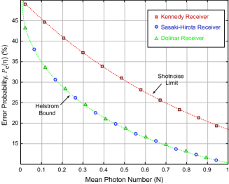
Figure 1: Monte carlo simulation of the Kennedy, Dolinar and Sasaki-Hirota receivers as a function of the signal amplitude for perfect photon counting with $\xi_{0}=\xi_{1}=\frac{1}{2}$. As expected, the Dolinar and Sasaki-Hirota protocols both achieve the Helstrom bound while the Kennedy receiver is approximately a factor of two worse.

Monte Carlo simulations of the Kennedy, Sasaki-Hirota and Dolinar receivers were performed to verify the above quantum efficiency analysis and to analyze the effects of additional detector imperfections. Fig. 1 shows benchmark simulation results for perfect photodetection. The three receivers perform as expected in the small-amplitude regime; both the Sasaki-Hirota and Dolinar protocols achieve the Helstrom bound while the Kennedy receiver is approximately a factor of two worse, at the shotnoise limit . Statistics were accumulated for 10,000 Monte Carlo samples in which $\hat{\rho}_{0}$ and $\hat{\rho}_{1}$ were randomly selected with $\xi_{0}=\xi_{1}=1/2$.

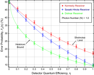
Figure 2: Performance of the Kennedy, Sasaki-Hirota, and Dolinar receivers as a function of the detector quantum efficiency $\eta$. The simulations were performed for $\xi_{0}=\xi_{1}=\frac{1}{2}$ and data points reflect the result of Monte Carlo simulations of the three receivers. Dotted lines correspond to the analytic results derived in Section II and illustrate that the Dolinar receiver achieves the Helstrom bound even for sub-unity quantum efficiency.

Detector imperfections, however, will degrade the performance of each of the three receivers, and here we investigate the relative degree of that degradation for conditions to be expected in practice. The analysis is based on the observation that single photon counting in optical communications is often implemented with an avalanche photodiode (APD), as APDs generally provide the highest detection efficiencies. In the near-infrared, for example, high-gain Silicon diodes provide a quantum efficiency of $\eta\sim 50$%. Additional APD non-idealities include: a dead time following each detected photon during which the receiver is unresponsive, dark counts in the absence of incoming photons due to spontaneous breakdown events in the detector medium, a maximum count rate above which the detector saturates (and can be damaged), and occasional ghost clicks following a real photon arrival— a process referred to as “after pulsing.” For the Dolinar receiver, which requires high-speed signal processing and actuation in order to modulate the adaptive feedback field, delays must also be considered. That is, the optical modulators used to adjust the phase and amplitude of the feedback signal as well as the digital signal processing technology necessary Stockton et al. (2002) for implementing all real-time computations display finite bandwidths.

Fig. 2 compares the error probabilities of the three receivers for sub-unity quantum efficiency but otherwise ideal detection. The mean photon number of the signal, $\Psi_{1}(t)$, in this simulation is $\bar{N}=1$ with $\Psi_{0}(t)=0$ and $\xi_{0}=\xi_{1}=1/2$. Data points in the figure were generated by accumulating statistics for 10,000 Monte Carlo simulations of the three receivers, and the dotted lines correspond to the error probabilities derived in Section II. The simulations agree well with the analytic expressions and it is evident that the Dolinar receiver is capable of achieving the Helstrom bound for $\eta<1$ while the Sasaki-Hirota receiver performance lies between that of the Kennedy and Dolinar receivers.

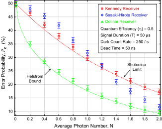
Figure 3: Performance of the Kennedy, Sasaki-Hirota and Dolinar receivers as a function of the mean number of photons in the signal under realistic experimental conditions, including a quantum efficiency of 50%, a dark-count rate of 250 clicks/s, an afterpulsing probability of 1% and feedback delays of 100 ns.

Fig. 3 compares the error probabilities for the three receivers with the additional detector and feedback non-idealities taken into account. Based on the performance data of the Perkin-Elmer SPCM-AQR-13 Si APD single photon counting module, we assumed a maximum count rate of $10^{7}$ photons/s, a detector dead-time of 50 ns, a dark count rate of 250 clicks/s and an after-pulsing probability of 1%. For the Dolinar receiver, it was assumed that there was a 100 ns feedback delay resulting from a combination of digital processing time and amplitude/phase modulator bandwidth. The data points in Fig. 3 correspond to the error probabilities generated from 10,000 Monte Carlo simulations with $\xi_{0}=\xi_{1}=1/2$. The lower dotted line indicates the appropriate Helstrom bound as a function of the mean photon number, $\bar{N}$, for a detector with quantum efficiency, $\eta=0.5$, and the upper curve indicates the analogous Kennedy receiver error. Evidentally, technical imperfections can have a large negative effect on the performance of passive detection protocols like the Kennedy and Sasaki-Hirota receivers while the Dolinar receiver is more robust.

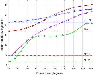
Figure 4: Error probabilities for the Dolinar receiver as a function of the phase error in the signal state corresponding to logical 1 for different mean photon numbers. Monte Carlo data points were generated by accumulating statistics for 10,000 random bits. Solid lines are a fit to the data.

Unlike open-loop procedures, however, the feedback nature of the Dolinar receiver additionally requires precise knowledge of the incoming signal phase, $\varphi$, so that $U^{*}(t)$ can be properly applied. Fluctuations in the index of refraction of the communication medium generally lead to some degree of phase noise in the incoming signal, $\Psi(t)$. Adequately setting the phase of $U(t)$ necessarily requires that some light from the channel be used for phase-locking the local oscillator— a task that reduces the data transmission bandwidth. Therefore, operating a communication system based on the Dolinar receiver at the highest feasible rate requires that the number of photons diverted from the data stream to track phase variations in the channel be minimized. This optimization in turn requires knowledge of how signal phase noise propagates into the receiver error probability.

Figure 4 shows the error probability, $P_{\mathrm{D}}(\delta\varphi)$ as a function of the phase difference, $\delta\varphi$, between the incoming signal and the local oscillator. Data points correspond to results from 10,000 Monte Carlo simulations per photon number and phase angle, and the solid curves reflect numerical fits to the Monte Carlo points. An exact comparison between the open-loop and Dolinar receivers requires information regarding the specific phase-error density function for the actual communication channel being utilized. However, we do note that at $\bar{N}=1$ photon, the phase of the local oscillator could be as large as $\delta\varphi\sim 25^{\circ}$ before its error probability increased to that of the Kennedy receiver. Additionally, it appears that the slope of $P_{\mathrm{D}}(\delta\varphi)$ is zero at $\delta\varphi=0$ which implies that the Dolinar receiver conveniently displays minimal sensitivity to small phase fluctuations in the channel.

IV Discussion and Conclusions

The Dolinar receiver was found to be robust to the types of detector imperfections likely to exist in any real implementation of a binary communication scheme based on optical coherent state signaling and photon counting. This robustness seemingly results from the fact that the Dolinar receiver can correct itself after events that cause an open-loop receiver to irreversibly misdiagnose the transmitted state. For example, imperfect detection efficiency introduces a failure mode where the probability, $p(H_{0}|\hat{\rho}_{1})$, is increased above the value set by quantum mechanical vacuum fluctuations. However, the optimal structure of the Dolinar receiver feedback insures that it still achieves the quantum mechanical minimum because it has control over the counting rate. That is, if the Dolinar receiver selects the wrong hypothesis at some intermediate time, $t_{k}<T$, the structure of the feedback insures that the receiver achieves the highest allowable probability for invalidating that incorrect decision during the remainder of the measurement, $t_{k}<t\leq T$.

In the opposite situation, where dark counts or background light produce detector clicks when there is no signal light in the channel, open-loop receivers will decide in favor of $\hat{\rho}_{1}$ without any possibility for self-correction. This type of error leads to an irreparable open-loop increase in $p(H_{1}|\hat{\rho}_{0})$. But, the Dolinar receiver has the potential to identify and fix such a mistake since selecting the wrong hypothesis at intermediate times increases the probability that a future click will invalidate the incorrect decision. When background light is present, poor phase coherence between stray optical fields and the signal provides no enhanced open-loop discrimination as there is no local oscillator to establish a phase reference; a received photon is a received photon (assuming that any spectral filtering failed to prevent the light from hitting the detector). The Dolinar receiver is better immune to such an error since since incoherent addition of the stray field to the local oscillator will generally reduce the likelihood of a detector click, and even if so, that click will be inconsistent with the anticipated counting statistics.

Despite the previous belief that the Dolinar receiver is experimentally impractical due to its need for real-time feedback, we have shown that it is rather attractive for experimental implementation. Particularly, quantum efficiency scales out of a comparison between the Dolinar receiver error and the Helstrom bound, while this is not the case for known unitary rotation protocols. These results strongly suggest that real-time feedback, previously cited as the Dolinar receiver’s primary drawback, in fact offers substantial robustness to many common imperfections that would be present in a realistic experimental implementation. Most importantly, simulations under these realistic conditions suggest that the Dolinar receiver can out-perform the Kennedy receiver with currently available experimental technology, making it a viable option for small-amplitude, minimum-error optical communication.