Tomographic measurements on superconducting qubit states

Abstract

We propose an approach to reconstruct any superconducting charge qubit state by using quantum state tomography. This procedure requires a series of measurements on a large enough number of identically prepared copies of the quantum system. The experimental feasibility of this procedure is explained and the time scales for different quantum operations are estimated according to experimentally accessible parameters. Based on the state tomography, we also investigate the possibility of the process tomography.

I introduction

The generation of superpositions of macroscopic quantum states in superconducting devices jr ; Nakamura ; pashkin ; chiorescu ; han have motivated further research on quantum information processing in these systems. Two types of superconducting qubits based on Josephson junction devices have been proposed and experimentally demonstrated. One involves two Cooper-pair charge states in a small superconducting island connected to a circuit by a Josephson tunnel junction and a gate capacitor (see, e.g., Nakamura ; pashkin ; makhlin ). An alternative approach is based on the phase states of a Josephson junction or the flux states in a ring superconducting structure ioffe ; chiorescu ; han . Further, experimental observations on quantum oscillations and the demonstration of conditional gate operations in two coupled charge qubits pashkin are necessary first steps towards future realizations of quantum information processors.

A crucial step in quantum information processing is the measurement of the output quantum states. However, a quantum state cannot be ascertained by a single quantum measurement. This is because quantum states may comprise many complementary features which cannot be measured simultaneously and precisely due to uncertainty relations. However, all complementary aspects can in principle be observed by a series of measurements on a large enough number of identically prepared copies of the quantum system. Then we can reconstruct a quantum state from such a complete set of measurements of system observables (i.e., the quorum qu ). Such a procedure is called “reconstruction of quantum states” or Quantum State Tomography (QST).

Quantum state tomography is not only important for quantum computation, which requires the verification of the accuracy of quantum operations, but it is also important for fundamental physics. Many theoretical studies for tomographic reconstruction of quantum states have been done, e.g. references theor ; dfv ; long ; Ariano . Experimentally, tomography has been investigated for a variety of systems, including: e.g., the vibrational state of molecules dunn , the motional quantum state of a trapped atom lei ; kur , two-photon states white , the electromagnetic field smithey , and rare-earth-metal-ion-based solid-state qubit jjl , the two-qubit states in the trapped ions cfr . The quantum states of multiple spin-$\frac{1}{2}$ nuclei have also been measured in the high-temperature regime using NMR techniques chuang ; miquel ; cory .

For continuous variable cases (e.g., the molecular vibrational mode dunn , motional quantum states of a trapped ion lei ; kur , a single-mode smithey of the electromagnetic field), the quantum states can be known by the tomographic measurement of their Wigner function. For the discrete variable case (e.g., in NMR systems), the measurements on the density matrix in NMR experiments are realized by the NMR spectrum of the linear combinations of “product operators”, i.e. products of the usual angular momentum operators cory .

Based on the state tomography, a quantum “black box” connected to an unknown external reservoir can also be characterized. This “black box” transfers any known input state to an unknown output state. The determination of the quantum transfer function for this ‘black box” is called quantum process tomography il . This procedure needs to input a large enough number of different known states into the “black box”, then to make tomographic measurements on output states, finally to obtain the quantum transfer function, which determines the “black box”. This procedure would be very important for the case when the noisy channel is unclear. Process tomography has been experimentally realized, e.g., in optical systems mwm , NMR ysw .

To our knowledge, there is no adequate theoretical analysis or experimental demonstration for the reconstruction of qubit states in solid state systems, besides our recent work in Ref. liu . There, we considered a very general class of spin Hamiltonians used to model generic solid state systems liu . Here, the emphasis is not on a general model but on a specific system: superconducting qubits. Recent technical progress makes it possible to realize quantum control in superconducting quantum devices and ascertain either the charge Nakamura ; pashkin or the flux chiorescu qubit states. Furthermore, practical experiments on quantum computing require the knowledge of the full information of the quantum state, so the reconstruction of quantum states in solid state systems is a very important issue.

In this paper, we analyze how to reconstruct charge qubit states in superconducting circuits. In principle, if all qubits can be measured at same time in superconducting circuits as in optical systems (e.g., Ref. dfv ), then only single-qubit operations are enough to assist the implementation of the reconstruction of any multiple-qubit state. However, our proposal only considers one qubit measurement at a time. This is because simultaneous measurements of many qubits are currently very difficult to implement comments in superconducting circuits. Another reason is that simultaneous measurements require many probes in contact with qubits, inducing more noisy channels. These multiple noisy channels will quickly reduce the coherence of the qubit states, decreasing the accuracy of the reconstructed states. So for two-qubit and multi-qubit state tomography, appropriate two-qubit operations are necessary, due to the constraint of a single-qubit measurement at a time.

Although our analysis of the tomographic reconstruction of charge qubit states might seem somewhat similar to the one used for NMR systems chuang ; miquel ; cory , there are significant differences on how to realize the state tomography in Josephson junction (JJ) charge qubits. For example, NMR QST (like optical QST) also only involves single-qubit operations. A question we will focus on is the following: is it possible to do QST with the currently accessible experimental capability on JJ qubits? In view of the short relaxation and decoherence times, it is also necessary to estimate quantum operation times required for reconstructing charge qubit states. In particular, it is not trivial to find an appropriate two-qubit operation to realize all two and multiple qubit measurements.

Here, we theoretically analyze in detail the necessary experimental steps for the tomographic reconstruction of dc-SQUID-controlled charge qubit states. This analysis can be easily generalized to other proposals of controllable superconducting qubits (e.g., flux and phase qubits). In Sec. II, the reconstruction of single-qubit states is described in detail. The time scales of operations for measurements of all three unknown matrix elements are also estimated by using currently accessible experimental parameters. In Sec. III, all operations required to reconstruct two-qubit states are given, the time scales for the first and second qubit measurements are estimated using experimentally accessible parameters. In Sec. IV, using an example, we generalize our two-qubit tomography to the multiple-qubit case. Finally in Sec. V, we discuss the “process tomography” of singe-qubit charge systems based the “state tomography”. Sections III, IV, and V contain our most important results. The conclusions and further discussions are given in sections VI and VII, respectively.

II reconstruction of single-qubit states

The content of this section on single-qubit operations and the reconstruction of single-qubit states is known book to specialists in the optical, NMR and other areas (e.g, qu ; theor ; dfv ; long ; Ariano ; dunn ; lei ; kur ; white ; smithey ; jjl ; cfr ; chuang ; miquel ; cory ), where the QST is extensively studied. But here we specify a detailed description of the steps needed for the experimental realization of the tomographic reconstruction for charge qubit states. This should be helpful to solid state experimentalists who are not specialists on the QST.

II.1 Theoretical model and single-qubit states

We consider a controllable dc-SQUID system which consists of a small superconducting island with $n$ excess Cooper-pair charges, connected by two nominally-identical ultra-small Josephson junctions; each having capacitance $C^{0}_{J}$ and Josephson coupling energy $E^{0}_{J}$. A control gate voltage $V_{g}$ is coupled to the Cooper-pair island by a gate capacitance $C_{g}$. The qubit is assumed to work in the charge regime, e.g., the single-electron charging energy $E_{C}=e^{2}/2(C_{g}+2C^{0}_{J})$ and Josephson coupling energy $E^{0}_{J}$ satisfy the condition $E_{C}\gg E_{J}$. If the applied gate voltage range $V_{g}$ is near a value $V_{g}=e/C_{g}$, only two charge states, denoted by $n=0$ and $n=1$, play a key role, then this charged box is reduced to a two-level system (qubit) whose dynamical evolution is governed by the Hamiltonian makhlin ; y

$$H=-\,\frac{1}{2}\,\delta\!E_{\rm ch}(n_{\rm g})\,\sigma_{z}-\frac{1}{2}E_{\rm J}(\Phi_{x})\,\sigma_{x},$$ (1)

where we adopt the convention of charge states $|0\rangle=|\!\uparrow\rangle$ and $|1\rangle=|\!\downarrow\rangle$. The charge energy $\delta\!E_{\rm ch}(n_{\rm g})=4\,E_{\rm C}(1-2n_{\rm g})$ with $n_{\rm g}=C_{\rm g}V_{\rm g}/2e$ can be controlled by the gate voltage $V_{\rm g}$. The Josephson coupling energy $E_{\rm J}(\Phi_{x})=2\,E^{0}_{\rm J}\cos(\pi\Phi_{x}/\Phi_{0})$ is adjustable by the external flux $\Phi_{x}$, and $\Phi_{0}=h/2e$ is the flux quantum. Our goal here is to determine any single charge qubit state by the controllable dynamical operation governed by the Hamiltonian (1).

Any single-qubit state (mixed or pure) can be represented by a density matrix operator in a basis $\{|0\rangle=|\!\uparrow\rangle,\,|1\rangle=|\!\downarrow\rangle\}$ as

$$\rho = \left(\begin{array}[]{cc}\rho_{00}&\rho_{01}\\ \rho_{10}&\rho_{11}\end{array}\right)=\frac{1}{2}\sum_{k=0,x,y,z}r_{k}\,\sigma_{k},$$ (2c)

or

$$\rho = \rho_{00}\,|0\rangle\langle 0|+\rho_{01}\,|0\rangle\langle 1|+\rho_{10}\,|1\rangle\langle 0|$$ (2d)

$$+ \rho_{11}\,|1\rangle\langle 1|,$$

where $\sigma_{k=x,y,z}$ are Pauli operators and $\sigma_{k=0}$ is an identity operator. Four real parameters $r_{k}\,\,(k=0,x,y,z)$ can be expressed as

$$r_{0} = \rho_{00}+\rho_{11},\,\,\,\,\,\,\,\,\,\,\,\,\,\,\,\,r_{x}=\rho_{01}+\rho_{10},$$

$$r_{y} = i(\rho_{01}-\rho_{10}),\,\,\,\,\,\,\,\,\,\,\,r_{z}=\rho_{00}-\rho_{11}.$$

The normalization condition $\rho_{00}+\rho_{11}=1$ ensures that the qubit (2) can actually be determined by three real parameters $r_{x}$, $r_{y}$, $r_{z}$ corresponding book to a Bloch vector $\overrightarrow{r}$, which satisfies the condition $|\overrightarrow{r}|\leq 1$ (see Fig.1(a)). The state $\rho$ is pure if and only if $|\overrightarrow{r}|=1$. When the state $\rho$ is pure, the Bloch vector $\overrightarrow{r}$ defines a point on the unit three-dimensional sphere.

These three coefficients $r_{k}\,\,(k=x,\,y,\,z)$ can be obtained from measurements of $\sigma_{x}$, $\sigma_{y}$, $\sigma_{z}$. The correspondence between these three measurements and the coefficients $r_{k}$ is given by

$$r_{k}\,=\,{\rm Tr}(\rho\,\,\sigma_{k}),$$

due to the relation ${\rm Tr}(\sigma_{i}\sigma_{j})=2\delta_{ij}$, where $\delta_{ij}$ is the Kronecker delta.

II.2 Quantum operations and measurements on single-qubit states

In principle, the state of the charge qubit can be read by a single-electron transistor (SET) Nakamura ; pashkin ; y coupled capacitively to a charge qubit. Here we consider the ideal case in which the SET is coupled to the qubit only during the measurement. When the SET is coupled to the qubit, the dissipative current $I$ flowing through the SET is proportional to the probability of a projective operator measurement $|1\rangle\langle 1|$ on the qubit state, which has actually been applied by the experiment Nakamura ; pashkin . The $|1\rangle\langle 1|$ measurement is equivalent to a $\sigma_{z}$ measurement on the state $\rho$,

$$p_{1}\,=\,{\rm Tr}(\rho\,|1\rangle\langle 1|)\,=\,\frac{1}{2}[1-{\rm Tr}(\rho\,\sigma_{z})]\,=\,\rho_{11}$$

due to the relation

$$|1\rangle\langle 1|\,=\,\frac{1}{2}(\sigma_{0}-\sigma_{z}).$$

The parameters $r_{0}$ and $r_{z}$ can be determined by the result of the measurement $|1\rangle\langle 1|$, together with the normalization condition.

We can also relate the two other measurement operators, $\sigma_{x}$ and $\sigma_{y}$, to the operator $|1\rangle\langle 1|$ (essentially $\sigma_{z}$), which is the measurement experimentally realized in the charge qubits. This is because the current $I$ flowing through the SET is sensitive to the charge state $|1\rangle$, so the single qubit operations have to be performed so that the desired parameter $r_{x}$ or $r_{y}$ is transformed to the measured diagonal positions.

Now, we describe the steps to measure $r_{x}$ or $r_{y}$. Let us first choose the external flux $\Phi_{x}=0$ and suddenly drive the qubit to the degeneracy point for a time

$$t_{x}=\frac{\hbar\pi}{2\,E_{\rm J}(0)}=\frac{\hbar\pi}{4\,E^{0}_{\rm J}}$$

such that the qubit state can be rotated $-\pi/2$ along the $x$ direction, here $E_{\rm J}(0)=E_{\rm J}(\Phi_{x}=0)$.

The probability $p_{2}$ of the measurement $|1\rangle\langle 1|$ on the rotated state is

$$p_{2} = {\rm Tr}\left(R_{x}(t_{x})\,\,\rho\,\,R^{\dagger}_{x}(t_{x})\,|1\rangle\langle 1|\right)$$ (3)

$$= {\rm Tr}\left(\,\exp\left\{i\frac{\pi}{4}\sigma_{x}\right\}\,\rho\,\exp\left\{-i\frac{\pi}{4}\sigma_{x}\right\}|1\rangle\langle 1|\,\right)$$

$$= {\rm Tr}\left(\rho\,\exp\left\{-i\frac{\pi}{4}\sigma_{x}\right\}|1\rangle\langle 1|\,\,\exp\left\{i\frac{\pi}{4}\sigma_{x}\right\}\,\right)$$

$$= \frac{1}{2}\,(1+r_{y}),$$

where $R_{x}(t_{x})=\exp\left\{iE_{J}(0)\sigma_{x}t_{x}/2\hbar\right\}$, Eq. (3) means that the measurement $|1\rangle\langle 1|$ on the state rotated $-\pi/2$ along the $x$ direction is equivalent to the measurement $\sigma_{y}$, and the rotation $-\pi/2$ of the qubit is equivalent to an inverse rotation of the measuring instrument, see Fig.  1.

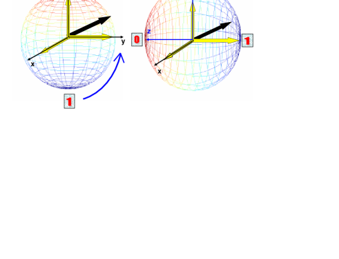
Figure 1: (Color on line) The black Bloch vector indicates a qubit state; the (yellow arrows) $r_{x},\,r_{y}\,$ and $r_{z}$ represent the three components of the Bloch vector along the $x,\,y$ and $z$ axes. The $0$ and $1$ in the north and south poles of the Bloch sphere denote the measured states $|0\rangle$ and $|1\rangle$, respectively. The measurement instrument is attached to a pole (e.g., “1”) of the sphere. A $-\pi/2$ rotation of the qubit state along the $x$ direction is equivalent to a $\pi/2$ rotation of the measuring instrument along the $x$ direction.

In order to make the third measurement $\sigma_{x}$, the qubit state needs now to be rotated $-\pi/2$ (or $\pi/2$) along the $y$ direction. This can be done (e.g., $-\pi/2$ rotation) as follows:

(i)    Set $\Phi_{x}=\Phi_{0}/2$ and $n_{\rm g}=0$; let the system evolve a time $t_{z,1}=\hbar\pi/8E_{\rm C}$ such that a rotation of $-\pi/2$ along the $z$ direction is realized.

(ii)   After the time $t_{z,1}$, set $\Phi_{x}=0$ and $n_{\rm g}=1/2$ and let the system evolve a time period $t_{x,1}=\hbar\pi/2E_{\rm J}(0)=\hbar\pi/4E^{0}_{\rm J}$ such that the system rotates $-\pi/2$ along the $x$ direction.

(iii)   Set $\Phi_{x}=0$ and $n_{\rm g}=1/2$ again and let the system evolve a time $t_{z,2}=3\hbar\pi/8E_{\rm C}$ and a rotation $-3\pi/2$ along the $z$ direction is obtained.

Combining the above three steps, shown in Fig. 2, a $-\pi/2$ rotation of the qubit along the $y$ direction is realized.

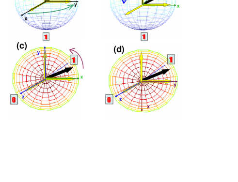
Figure 2: (Color on line) The Bloch vector is the same as Fig. 1. A $-\pi/2$ rotation of the qubit along the $y$ direction is equivalently realized by the rotation $\pi/2$ of the measuring instrument along the $z$ direction (from (a) to (b)), then a $\pi/2$ rotation along the $x$ direction (from (b) to (c)), and a $3\pi/2$ rotation along $z$ direction (from (c) to (d)).

(iv)   After the above rotations, a measurement $|1\rangle\langle 1|$ on this rotated state must be made, which is equivalent to measuring $\sigma_{x}$. Then, the measured probability becomes

$$p_{3} = {\rm Tr}(\,R_{z,x,z}\,\rho\,R^{\dagger}_{z,x,z}\,|1\rangle\langle 1|\,)$$

$$= {\rm Tr}\left(\,\exp\left\{i\frac{\pi}{4}\sigma_{y}\right\}\rho\exp\left\{-i\frac{\pi}{4}\sigma_{y}\right\}|1\rangle\langle 1|\,\right)$$

$$= \frac{1}{2}\,(1+r_{x})$$

with $R_{z,x,z}=R_{z}(t_{z,1})R_{x}(t_{x,1})R_{z}(t_{z,2})$, and

$$R_{z}(t_{z,1}) = \exp\left\{i\frac{2E_{\rm C}}{\hbar}\sigma_{z}t_{z,1}\right\}=\exp\left\{i\frac{\pi}{4}\sigma_{z}\right\},$$

$$R_{x}(t_{x,1}) = \exp\left\{i\frac{E^{0}_{\rm J}}{\hbar}\sigma_{x}t_{x,1}\right\}=\exp\left\{i\frac{\pi}{4}\sigma_{x}\right\},$$

$$R_{z}(t_{z,2}) = \exp\left\{i\frac{2E_{\rm C}}{\hbar}\sigma_{z}t_{z,2}\right\}=\exp\left\{i\frac{3\pi}{4}\sigma_{z}\right\}.$$

We explained how to measure the single qubit states by single qubit operations and measuring $|1\rangle\langle 1|$. Below, we give an example that shows a reconstructed single-qubit state can be graphically represented, and we further give estimates of the operation times to obtain each of the matrix elements of single-qubit states.

II.3 An example

The three measurement results ($p_{1},\,\,p_{2},\,\,p_{3}$) can be used to obtain four coefficients ($r_{0},\,\,r_{x},\,\,r_{y},\,\,r_{z}$) that define a single-qubit state. A single-qubit state can be reconstructed following the steps presented above and an example is described here. If we obtain $r_{x}=1$, $r_{y}=\sqrt{3}$, $r_{z}=1$ by the three experimentally measured probabilities ($p_{1}$, $p_{2}$ and $p_{3}$) on a quantum ensemble of an unknown charge qubit state $\rho$, then

$$\rho_{00} = \rho_{11}\,=\,\frac{1}{2},$$

$$\rho_{01} = \frac{1}{4}\left(1-i\sqrt{3}\right),$$

$$\rho_{10} = \frac{1}{4}\left(1+i\sqrt{3}\right).$$

Thus, the reconstructed state $\rho$ can be written as

$$\rho = \frac{1}{2}\left(|0\rangle\langle 0|+|1\rangle\langle 1|\right)+\frac{1}{4}\left[\left(1+i\sqrt{3}\right)|1\rangle\langle 0|\right]$$

$$+ \frac{1}{4}\left[\left(1-i\sqrt{3}\right)|0\rangle\langle 1|\right]$$

whose real $\rho^{\rm(R)}_{ij}$ and imaginary $\rho^{\rm(I)}_{ij}$ parts are graphically represented in Fig. 3.

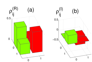
Figure 3: Graphical representation of the density matrix $\rho$ for single-qubit states, see the example explained in section II. The real $\rho_{ij}^{\rm(R)}$ and imaginary $\rho_{ij}^{\rm(I)}$ parts of the density matrix elements $\rho_{ij}=\langle i|\rho|j\rangle$ $(i,\,j=0,1)$ are plotted in (a) and (b), respectively.

II.4 Operation time estimates

The coherent operations required for the tomographic measurements are limited by the decoherence time $T_{2}$. Now let us explore whether the single-qubit state can be reconstructed with the current experiments. To estimate the corresponding time scales for quantum operations to obtain the measurements of $\sigma_{y}$ and $\sigma_{x}$, we first take the suggested parameters from Ref. y , that is, $E^{0}_{\rm J}=100$ mK (about $8.6\,\mu$eV or $2.08$ GHz) and $E_{\rm C}=1$ K (about $86\,\mu$eV or $20.8$ GHz). Here, we use temperature units for energies as in reference y . Thus the approximate time scales of one-qubit operations to obtain $r_{y}$ and $r_{x}$ are

$$t_{x}\approx 5.9\times 10^{-11}\,\,{\rm s}$$

and

$$t_{y}=t_{z,1}+t_{x,1}+t_{z,2}\approx 7.1\times 10^{-11}\,\,{\rm s}.$$

These time scales, required to reconstruct the single-qubit states, are within the measured values Nakamura ; pashkin of the decoherence time $T_{2}$ (of the order of magnitude of ns) of single-qubit charge states.

Now let us consider another set of experimental values. For example, if the Josephson and charge energies are taken (second paper in Ref. pashkin ) as $2E^{0}_{\rm J}=45\mu$eV (about $520$ mK or $10.9$ GHz) and $4E_{\rm C}=580\mu$eV (about $6.73$ K or $140$ GHz), then the time scales required to reconstruct single-qubit states are about $t_{x}\approx 2.3\times 10^{-11}$s and $t_{y}\approx 3.0\times 10^{-11}$s, which are within the decoherence time $T_{2}=5$ ns obtained by that experiment pashkin .

If we take the Josephson and charge energies from in Ref. lehnert , that is, $2E^{0}_{\rm J}/h=13.0$ GHz (about $625$ mK or $53.7$ $\mu$eV) and $4E_{\rm C}/h=149.1$ GHz (about $7.16$ K or $618$ $\mu$eV), then the time scales required to reconstruct single-qubit states are about $t_{x}\approx 1.9\times 10^{-11}$s and $t_{y}\approx 2.6\times 10^{-11}$s, which are also less than one order of magnitude of the decoherence time $T_{2}=325$ ps measured by that experiment lehnert .

III reconstruction of two-qubit states

III.1 Theoretical model and two-qubit states

In this section, we focus on the reconstruction of two-qubit charge states. Any two-qubit state $\rho_{1}$ can be characterized by a density matrix operator

$$\rho_{1}=\frac{1}{4}\sum_{i,j=0,x,y,z}r_{i,j}\,\sigma_{1i}\otimes\sigma_{2j}$$ (4)

where the $16$ parameters $r_{i,j}$ are real numbers. The normalization property of the quantum state requires that $r_{0,0}=1$, so the state $\rho_{1}$ in Eq. (4) can in principle be reconstructed prove by $15$ measurements described by the operators $\sigma_{1i}\otimes\sigma_{2j}$, where all $i$ and $j$ are not simultaneously taken to be $0$. If one of $\sigma_{1i}$ ($i=0,\,x,\,y,\,z$) or $\sigma_{2j}$ ($i=0,\,x,\,y,\,z$) is an identity operator among the measurement operators $\sigma_{1i}\otimes\sigma_{2j}$, we call such a measurement a single-qubit measurement and only write out the non-identity Pauli operator in the following expressions. For example, the operator $\sigma_{1x}\otimes\sigma_{20}$ is called $\sigma_{x}$ measurement of the first qubit, and abbreviated by $\sigma_{1x}$. So there are nine two-qubit measurements among measurements $\sigma_{1i}\otimes\sigma_{2j}$. Recall that only one-qubit is involved during the measurement process in our approach. If we want to obtain these nine two-qubit measurements, then two-qubit operations must be applied dpd such that the singe-qubit measurement can be equivalently transformed into expected two-qubit measurements.

Now our task is to find a non-local two-qubit operation and use this operation to realize all necessary two-qubit measurements on two-qubit states. Here we consider a model proposed by Makhlin et al. makhlin , where two charge qubits are coupled in parallel to a common inductor with inductance $L$. The Hamiltonian makhlin is

$$H = -\,\frac{1}{2}\sum_{l=1}^{2}\left[\delta\!E_{\rm ch}(n_{l,{\rm g}})\,\sigma_{lz}+{E}_{\rm J}(\Phi_{lx})\,\sigma_{lx}\right]$$ (5)

$$- E_{\rm int}(\Phi_{1x},\Phi_{2x})\,\sigma_{1y}\otimes\sigma_{2y},$$

where it is assumed that both qubits are identical, so the charge energies $\delta\!E_{\rm ch}(n_{l,{\rm g}})$ and Josephson coupling energies $E_{\rm J}(\Phi_{lx})$ take the same form as in Eq. (1), but now $\delta\!E_{\rm ch}(n_{l,{\rm g}})$ and $E_{\rm J}(\Phi_{lx})$ for each qubit can be separately controlled by the gate voltages and external fluxes. The interaction energy $E_{\rm int}$ for two coupled qubits can be written as

$$E_{\rm int}(\Phi_{1x},\Phi_{2x})=\frac{E_{\rm J}(\Phi_{1x})E_{\rm J}(\Phi_{2x})}{E_{\rm L}}$$

with

$$E_{\rm L}=\left(\frac{C^{0}_{\rm J}}{C_{\rm qb}}\right)^{2}\left(\frac{\Phi^{2}_{0}}{\pi^{2}L}\right)$$

and $C^{-1}_{\rm qb}=(2C^{0}_{\rm J})^{-1}+C^{-1}_{\rm g}$. Thus, the interaction between the two qubits can be controlled by two external fluxes $\Phi_{lx}$ applied to each qubit.

III.2 Quantum operations and measurements on two-qubit states

Now, we discuss how to reconstruct two-qubit states from the experimental measurements $(|1\rangle\langle 1|)_{l}\,\,(l=1,\,2)$. Single charge qubit operations can be realized by controlling the gate voltage and Josephson couplings. However the two-qubit operations need to couple a pair of interacting charge qubits. The realization of the coupling of two charge qubits have to simultaneously turn on the Josephson couplings of the two charge qubits in Eq. (5), then $\sigma_{lx}$ terms have to be included in the two-qubit operation. However the charge energies for two qubits can be switched off by applying gate voltages such that $n_{l,{\rm g}}=1/2$ ($l=1,\,2$), so a two-qubit operation can be governed by a simpler Hamiltonian

$$H^{\prime}=-\frac{1}{2}\sum_{l=1,2}E_{\rm J}(\Phi_{lx})\,\sigma_{lx}-E_{\rm int}(\Phi_{1x},\Phi_{2x})\,\sigma_{1y}\otimes\sigma_{2y},$$ (6)

where charging energies are set to zero, $\delta E_{\rm ch}(n_{l,{\rm g}})=0$ ($l=1,\,2$), with $n_{1,{\rm g}}=n_{2,{\rm g}}=1/2$, and the external magnetic fields are chosen such that

$$\Phi_{1x}=\Phi_{2x}\neq\frac{\pi}{2}(2q+1)\Phi_{0}$$

with the positive integer number $q$. The coupling $E_{\rm int}(\Phi_{1x},\Phi_{2x})$ can be controlled by the external fluxes $\Phi_{1x}$ and $\Phi_{2x}$.

The basic two-qubit operation can be given by the time-evolution operator $U(t)=\exp\{-iH^{\prime}t/\hbar\}$, which can be written by using the Pauli operators as

$$U(t)\,=\,\frac{1}{2}\left(\cos\phi^{\prime}+\cos\theta^{\prime}\right)I+in_{z}\frac{\sin\theta^{\prime}}{2}\left(\sigma_{1x}+\sigma_{2x}\right)$$

$$+\,i\frac{\sin\phi^{\prime}-n_{x}\sin\theta^{\prime}}{2}\,\sigma_{1z}\otimes\sigma_{2z}$$

$$+\,i\frac{\sin\phi^{\prime}+n_{x}\sin\theta^{\prime}}{2}\,\sigma_{1y}\otimes\sigma_{2y}$$

$$\,-\,\frac{\cos\phi^{\prime}-\cos\theta^{\prime}}{2}\,\sigma_{1x}\otimes\sigma_{2x},$$ (7)

where

$$\phi^{\prime} = \frac{t}{\hbar}\,E_{\rm int}(\Phi_{1x},\Phi_{2x}),\,\,\,\,\,n_{z}=\frac{a}{\sqrt{1+a^{2}}},$$

$$n_{x} = \frac{1}{\sqrt{1+a^{2}}},\,\,\,\,\,\,\,a=\frac{E_{\rm J}}{E_{\rm int}(\Phi_{1x},\Phi_{2x})},$$

$$\theta^{\prime} = \frac{2}{\hbar}\,E_{\rm int}(\Phi_{1x},\Phi_{2x})\,\sqrt{1+a^{2}}\,.$$

Since the two external fluxes satisfy the condition $\Phi_{1x}=\Phi_{2x}$, we let $E_{\rm J}(\Phi_{1x})=E_{\rm J}(\Phi_{2x})=E_{\rm J}$ in the expression Eq. (III.2) for the two-qubit operation. The physical meaning of the angles $\theta^{\prime}$ and $\phi^{\prime}$ becomes clearer by virtue of the “conjugation-by-$\frac{\pi}{4}\Sigma"$ operation lidar on the time evolution operator $U(t)$, which is defined as

$$U^{\prime}(t)=\exp\left\{i\frac{\pi}{4}(\sigma_{1y}+\sigma_{2y})\right\}U(t)\exp\left\{-i\frac{\pi}{4}(\sigma_{1y}+\sigma_{2y})\right\},$$

here, $\Sigma=\sigma_{1y}+\sigma_{2y}$. In the conjugate representation, the time evolution $U^{\prime}(t)$ corresponds to rotations so around the $y$ axis by an angle $\phi^{\prime}$ and the $(n_{x},0,n_{z})$ axis by an angle $\theta^{\prime}$. By choosing the duration $t$ and tuning the values of $E_{\rm J}$ and $E_{\rm int}(\Phi_{1x},\Phi_{2x})$, we can obtain any desired two-qubit operation.

From Eq. (4), it is known that six single-qubit measurements $\{\sigma_{1i},\sigma_{2j}\}$ with $i,j=x,y,z$ and nine two-qubit measurements $\{\sigma_{1i}\otimes\sigma_{2j}\}$ with $i,j=x,\,y,\,z$ are enough to obtain fifteen parameters $r_{i,j}$ of the two-qubit state $\rho_{1}=\frac{1}{4}\sum_{i,j=0,x,y,z}r_{i,j}\,\sigma_{1i}\otimes\sigma_{2j}$. The single-qubit measurements $(|1\rangle\langle 1|)_{l}=\frac{1}{2}(\sigma_{l0}-\sigma_{lz})$ ($l=1,\,2$) on a given state $\rho_{1}$ can be obtained as follows. Two single-qubit measurements $\sigma_{1z}$ and $\sigma_{2z}$ can be implemented by the direct measurements $(|1\rangle\langle 1|)_{1}$ and $(|1\rangle\langle 1|)_{2}$ on the given state $\rho_{1}$. Other four single-qubit measurements (corresponding to $\sigma_{1x},\,\sigma_{2x},\,\sigma_{1y},\,\sigma_{2y}$) need single-qubit operations.

The single-qubit operations corresponding to measurements $\sigma_{lx}$ and $\sigma_{ly}$ on two-qubit states are the same as measuring $\sigma_{x}$ and $\sigma_{y}$ on single-qubit states. However, in the single qubit operations, we need to switch off the interaction of the two qubits. For example, in order to obtain the measurement $\sigma_{1y}$, we need to switch off the interaction between the two-qubit system by setting the applied external flux $\Phi_{2x}=\pi/2$, and setting the first subsystem at the degeneracy point and evolving a time $t=\hbar\pi/4E^{0}_{J}$. Finally, we make a measurement $(|1\rangle\langle 1|)_{1}$ on the rotated state, then the coefficient $r_{y,0}$ can be obtained by this measured result. The other three measurements can also be obtained by taking single-qubit operations similar to $\sigma_{1y}$.

The single-qubit measurements have been obtained by the measurements $(|1\rangle\langle 1|)_{l}(l=1,2)$ on given states by using appropriate single-qubit operations as described above. In order to find out how to obtain the two-qubit measurements via $(|1\rangle\langle 1|)_{l}$, let us consider the measurements $(|1\rangle\langle 1|)_{l}$ on the given state $\rho_{1}$ performed by a sequence $W$ of single-qubit and two-qubit operations. The corresponding measured probability $p$ can be expressed as

$$p={\rm Tr}\left[W\,\rho_{1}\,W^{\dagger}(|1\rangle\langle 1|)_{l}\right]=\frac{1}{2}-\frac{1}{2}{\rm Tr}\left[\rho_{1}\,W^{\dagger}\sigma_{lz}W\right],$$ (8)

where we show that the measurement $(|1\rangle\langle 1|)_{l}$ on the rotated state $W\rho_{1}\,W^{\dagger}$ may be interpreted as an equivalent measurement $W^{\dagger}\sigma_{lz}W$ ($l=1,2$) on the state $\rho_{1}$. So our task now is to find an appropriate two-qubit operation and apply this two-qubit and single-qubit operations to the measured state $\rho_{1}$, such that we can equivalently obtain the desired two-qubit measurement.

Here, the required two-qubit operation $U(\tau)$ can be obtained by choosing the evolution time $\tau$, the Josephson coupling energies $E_{\rm J}$, and $E_{\rm L}$ in Eq. (III.2) such that $\phi^{\prime}=(2m-1)\pi/4$ and $\theta^{\prime}=n\pi$ where $m,\,n$ are positive integers. The above conditions can be satisfied if the ratio

$$\frac{E_{\rm L}}{E_{\rm J}}=\sqrt{\left(\frac{4n}{2m-1}\right)^{2}-1},$$

and the evolution time $\tau$ is chosen as

$$\tau=\frac{\hbar\pi}{4E_{\rm J}}\sqrt{(4n)^{2}-(2m-1)^{2}}.$$

If we choose the integers $m$ and $n$ to minimize the ratio $E_{\rm L}/E_{\rm J}$, then $E_{\rm L}/E_{\rm J}=\sqrt{15}\cong 3.87$ when $\theta^{\prime}=\pi$ and $\phi^{\prime}=\pi/4$; so the two-qubit operation time $\tau$ is chosen as $\tau=\hbar\pi\sqrt{15}/4E_{\rm J}$. Thus Eq. (III.2) is specified by the time evolution operator

$$U(\tau) = \frac{1}{2\sqrt{2}}\left[\left(1-\sqrt{2}\right)I-\left(1+\sqrt{2}\right)\,\sigma_{1x}\otimes\sigma_{2x}\right.$$ (9)

$$+ \left.i\,\sigma_{1y}\otimes\sigma_{2y}+i\,\sigma_{1z}\otimes\sigma_{2z}\right].$$

Combined with other single qubit rotations, $U(\tau)$ can be used to obtain all the desired coefficients $r_{i,j}$ corresponding to the two-qubit measurements $\sigma_{1i}\otimes\sigma_{2j}$, with $i,\,j=x,\,y,\,z$.

Let us further discuss how to obtain a desired coefficient, for example, $r_{y,y}$ corresponding to the two-qubit measurement $\sigma_{1y}\otimes\sigma_{2y}$. We can take the following steps:

(i)    We switch off the interaction between the first and second qubits by applying an external flux $\Phi_{2x}=\pi/2$, which means $E_{\rm J}(\Phi_{2x})=0$. Now we only manipulate the first qubit such that a rotation $\pi/2$ about the $z$ axis, defined as $Z_{1}=\exp[i\pi\sigma_{1z}/4]$, is performed; this single-qubit operation is described in Section II.

(ii)   Following the single-qubit rotation $Z_{1}$ of the first qubit, the gate voltages are applied such that $n_{1,{\rm g}}=n_{2,{\rm g}}=1/2$, which means that the two qubits work at the degeneracy points. Simultaneously, we turn on and adjust the external fluxes so that the external fluxes $\Phi_{lx}$, energies $E_{\rm L}$ and $E_{\rm J}$ in the two-qubit operation described by the Hamiltonian (6) satisfy the conditions $\Phi_{1x}=\Phi_{2x}\neq\pi(2q+1)/2$ with positive integer $q$ and $E_{\rm L}/E_{\rm J}=\sqrt{15}\cong 3.87$. Afterwards, we let the system evolve a time $\tau=\hbar\pi\sqrt{15}/4E_{\rm J}$; which means that a two-qubit rotation $U(\tau)$ has been performed.

The operation sequence $W=U(\tau)Z_{1}$ described above changes state $\rho_{1}$ into

$$\widetilde{\rho}=U(\tau)\,Z_{1}\,\rho_{1}\,Z^{\dagger}_{1}\,U^{\dagger}(\tau).$$

(iii)   Finally, when a single-qubit measurement $(|1\rangle\langle 1|)_{1}$ is performed on the state $\widetilde{\rho}$, a two-qubit measurement equivalent to $\sigma_{1z}\otimes\sigma_{2y}$ is implemented:

$$Z^{\dagger}_{1}\,U^{\dagger}(\tau)\,(|1\rangle\langle 1|)_{1}\,U(\tau)\,Z_{1}=\frac{1}{2}+\frac{1}{2\sqrt{2}}\left(\sigma_{1z}+\sigma_{1y}\otimes\sigma_{2y}\right).$$

The corresponding measurement probability $\widetilde{p}$ can be given as

$$\widetilde{p}={\rm Tr}\left\{U(\tau)\,Z_{1}\,\rho_{1}\,Z^{\dagger}_{1}\,U^{\dagger}(\tau)(|1\rangle\langle 1|)_{1}\right\}$$

$$=\frac{1}{2}+\frac{1}{2\sqrt{2}}{\rm Tr}\,[\,\rho_{1}\,(\sigma_{1z}+\sigma_{1y}\otimes\sigma_{2y})\,]$$

$$=\frac{1}{2}+\frac{1}{2\sqrt{2}}(r_{z,0}+r_{y,y}).$$ (10)

Because the coefficient $r_{z,0}={\rm Tr}(\rho_{1}\,\sigma_{1z})$, corresponding to the operator $\sigma_{1z}\otimes\sigma_{20}$, has been given by the single-qubit measurement $\sigma_{1z}$, then the coefficient $r_{y,y}={\rm Tr}(\rho_{1}\,\sigma_{1y}\otimes\sigma_{2y})$ is obtained via $\widetilde{p}$ and $r_{z,0}$.

In table 1, we have summarized nine equivalent two-qubit measurements described by $-\sqrt{2}\,W^{\dagger}\sigma_{1z}W$ on the original state $\rho_{1}$, which are obtained by the first qubit measurement $(|1\rangle\langle 1|)_{1}$ on the rotated state $W\rho_{1}W^{\dagger}$ for a sequence $W$ of operations with appropriately-chosen single-qubit and two-qubit operations. We can use the results corresponding to these nine equivalent two-qubit measurements together with the other six single-qubit measurements to obtain all the coefficients corresponding to the two-qubit states, and then obtain any two qubit state.

We can also obtain coefficients $r_{ij}$ ($i,\,j\,\neq 0$) corresponding to all two-qubit measurements by using the second qubit measurement $(|1\rangle\langle 1|)_{2}$. For example, if we make a measurement $(|1\rangle\langle 1|)_{2}$ on the rotated state $\widetilde{\rho}$ considered above, we obtain another equivalent two-qubit measurement, which is expressed as

$$Z^{\dagger}_{1}\,U^{\dagger}(\tau)\,(|1\rangle\langle 1|)_{2}\,U(\tau)\,Z_{1}=\frac{1}{2}+\frac{1}{2\sqrt{2}}(\sigma_{2z}-\sigma_{1x}\otimes\sigma_{2x}).$$

Using this measurement, combined with the single-qubit measurement $\sigma_{2z}$, we can obtain the coefficient $r_{x,x}$ corresponding to the two-qubit measurement $\sigma_{1x}\otimes\sigma_{2x}$. Nine equivalent two-qubit measurements realized by the second qubit $(|1\rangle\langle 1|)_{2}$ have also been summarized in Table 2. Comparing tables 1 and 2 shows that different operations and steps are required in order to obtain the same coefficient for different measurements. For example, in order to obtain $r_{x,z}$, two operation steps are needed for the first qubit measurement $(|1\rangle\langle 1|)_{1}$, but it needs four steps for the second qubit measurement $(|1\rangle\langle 1|)_{2}$.

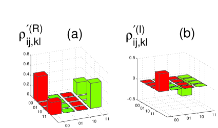
Figure 4: Graphical representation of the density matrix $\rho^{\prime}$ for the two-qubit state described in the example given in section III. The real $\rho^{\prime\rm(R)}_{ij,kl}$ and imaginary $\rho^{\prime\rm(I)}_{ij,kl}$ parts of the density matrix elements for the two-qubit state $\rho^{\prime}$ in the basis $|00\rangle,\,|01\rangle,\,|10\rangle,\,|11\rangle$ are plotted in (a) and (b) respectively.

III.3 An example

We can also give another schematic example for a reconstructed two-qubit state. For instance, according to the operations steps discussed above for the reconstruction of any two-qubit state, if we obtain $r_{x,x}=1/8$, $r_{x,y}=r_{y,x}=\sqrt{3}/8$, $r_{z,z}=1/4$ and $r_{y,y}=-1/8$ from the sixteen measured probabilities on an ensemble of identically prepared copies of a two-qubit system with unknown state $\rho^{\prime}$, then we can reconstruct this unknown state as

$$\rho^{\prime} = \frac{1}{2}[|00\rangle\langle 00|+|11\rangle\langle 11|]+\frac{1}{2}\left(1-i\sqrt{3}\right)|00\rangle\langle 11|$$

$$+ \frac{1}{2}\left(1+i\sqrt{3}\right)|11\rangle\langle 00|,$$

which is graphically shown in Fig.​ (4) with the real $\rho^{\prime\rm(R)}_{ij,kl}$ and imaginary $\rho^{\prime\rm(I)}_{ij,kl}$ parts of the reconstructed state $\rho^{\prime}$, where $i,\,j,\,k,\,l$ can take the values $0$ or $1$.

III.4 Operation time estimates

We can also estimate the operation time required to reconstruct two-qubit states for the Josephson and charge energies y $E^{0}_{\rm J}=100$ mK and $E_{\rm C}=1$ K. We assume that the ratio $E_{\rm L}/E_{\rm J}=\sqrt{15}\cong 3.87$ is obtained by adjusting the external flux $\Phi_{lx}$ ($l=1,\,2$) such that $\Phi_{lx}=0$, which means the ratio between $E_{\rm L}$ and $E^{0}_{J}$ should satisfy the condition $E_{\rm L}/E^{0}_{\rm J}=2\sqrt{15}\cong 7.74$ when the circuits are fabricated. In such case, the realization of the two-qubit operation in Eq. (9) requires a time $\tau\approx 2.32\times 10^{-10}$ s. Our previous estimates for the times to perform $\pi/2$ rotations about the $x$ and $z$ axes are $5.9\times 10^{-11}$ s and $3.0\times 10^{-12}$ s, respectively. Then, using tables 1 and 2, we can estimate the total operation time required for obtaining the coefficients of the two-qubit measurements corresponding to the first or second qubit measurements, respectively. We find that the required operation times for the two-qubit measurements are less than $0.4$ ns for the two-qubit measurements. The decoherence time $T_{2}$ (e.g., the decoherence time of charge qubit is about $5$ ns in reference Nakamura ) experimentally obtained shows that it is possible to reconstruct two-qubit states within the current measurement technology.

At present, completely controllable multi-qubit superconducting circuits are not experimentally achievable. Here, let us consider the operation time estimates based on another controllable model you . In this model, $N$ charge qubits are coupled to a common superconducting inductance $L$. The Hamiltonian of any pair of qubits, say $i$ and $j$, is

$$H^{\prime}=\sum_{k=i,j}(\varepsilon_{k}\sigma^{(k)}_{z}+\epsilon_{k}\sigma^{(k)}_{x})+\chi\sigma^{(i)}_{x}\otimes\sigma^{(j)}_{x},$$ (11)

where the coupling constant $\chi$ can be tuned to zero by changing the flux either through the common inductance $L$, or through the qubit $i$ (or $j$). Moreover, the parameters $\varepsilon_{k}$ and $\epsilon_{k}$ are respectively controlled by the voltage applied to the $k$th qubit and the magnetic flux through the $k$th qubit. The conditional logic gates, e.g., controlled-NOT and controlled-phase-shift gates, can be performed by virtue of only one two-bit operation and also single-qubit operations in this circuit. This approach is more accessible to experiments, facilitating tomographic measurements. According to calculations liu of tomographic measurements for a class of representative quantum computing models of solid state systems, the two-qubit operation required for the realization of the multi-qubit measurements in this circuit can be easily obtained. That is, if the ratio between the Josephson energy $E^{0}_{\rm J}$ and the two-qubit coupling energy $\chi$ is $E^{0}_{\rm J}=2\chi$, when the circuit is fabricated, then a two-qubit operation $\widetilde{U}(\tau^{\prime})=-i\sigma_{1x}\otimes\sigma_{2x}$ can be obtained with the evolution time $\tau^{\prime}\approx 1.2\times 10^{-10}$ s when the Josephson energy is taken as $E^{0}_{\rm J}=100$ mK. Here, we assume that the two charge qubits are identical and the Josephson energies are maximum when the two-qubit operation is performed If the charging energy is taken as $E_{\rm C}=1$ K, then $\pi/2$ rotations around the $z$ and $x$ axes need times $3.0\times 10^{-12}$ s and $5.9\times 10^{-11}$ s, respectively. The operations to get each of the sixteen (single- and two-qubit) measurements can also be obtained for this model by using an approach similar to the one described above, the estimated operation times to obtain all coefficients of the two-qubit measurements are less than $0.3$ ns, which is also within the experimentally obtained decoherence time $T_{2}=5$ ns.

Table 1: Equivalent two-qubit measurements $-\sqrt{2}\,W^{\dagger}\,\sigma_{1z}\,W$ obtained by measuring $(|1\rangle\langle 1|)_{1}$ on the state $W\rho_{1}\,W^{\dagger}$ with a sequence of appropriately-chosen quantum operations $W$.

Two-qubit	Quantum	Equivalent two-qubit
measurement	operation   $W$	measurement
$\sigma_{1x}\otimes\sigma_{2y}$	$U(\tau)$	$\sigma_{1z}+\sigma_{1x}\otimes\sigma_{2y}$
$\sigma_{1x}\otimes\sigma_{2z}$	$X_{1}U(\tau)$	$-\sigma_{1y}+\sigma_{1x}\otimes\sigma_{2z}$
$\sigma_{1x}\otimes\sigma_{2x}$	$U(\tau)Z_{2}$	$\sigma_{1z}-\sigma_{1x}\otimes\sigma_{2x}$
$\sigma_{1y}\otimes\sigma_{2y}$	$U(\tau)Z_{1}$	$\sigma_{1z}+\sigma_{1y}\otimes\sigma_{2y}$
$\sigma_{1y}\otimes\sigma_{2z}$	$X_{1}U(\tau)Z_{1}$	$\sigma_{1x}+\sigma_{1y}\otimes\sigma_{2z}$
$\sigma_{1y}\otimes\sigma_{2x}$	$U(\tau)Z_{1}Z_{2}$	$\sigma_{1z}-\sigma_{1y}\otimes\sigma_{2x}$
$\sigma_{1z}\otimes\sigma_{2y}$	$U(\tau)Z_{1}X_{1}$	$-\sigma_{1y}+\sigma_{1z}\otimes\sigma_{2y}$
$\sigma_{1z}\otimes\sigma_{2z}$	$X_{1}U(\tau)Z_{1}X_{1}$	$\sigma_{1x}+\sigma_{1z}\otimes\sigma_{2z}$
$\sigma_{1z}\otimes\sigma_{2x}$	$U(\tau)Z_{1}Z_{2}X_{1}$	$-\sigma_{1y}-\sigma_{1z}\otimes\sigma_{2x}$

Table 2: Equivalent two-qubit measurements $-\sqrt{2}\,W^{\dagger}\,\sigma_{2z}W$ obtained by measuring $(|1\rangle\langle 1|)_{2}$ on the state $W\,\rho_{1}\,W^{\dagger}$ with a sequence of appropriately-chosen quantum operations $W$.

Two-qubit	Quantum	Equivalent quantum
measurement	operation $W$	measurement
$\sigma_{1x}\otimes\sigma_{2x}$	$U(\tau)Z_{1}$	$\sigma_{2z}-\sigma_{1x}\otimes\sigma_{2x}$
$\sigma_{1y}\otimes\sigma_{2x}$	$U(\tau)$	$\sigma_{2z}+\sigma_{1y}\otimes\sigma_{2x}$
$\sigma_{1z}\otimes\sigma_{2x}$	$U(\tau)X_{1}$	$-\sigma_{2y}+\sigma_{1z}\otimes\sigma_{2x}$
$\sigma_{1x}\otimes\sigma_{2y}$	$U(\tau)Z_{1}Z_{2}$	$\sigma_{2z}-\sigma_{1x}\otimes\sigma_{2y}$
$\sigma_{1y}\otimes\sigma_{2y}$	$U(\tau)Z_{2}$	$\sigma_{2z}+\sigma_{1y}\otimes\sigma_{2y}$
$\sigma_{1z}\otimes\sigma_{2y}$	$U(\tau)X_{1}Z_{2}$	$\sigma_{2x}+\sigma_{1z}\otimes\sigma_{2y}$
$\sigma_{1x}\otimes\sigma_{2z}$	$U(\tau)Z_{1}Z_{2}X_{2}$	$-\sigma_{2y}-\sigma_{1x}\otimes\sigma_{2z}$
$\sigma_{1y}\otimes\sigma_{2z}$	$U(\tau)Z_{2}X_{2}$	$-\sigma_{2y}+\sigma_{1y}\otimes\sigma_{2z}$
$\sigma_{1z}\otimes\sigma_{2z}$	$U(\tau)X_{1}Z_{2}X_{2}$	$\sigma_{2x}+\sigma_{1z}\otimes\sigma_{2z}$

IV Reconstruction of multiple qubit states

In the above two sections, we focused on the reconstruction of the single and two qubits states. In this section, we discuss the reconstruction of any $n$-qubit state. In the multiple qubit charge circuit, the dynamical evolution is governed by the Hamiltonian makhlin

$$H = -\,\frac{1}{2}\,\sum_{l=1}^{n}[\delta\!E_{\rm ch}(n_{l,{\rm g}})\,\sigma_{lz}+{E}_{\rm J}(\Phi_{lx})\,\sigma_{lx}]$$ (12)

$$- \sum_{l<k}E_{\rm int}(\Phi_{lx},\Phi_{kx})\,\sigma_{ly}\otimes\sigma_{ky},$$

where $\delta\!E_{\rm ch}(n_{l,{\rm g}})=4E_{\rm C}(1-2n_{l,{\rm g}})$, $E_{\rm J}(\Phi_{lx})=2E^{0}_{\rm J}\cos(\pi\Phi_{lx}/\Phi_{0})$, and $E_{\rm int}(\Phi_{lx},\Phi_{kx})$ take the same form as in Eq. (5). We also assume $E_{\rm L}/2E^{0}_{\rm J}=\sqrt{15}\cong 3.87$ and the single-qubits are nominally identical. By virtue of the controllable Hamiltonian (12), in principle we can use $(n-1)$ two-qubit operations together with some single-qubit operations to reconstruct any $n$-qubit state, which can also be described by the density matrix operator

$$\rho_{2}=\frac{1}{2^{n}}\sum_{l_{1},l_{2},\cdots,l_{n}=0,x,y,z}r_{l_{1},l_{2},\cdots,l_{n}}\,\sigma_{l_{1}}\otimes\sigma_{l_{2}}\cdots\otimes\sigma_{l_{n}}$$

with $2^{n}$ real parameters $r_{l_{1},l_{2},\cdots,l_{n}}$ corresponding to the measurements $\sigma_{l_{1}}\otimes\sigma_{l_{2}}\cdots\otimes\sigma_{l_{n}}$. But, here, we only show how to obtain a coefficient corresponding to a three-qubit measurement. The generalization to obtain coefficients of multiple qubit measurements is straightforward.

In order to determine a three-qubit state, we need to make, single-qubit, two-qubit, and three-qubit measurements. It is known that all coefficients corresponding to single-qubit and two-qubit measurements can be obtained by using the same operations and measurements $(|1\rangle\langle 1|)_{l=1,\,2\,3}$ as in section I and II. When we make two-qubit operations on, for example, the first and second qubits, the interaction of the third qubit with these two qubits is switched off by the applied flux $\Phi_{3x}=\pi/2$. Now let us show how to obtain the coefficients corresponding to the three-qubit measurements. For example, for the coefficient $r_{x,z,y}$ of the measurement $\sigma_{1x}\otimes\sigma_{2z}\otimes\sigma_{3y}$, we should make the following sequence of quantum operations:

(i)   Switch off the interaction of the third qubit with the first and second qubits by applying the flux $\Phi_{3x}=\pi/2$. Then make a two-qubit operation $U_{12}(\tau)$, with the same form as Eq. (9). We use the subscript “12” to denote two-qubit operations on the first and second qubits.

(ii)    Switch off the interaction between the first and second qubits by setting $\Phi_{2x}=\pi/2$, and making a $\pi/2$ rotation about the $z$ axis for the first qubit.

(iii)   Make another two-qubit rotation $U_{13}(\tau)$ on the first and third qubits by adjusting the external fluxes such that $\Phi_{1x}=\Phi_{3x}=0$. The two-qubit operation $U_{13}(\tau)$ takes the same form as Eq. (9), but the subscript “$2$” of the Pauli operators in Eq. (9) is replaced by the subscript “$3$”. This process can be described as

$$\rho_{2} \,\xrightarrow{U_{12}(\tau)}\,U_{12}(\tau)\,\rho_{2}\,U^{\dagger}_{12}(\tau)\,\xrightarrow{Z_{1}}\,Z_{1}\,U_{12}(\tau)\,\rho_{2}\,U^{\dagger}_{12}(\tau)\,Z^{\dagger}_{1}$$ (13)

$$\,\xrightarrow{U_{13}}\,U_{13}\,Z_{1}\,U_{12}(\tau)\,\rho_{2}\,U^{\dagger}_{12}(\tau)\,Z^{\dagger}_{1}\,U^{\dagger}_{13}\,.$$

(iv)   Finally, make a measurement $(|1\rangle\langle 1|)_{1}$ on the above rotated state, and obtain the equivalent measurement

$$U^{\dagger}_{12}(\tau)\,Z^{\dagger}_{1}\,U^{\dagger}_{13}\,(|1\rangle\langle 1|)_{1}\,U_{13}\,Z_{1}\,U_{12}\,=\frac{1}{2}-\frac{1}{4}\sigma_{1z}+$$

$$+\frac{1}{4}(\sigma_{1x}\otimes\sigma_{2y}+\sigma_{1y}\otimes\sigma_{3y}-\sigma_{1x}\otimes\sigma_{2z}\otimes\sigma_{3y}),$$ (14)

and corresponding measurement result $p^{\prime\prime}$ is

$$p^{\prime\prime}\,=\,\frac{1}{2}-\frac{r_{z,0,0}+r_{x,y,0}+r_{y,0,y}-r_{x,z,y}}{4}\,.$$ (15)

Finally, we can obtain the coefficient $r_{x,y,z}$ based on $p^{\prime\prime}$ and the single and two qubit measurement results $r_{z,0,0}$, $r_{x,y,0}$ and $r_{y,0,y}$, which can be obtained by using the same way described in sections II and III. Other coefficients corresponding to three-qubit measurements can also be obtained by using a similar procedure. According to the estimated time for reconstructing the two-qubit states, we believe that it is also possible to reconstruct the three-qubit states using current technology. Any multiple-qubit can also be reconstructed by sequentially designing the single-qubit and two-qubit operations. The generalization to multiple-qubit is an extension of the procedure that we outlined above.

V quantum process tomography

It is worth briefly reviewing that, based on qubit state tomography, the noisy channel (usually denoted as the “black box”) of the controllable charge qubits can also be determined. This experimental determination of the dynamics of the “black box” is called quantum process tomography il , which can be described as follows:

(i)    Many known quantum states of the system under investigation are input into the “black box”, which is an unknown quantum channel, for example, an arbitrary environment.

(ii)   After a certain time, the output states evolve into unknown states.

(iii)   By using the state tomography, we can ascertain these unknown states.

(vi)   Finally, an unknown quantum channel is determined by the data obtained for the tomographic measurements on these states.

Experimentally, in order to determine the noisy channel of the studied $N$-qubits il , $N^{2}$ known states need to be prepared, and these states must have density matrices which span the space of any allowed input state density matrices.

We have shown that single-qubit state tomography is experimentally accessible. In order to perform quantum process tomography for a single charge qubit. Four kinds of different charge states $|0\rangle$, $|1\rangle$, $(|0\rangle+|1\rangle)/\sqrt{2}$, and $(|0\rangle+i|1\rangle)/\sqrt{2}$ need to be experimentally prepared. These states can be generated in a SQUID-based charge qubit with current experiments Nakamura ; pashkin ; lehnert . Thus, the process tomography of a single charge qubit is achievable using current technology. With further developments of this technique, the process tomography of multiple charge qubits could also be realized, when data from multi-qubit state tomography is obtainable.

VI conclusions

In conclusion, we discuss how to reconstruct charge qubit states via one-qubit measurements using controllable superconducting quantum devices. Detailed operations for reconstructing single- and two-qubit states are presented. Any $n$-qubit state can also be reconstructed by using $n-1$ two-qubit operations similar to Eq. (9) for different qubit pairs and combining these with required single-qubit operations. Thus the non-local two-qubit operation Eq. (9) plays a key role in the reconstruction of the multiple-qubit states. However, this two-qubit operation is not unique for achieving our purpose. We should note that operations to obtain a fixed coefficient corresponding to multiple-qubit measurements are not unique. The measurements $(|1\rangle\langle 1|)_{l}$ ($l=1,\,2,\,\ldots,\,n$) on the given state with fixed operations $W$ are different for each qubit $l$, because $W$ is not symmetric when exchanging $l$. Our proposal can also be generalized to other superconducting charge qubit circuits with the coupling mediated by photons or a tunable oscillator, e.g., Refs. you2 ; wei , or other types of superconducting qubits, e.g., Refs. majer ; izmalkov ; xu ; berkley ; mcdermott .

We find that the longest operation times to obtain the coefficient of single-qubit and two-qubit states are of the order of $0.01$ ns and $0.4$ ns, respectively, which is less than the decoherence time Nakamura $T_{2}=5$ ns. Moreover, the $\pi$ and $\pi/2$ pulses for single-qubit operations can be performed very well, e.g., in the experiments of the charge echo  echo , and NMR-like experiments esteve . Another experimental estimate shows us that the manipulation accuracy can reach $80-90\%$ (e.g., as in the second reference of Ref. Nakamura ). Thus the single-qubit states could be reconstructed and the process tomography should also be accessible in single-qubit charge systems with current experimental capabilities. In principle, the two-qubit states can also be reconstructed by virtue of well-controlled time for the two-qubit operation. We should also note that larger values of the charge energy $E_{\rm ch}$, the Josephson energy $E^{0}_{\rm J}$, and coupling energy $E_{\rm int}(\Phi_{lx},\Phi_{kx})$ can make the operation times shorter. Thus these larger values should be realized in order to facilitate the tomographic reconstruction.

Quantum oscillations and conditional gate operations have been demonstrated in two coupled charge qubits with the interactions pashkin always turned on. Completely controllable two-qubit charge systems have not been realized yet. However, the coupled two charge qubits, allowing on and off switching of the interaction, might be realizable in the future averin . Then our proposal will become realizable. Because the unswitchable two-qubit interaction makes single-qubit operations impossible, our proposed scheme cannot be readily used to the experimental reconstruction of multiple-qubit charge states when the two-qubit interactions are always turned on. However, for the two-qubit circuit with “always-on” interaction, most of the single-qubit parameters majer ; izmalkov ; xu ; berkley ; mcdermott can be tuned. We can adjust these parameters to obtain $15$ different two-qubit operations, and then derive $15$ different measurement equations with these operations on input states. Afterwards, the two-qubit states can finally be determined. The details on how to reconstruct the superconducting two-qubit states with the “always-on” couplings will be presented elsewhere. However, how to reconstruct qubit states in multiple-qubit (more than two qubits) circuits with “always-on” interactions is an open problem.

VII discussions

In our paper, to simplify the algebra, we focus on one particular family of measurements which are constructed by the direct product of the Pauli operators. However, one can conceive that other complete sets of measurements can also be used to do tomography. These different complete sets of measurements can be transformed to each other by unitary operators. In practice, within the duration of the controllable manipulation, the smaller Bloch rotation might be advantageous to speed up the measurements, but it might also decrease the accuracies of the measurements due to a longer measuring time. How to choose suitable sets of operations during the measurement process is an important technical question for the measurement.

It should also be pointed out that here we discuss an ideal case. In practice, the environmental effect is unavoidable, which result in the relaxation (characterized by $T_{1}$) and decoherence (characterized by $T_{2}$) of the qubits. For example, in the single-qubit state tomography, non-negligible $T_{1}$ decreases all three probabilities of the measurements, however non-negligible $T_{2}$ reduces the probabilities of the measurements with rotations about $x$ and $y$ directions book . So the environmental effect on the reconstructed states is required to be considered in practice for more specific model. Further, the required quantum operations, especially two-qubit nonlocal operation, are difficult to accurately implement during the process of experiments. For example, the probabilities of theoretical calculations with qubit operations for the first and second qubit measurements $(|1\rangle\langle 1|)_{1}$ and $(|1\rangle\langle 1|)_{2}$ are related to parameters $r_{i,j}$ of the equivalent measurements shown in tables 1 and  2, however, the measuring results of inaccurately experimental two-qubit operations will actually relate to not only these results shown in tables 1 and  2, but also other extra terms. If these extra terms are not negligible, the reconstructed states might violate the properties of the positive semi-definiteness of the physical state $\rho$. A third error source is the imperfect readout of the charge qubit (for experiments, e.g., using single charge qubit echo , the fidelity of the readout can reach $99\%$). The limited statistical data also affect the reconstruction of the states. All these imperfection can make the reconstructed states violate the important basic properties of the physical states: normalization, Hermiticity, and positivity. In order to reconstruct a physical qubit state, in principle the maximum likelihood estimation of density matrices can be employed to minimize experimental errors. This method can be applied to numerically optimize the experimental data, which has been used in the optical systems mj and more detailed discussions on this method can be referred to a very good Ref. book2 .

When the tomography is processed, the external flux applied to the SQUID needs to be very quickly changed. For instance, the duration for changing $\Phi_{0}/2$ within a SQUID loop should at least be less than the decoherence time. Thus a pulse field magnetometer with a rapid sweep rate may be required in this experiment. If the sweep rate A of the pulse field magnetometer reaches, e.g. $10^{8}$ Oe/s, then the time to change $\Phi_{0}/2$ in the loop needs about $0.25$ ns for a SQUID area of $400(\mu{\rm m})^{2}$.

We also notice that the number of rotations for the measured density matrix elements to a preferable direction (e.g. $y$ instead of $z$) grows exponentially with the number of qubits. How to solve this problem is still an open question.

VIII acknowledgments

We thank X. Hu, J.Q. You, Y.A. Pashkin, O. Astafiev, and J.S. Tsai for their helpful comments and discussions. This work was supported in part by the National Security Agency (NSA) and Advanced Research and Development Activity (ARDA) under Air Force Office of Research (AFOSR) contract number F49620-02-1-0334, and by the National Science Foundation grant No. EIA-0130383.

References

- (1) J.R. Friedman, V. Patel, W. Chen, S.K. Tolpygo and J.E. Lukens, Nature 406, 43 (2000); C.H. van der Wal, A.C.J. ter Haar, F.K. Wilhelm, R.N. Schouten, C.J.M. Harmans, T.P. Orlando, S. Lloyd, and J.E. Mooij, Science 290, 773 (2000); D. Vion, A. Aassime, A. Cottet, P. Joyez, H. Pothier, C. Urbina, D. Esteve, and M.H. Devoret, ibid. 296, 886 (2002).
- (2) Y. Nakamura, Y.A. Pashkin, and J.S. Tsai, Nature 398, 786 (1999); O. Astafiev, Y.A. Pashkin, T. Yamamoto, Y. Nakamura, and J. S. Tsai, Phys. Rev. B 69, 180507(R) (2004).
- (3) Y.A. Pashkin, T. Yamamoto, O. Astafiev, Y. Nakamura, D.V. Averin, and J.S. Tsai, Nature 421, 823 (2003); T. Yamamoto, Y.A. Pashkin, O. Astafiev, Y. Nakamura, and J.S. Tsai, ibid. 425, 941 (2003).
- (4) J.E. Mooij, T.P. Orlando, L. Levitov, L. Tian, C.H. van der Wal, S. Lloyd, Science 285, 1036 (1999); I. Chiorescu, Y. Nakamura, C.J.P.M. Harmans, and J.E. Mooij, ibid. 299, 1869 (2003).
- (5) S. Han, Y. Yu, X. Chu, S. Chu, and Z. Wang, Science 293, 1457 (2001); Y. Yu, S. Han, X. Chu, S. Chu, and Z. Wang, ibid. 296, 889 (2002).
- (6) Y. Makhlin, G. Schön, and A. Shnirman, Nature 398, 305 (1999).
- (7) L. B. Ioffe, V.B. Geshkenbein, M.V. Feigel’man, A.L. Fauchère, and G. Blatter, Nature 398, 679 (1999)
- (8) W. Band and J.L. Park, Am. J. Phys. 47, 188 (1979); Found. Phys. 1, 133 (1970); 339 (1971); G.M. D’Ariano, Phys. Lett. A 268, 151 (2000); G.M. D’Ariano, L. Maccone and M.G.A. Paris, ibid. 276, 25 (2000); V. Buzek, G. Drobny, G. Adam, R. Derka, and P.L. Knight, J. of Mod. Opt. 44, 2607 (1997).
- (9) U. Leonhardt, Phys. Rev. Lett. 74, 4101 (1995); S. Weigert, ibid. 84, 802 (2000); M. Beck, ibid. 84, 5748 (2000); G. Klose, G. Smith, and P.S. Jessen, ibid. 86, 4721 (2001); O. Steuernagel and J.A. Vaccaro, ibid. 75, 3201 (1995); G. M. D’Ariano and P. Lo Presti, ibid. 86, 4195 (2001); U. Leonhardt, Phys. Rev. A 53, 2998 (1996).
- (10) D.F.V. James, P.G. Kwiat, W.J. Munro, and A.G. White, Phys. Rev. A 64, 052312 (2001).
- (11) G.L. Long, H.Y. Yan, and Y. Sun, J. Opt. B 3 376 (2001); L. Xiao and G.L. Long, Phys. Rev. A 66, 052320 (2002); R. Das, T.S. Mahesh, and A. Kumar, ibid. 67, 062304 (2003); Chem. Phys. Lett. 369, 8 (2003); J.S. Lee, Phys. Lett. A 305, 349 (2002).
- (12) G. M. D’Ariano, M.G.A. Paris, and M. F. Sacchi, Adv. in Imaging and Electron Phys. 128, 205 (2003).
- (13) T.J. Dunn, I.A. Walmsley, and S. Mukamel, Phys. Rev. Lett. 74, 884 (1995).
- (14) D. Leibfried, D.M. Meekhof, B.E. King, C. Monroe, W.M. Itano, and D.J. Wineland, Phys. Rev. Lett. 77, 4281 (1996)
- (15) C. Kurtsiefer, T. Pfau, and J. Mlynek, Nature 386, 150 (1997).
- (16) A.G. White, D.F.V. James, P.H. Eberhard, and P.G. Kwiat, Phys. Rev. Lett. 83, 3103 (1999); T. Yamamoto, M. Koashi, S.K. Özdemir, and N. Imoto, Nature 421, 343 (2003).
- (17) D.T. Smithey, M. Beck, M.G. Raymer, and A. Faridani, Phys. Rev. Lett. 70, 1244 (1993); A.I. Lvovsky, H. Hansen, T. Aichele, O. Benson, J. Mlynek, and S. Schiller, ibid. 87, 050402 (2001); S.A. Babichev, J. Appel, and A.I. Lvovsky, ibid. 92, 193601 (2004).
- (18) J.J. Longdell and M.J. Sellars, Phys. Rev. A 69, 032307 (2004).
- (19) C.F. Roos, G.P.T. Lancaster, M. Riebe, H. Häffner, W. Hänsel, S. Gulde, C. Becher, J. Eschner, F. Schmidt-Kaler, and R. Blatt, Phys. Rev. Lett. 92, 220402 (2004).
- (20) I.L. Chuang, N. Gershenfeld, M.G. Kubinec, D.W. Leung, Proc. R. Soc. Lond. A 454, 447 (1998); I.L. Chuang, N. Gershenfeld, and M. Kubinec, Phys. Rev. Lett. 80, 3408 (1998).
- (21) C. Miquel, J.P. Paz, M. Saraceno, E. Knill, R. Laflamme, and C. Negrevergne, Nature 418, 59 (2002).
- (22) Y. Sharf, D.G. Cory, S.S. Somaroo, T.F. Havel, E. Knill, R. Laflamme, and W.H. Zurek, Molecular Phys. 98, 1347 (2000); T.F. Havel, D.G. Cory, S. Lloyd, N. Boulant, E.M. Fortunato, M.A. Pravia, G. Teklemariam, Y.S. Weinstein, A. Bhattacharyya, and J. Hou, Am. J. Phys. 70, 345 (2002); G. Teklemariam, E.M. Fortunato, M.A. Pravia, T.F. Havel, and D.G. Cory, Phys. Rev. Lett. 86, 5845 (2001).
- (23) I. L. Chuang and M. A. Nielsen, J. Mod. Opt. 44, 2455 (1997).
- (24) M.W. Mitchell, C.W. Ellenor, S. Schneider, and A.M. Steinberg, Phys. Rev. Lett. 91, 120402 (2003); M. Mohseni, A.M. Steinberg, and J. A. Bergou. ibid. 93, 200403 (2004); J. L. O’Brien, G.J. Pryde, A. Gilchrist, D.F.V. James, N.K. Langford, T.C. Ralph, and A.G. White, ibid. 93, 080502 (2004).
- (25) Y.S. Weinstein, T.F. Havel, J. Emerson, N. Boulant, M. Saraceno, S. Lloyd, and D.G. Cory, J. Chem. Phys. 121, 6117 (2004).
- (26) Yu-xi Liu, L.F. Wei, and F. Nori, Europhys. Lett. 67, 874 (2004).
- (27) Recently, simultaneous measurements with two qubits were performed in a phase qubit circuit mcdermott .
- (28) M.A. Nielsen and I.L. Chuang, Quantum computation and quantum information (Cambridge University press, Cambridge, 2000).
- (29) Y. Makhlin, G. Schön, A. Shnirman, Rev. Mod. Phys. 73, 357 (2001).
- (30) K.W. Lehnert, K. Bladh, L.F. Spietz, D. Gunnarson, D.I. Schuster, P. Delsing, and R.J. Schoelkopf, Phys. Rev. Lett. 90, 027002 (2003).
- (31) If we make a measurement on multi-qubit state , then the measurement probability
- (32) D.P. DiVincenzo, Phys. Rev. A 51, 1015 (1995).
- (33) D.A. Lidar, D. Bacon, J. Kempe, and K.B. Whaley, Phys. Rev. A 63, 022307 (2001); D.A. Lidar and L.-A. Wu, Phys. Rev. Lett. 88, 017905 (2002).
- (34) S. Oh, Phys. Rev. B 65, 144526 (2002).
- (35) J.Q. You, J.S. Tsai, and F. Nori, Phys. Rev. Lett. 89, 197902 (2002). A longer version of this is available in cond-mat/0306208; see also New Directions in Mesoscopic Physics, edited by R. Fazio, V.F. Gantmakher, and Y. Imry (Kluwer Academic Publishers, 2003), page 351.
- (36) J.Q. You, J.S. Tsai, and F. Nori, Phys. Rev. B 68, 024510 (2003); Physica E 18, 35 (2003).
- (37) L.F. Wei, Yu-xi Liu, and F. Nori, Europhys. Lett. 67, 1004 (2004); Phys. Rev. B 71, 134506 (2005).
- (38) J.B. Majer, F.G. Paauw, A.C.J. ter Haar, C.J.P.M. Harmans, and J. E. Mooij, Phys. Rev. Lett. 94, 090501 (2005).
- (39) A. Izmalkov, M. Grajcar, E. Ilichev, Th. Wagner, H.G. Meyer, A. Yu. Smirnov, M.H.S. Amin, Alec Maassen van den Brink, and A. M. Zagoskin, Phys. Rev. Lett. 93, 037003 (2004).
- (40) H. Xu, F.W. Strauch, S.K. Dutta, P. R. Johnson, R.C. Ramos, A.J. Berkley, H. Paik, J.R. Anderson, A.J. Dragt, C.J. Lobb, and F.C. Wellstood, Phys. Rev. Lett. 94, 027003 (2005).
- (41) A.J. Berkley, H. Xu, R.C. Ramos, M.A. Gubrud, F.W. Strauch, P.R. Johnson, J.R. Anderson, A.J. Dragt, C.J. Lobb, F.C. Wellstood , Science 300, 1548 (2003).
- (42) R. McDermott, R.W. Simmonds, M. Steffen, K.B. Cooper, K. Cicak, K.D. Osborn, S. Oh, D.P. Pappas, J. M. Martinis, Science 307, 1299 (2005).
- (43) Y. Nakamura, Y.A. Pashkin, T. Yamamoto, and J.S. Tsai, Phys. Rev. Lett. 88, 047901 (2002); Phys. Scripta. T 102, 155 (2002).
- (44) E. Collin, G. Ithier, A. Aassime, P. Joyez, D. Vion, and D. Esteve, Phys. Rev. Lett. 93, 157005 (2004).
- (45) D.V. Averin and C. Bruder, Phys. Rev. Lett. 91, 057003 (2003).
- (46) Z. Hradil, Phys. Rev. A 55, R1561 (1999); M. F. Sacchi, et al., ibid. 63, 054104 (2001); D. F. James, et al., ibid. 64, 052312 (2001); J. Řeháěk, B. Englert, and D. Kaszlikowski, ibid. 70, 052321 (2004).
- (47) M. Paris and J. Rehacek, Quantum state estimation, Lecture Notes in Physics 649 (Springer, Berlin, 2004).
- (48) H. Uwazumi, T. Shimatsu, and Y. Kuboki, J. of Appl. Phys. 91, 7095 (2002).