Macroscopic quantum tunneling with decoherence

Abstract

The tunneling probability for a system modelling macroscopic quantum tunneling is computed. We consider an open quantum system with one degree of freedom consisting of a particle trapped in a cubic potential interacting with an environment characterized by a dissipative and a diffusion parameter. A representation based on the energy eigenfunctions of the isolated system, i. e. the system uncoupled to the environment, is used to write the dynamical master equation for the reduced Wigner function of the open quantum system. This equation becomes very simple in that representation. The use of the WKB approximation for the eigenfunctions suggests an approximation which allows an analytic computation of the tunneling rate, in this real time formalism, when the system is initially trapped in the false ground state. We find that the decoherence produced by the environment suppresses tunneling in agreement with results in other macroscopic quantum systems with different potentials. We confront our analytical predictions with an experiment where the escape rate from the zero voltage state was measured for a current-biased Josephson junction shunted with a resistor.

I Introduction

Macroscopic quantum tunneling is a topic of interest that pertains to the boundaries between quantum and classical physics. This field has undergone extensive research in recent years as experimental advances have made possible the observation of quantum tunneling effects in some macroscopic quantum variables such as the flux quantum transitions in a superconducting quantum interference device, or the decay of a zero-voltage state in a current-biased Josephson junction CalLeg83b ; DevMarCla85 ; MarDevCla87 ; CleMarCla88 ; WalEtAl03 . Macroscopic quantum systems may be modelled by open quantum systems which are characterized by a distinguished subsystem, described by suitable degrees of freedom which are subject to physical experimentation, within a larger closed quantum system. The degrees of freedom of the remaining system are not subject to experimental observation and act as an environment or bath for the distinguished subsystem, which is usually referred to as the “system” for short. The environment acts as a source of dissipation and noise for the system and produces quantum decoherence. Caldeira and Leggett in two influential papers CalLeg81 ; CalLeg83b considered the effect of dissipation on the tunneling rate and noted that dissipation always suppresses tunneling; see also Ref. LegEtAl87 . This work was then extended to many other open quantum systems with different system-environment couplings, and different potentials for the field GraWeiHan84 ; GraOlsWei87 ; Han86 ; Han87 ; WeiEtAl87 ; GriEtAl89 ; MarGra88 ; GraWei84 ; see Refs. HanTalBor90 ; Wei93 for comprehensive reviews.

Most work on macroscopic quantum tunneling is based on imaginary time formalisms such as the Euclidean functional techniques which have been introduced in the classical field of noise-activated escape from a metaestable state Lan67 , or the instanton approach introduced for quantum mechanical tunneling or for vacuum decay in field theory VolKobOku75 ; Col77 ; CalCol77 ; ColGlaMar78 ; ColDeL80 ; Col85 . These techniques are specially suited for equilibrium or near equilibrium situations, but cannot be generalized to truly non equilibrium situations. To be able to deal with out of equilibrium situations we need a real time formalism which describes the evolution of the quantum system by means of true dynamical equations.

There are theoretical and practical reasons for a formalism of nonequilibrium macroscopic quantum tunneling. On the theoretical side dissipation, for instance, is only truly understood in a dynamical real time formalism. In the classical context thermal activation from metaestable states is well understood since Kramers Kra40 in terms of the dynamical Fokker-Planck transport equation, where the roles of dissipation and noise and their inter-relations are known. On the other hand, an open quantum system may be described by a dynamical equation for the reduced density matrix, the so-called master equation, or the equivalent equation for the reduced Wigner function which has many similarities to the Fokker-Planck equation. However, at present no compelling derivation of the tunneling rate is available in this dynamical framework, that might be compared to the instanton approach for equilibrium systems. Consequently, the effect of dissipation, noise and decoherence on tunneling and their inter-connections is not yet fully understood. On the practical side out of equilibrium macroscopic quantum tunneling is becoming necessary to understand arrays of Josephson junctions, or time-dependent traps for cold atoms which are proposed for storing quantum information in future quantum computers ShnSchHer97 ; MooEtAl99 ; CleGel04 ; Mon02 , or to understand first order phase transitions in cosmology Kib80 ; RivLomMaz02 .

In this paper we propose a formulation of macroscopic quantum tunneling based on the reduced Wigner function. In recent years we have considered different scenarios in which metaestable quantum systems are described by the master equation for the reduced Wigner function. By using techniques similar to those used for thermal activation processes on metastable states Kra40 ; Lan69 we were able to compute the contribution to the quantum decay probability due to the environment. This was used in some semiclassical cosmological scenarios for noise induced inflation CalVer99 due to the back reaction of the inflaton field, in the context of stochastic semiclassical gravity CalHu94 ; CamVer96 ; CalCamVer97 ; MarVer99a ; MarVer99b ; see Refs. HuVer03 ; HuVer04 for reviews on this subject. It was also used for bubble nucleation in quantum field theory, where the system was described by the homogeneous mode of the field of bubble size and the environment was played by the inhomogeneous modes of the field CalRouVer01a ; CalRouVer02 , and on some simple open quantum systems coupled linearly to a continuum of harmonic oscillators at zero temperature ArtEtAl03 . But in all these problems only the contribution to tunneling due to activation was considered. The reason is that the non harmonic terms of the potential that induce the pure quantum tunneling of the system lead to third and higher order momentum derivatives of the reduced Wigner function in the master equation. One has to resort to numerical methods such as those based on matrix continued fractions in order to compute decay rates from master equations in this case Ris89 ; VogRis88 ; RisVog88 ; GarZue04 .

In this paper we are able to deal simultaneously with both contributions, namely pure quantum tunneling and thermal activation, to the vacuum decay process using the master equation for the reduced Wigner function. The computational innovation that makes this possible is the introduction of a representation of the reduced Wigner function based on the energy wave functions of the isolated system, i. e. the system not coupled to the environment. This representation is useful in a way somewhat analogous to the way the energy representation is useful in the Schrödinger equation. It is quite remarkable that in this representation the master equation can be solved analytically under certain approximations. The key to this result is that quantum tunneling is already encoded in the energy wave functions, which we can compute in a WKB approximation.

In order to have a working model in a form as simple as possible, but that captures the main physics of the problem, we put by hand the effect of the environment with some phenomenological terms that describe noise and dissipation in a simple form. It turns out that these terms can be deduced from microscopic physics, when the environment is made by an Ohmic distribution of harmonic oscillators weakly coupled in thermal equilibrium at high temperature. Thus the model is not strictly suited to describe tunneling from the false vacuum, or zero temperature transitions. The appropriate equations are known in this case HuPazZha92 ; ArtEtAl03 and include time dependent noise and dissipation coefficients, and anomalous diffusion. Thus the model studied here is a toy model at low temperature. We may expect qualitative agreement with relevant experiments at very low temperature, but no precision comparable to the instanton approach in this case. We illustrate this by comparing the analytical predictions of our model with an experiment where the escape rate from the zero voltage state was measured for a current-biased Josephson junction shunted with a resistor CleMarCla88 . Since our main purpose here is the introduction of a working formalism for out of equilibrium macroscopic quantum tunneling we leave the more realistic and involved computation for future work.

Master equations play also an important role in elucidating the emergence of classicality in open quantum systems as a result of their interaction with an environment. In fact, as the master equation gives the quantum evolution of initial states, defined by the reduced Wigner function at some initial time, it has been of great help to study decoherence. In particular, it has been used to clarify the decoherence time scales, or the way in which the environment selects a small set of states of the system which are relatively stable by this interaction, the so-called pointer states, whereas the coherent superposition of the remaining states are rapidly destroyed by decoherence Zur91 ; PazHabZur93 ; ZurPaz94 ; PazZur99 ; PazZur01 . Recently the effect of the interaction with the environment on coherent tunneling has been analyzed in the framework of an open quantum system that is classically chaotic: a harmonically driven quartic double well MonPaz00 ; MonPaz01 . It turns out that in this problem, which requires a numerical analysis, tunneling is suppressed as a consequence of the interaction with the environment. The dissipation and diffusion terms in the master equation have been derived assuming a high-temperature limit of an Ohmic environment, as in the model discussed in the present work. Thus, our calculation can also be understood in the context of the study of decoherence on quantum tunneling. In fact, we are able to identify the terms responsible for decoherence and their effect on tunneling in our model.

This paper is organized as follows. In the next two sections II and III we review the theory of tunneling in closed systems and introduce the energy representation for Wigner functions. This extended review is necessary both to establish our conventions and to recall specific results which are central to the main argument. In section IV we introduce the environment and compute the dynamical equation for the reduced Wigner function of the system. In section V we introduce the so-called quantum Kramers equation, which is a local approximation to the transport equation which captures the essential physics. For the purpose of computing tunneling from the false vacuum state, the quantum Kramers equation can be simplified further under the so-called phase shift approximation. In section VI we apply the foregoing to the actual estimate of the tunneling amplitude for the open system. In section VII we compare the analytical predictions of our model with an experiment on a current-biased Josephson junction. Finally, in Section VIII we briefly summarize our results. In the Appendixes we provide additional technical details.

II Tunneling in quantum mechanics

In this section we review the WKB method to tunneling in quantum mechanics. The energy eigenfunctions in the WKB approximation we obtain will play an important role in the energy representation of the Wigner function that will be introduced latter.

II.1 The system

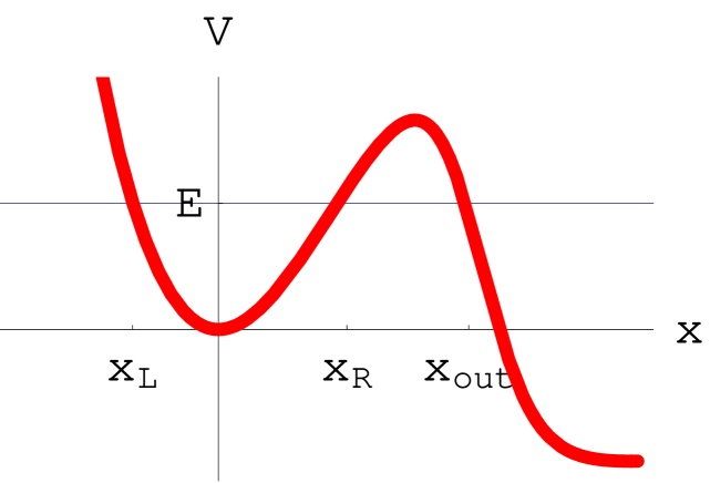
Figure 1: A schematic plot of the potential. For an energy E below the barrier there will be three classical turning points, also shown.

We begin with the simple closed quantum mechanical system formed by a particle of mass $M$ in one dimension described by a Hamiltonian

$$H=\frac{p^{2}}{2M}+U\left(x\right),$$ (1)

with a potential $U$ given by

$$U\left(x\right)=\frac{1}{2}M\Omega_{0}^{2}x^{2}-\frac{\lambda}{6}x^{3},$$ (2)

for small values of the coordinate $x$. This is a fairly general potential for a tunneling system, it is the basic element in the dashboard potential, which is a very good model for a flux trapped in a superconducting quantum interference device (SQUID), or a single Josephson junction biased by a fixed external current CalLeg83b ; MarDevCla87 ; Wei93 ; Tin96 . For technical reasons, it is convenient to assume that for large $x$ the potential flattens out and takes the value $U\left(x\right)=-U_{\infty},$ both negative and constant. The tunneling process ought to be independent of the form of the potential this far away from the potential barrier. We present a sketch of this potential in Fig. 1.

There is one classically stable point at $x=0$, and one unstable point $x=x_{s}=2M\Omega_{0}^{2}/\lambda,$  corresponding to an energy $\varepsilon_{s}=2M^{3}\Omega_{0}^{6}/(3\lambda^{2})$. The curvature of the potential is $U^{\prime\prime}(0)=M\Omega_{0}^{2}$ at $x=0,$ and $-U^{\prime\prime}(0)$  at $x_{s}.$ The other point at which $U\left(x\right)=0$ is $x=x_{exit}=(3/2)x_{s}.$ For $x\gg x_{exit}$ the potential flattens out and is constant.

II.2 The WKB approximation

If we assume that the particle is trapped in the potential well, that is in its false ground state or false vacuum, the tunneling probability can be computed in this simple problem in many ways. One of the most efficient is the instanton method which reduces to the computation of the “bounce solution”. The most attractive aspect of this computation is that it can be easily extended to field theory where the tunneling probability is then interpreted as the probability per unit time and volume to nucleate a bubble of the true vacuum phase. The rate for quantum tunneling is $\Gamma_{closed}=(\Omega_{0}/2\pi)a_{q}\exp(-S_{B}/\hbar)$, where $S_{B}$ is the action for the “bounce” (or instanton), namely the solution to the classical equations of motion which interpolates between $x=0$ and $x=x_{exit}$ in imaginary time $S_{B}=2\int_{0}^{x_{exit}}dx\;\sqrt{2MU\left(x\right)},$ and the prefactor $a_{q}=(120\pi S_{B}/\hbar)^{1/2}$. Our expression for the potential is so simple that the above integral can be computed explicitly: $S_{B}/\hbar=18\varepsilon_{s}/(5\varepsilon_{0})$, where $\varepsilon_{0}=\frac{1}{2}\hbar\Omega_{0}$ is the zero point energy of a harmonic oscillator with frequency $\Omega_{0}.$

Here, however, we will concentrate on a real time approach by expanding the false vacuum state as a linear combination of true eigenstates of the Hamiltonian. To the required accuracy, it is enough to work with the WKB approximations to the true eigenfunctions; see for instance Refs. LanLif77 ; GalPas90 . The instanton method reviewed in the previous paragraph can, in fact, be easily justified by this semiclassical approximation. Here we explain in some detail this standard procedure to obtain the eigenfunctions by matching the WKB solutions in the different regions of the potential. These solutions will play a crucial role in the energy representation for the Wigner functions to be introduced latter.

Let $0<E<\varepsilon_{s}$ be the energy of the particle in the potential well, and $\psi_{E}$ the corresponding eigenfunction. The Schrödinger equation is

$$\frac{-\hbar^{2}}{2M}\frac{\partial^{2}}{\partial x^{2}}\psi_{E}+U\left(x\right)\psi_{E}=E\psi_{E}.$$ (3)

Let us define

$$p\left(x\right)=\sqrt{2M\left|U\left(x\right)-E\right|},$$ (4)

and the integral $S(x,y)$ (note the order in the integration limits)

$$S\left(x,y\right)=\int_{y}^{x}dx^{\prime}\;p\left(x^{\prime}\right).$$ (5)

The WKB solutions are obtained from these elements. We have to match the WKB solutions in the different regions across the potential function. The details of this calculation are given in Appendix A. The WKB solution $\psi_{E}$ for energies in the range $0<E<\varepsilon_{s}$ is given by Eq. (113), where $x_{L}<x_{R}<x_{out}$ are the three classical turning points for the cubic potential (2); see Fig. 1. The normalization constant $K_{E}$ in Eq. (113) is obtained by imposing the continuous normalization of the eigenfunctions given in Eq. (115) and it is given in Eq. (122). Of particular relevance is the value of the eigenfunction $\psi_{E}(x)$ at values $x\gg x_{out}$. This gives the main contribution to the continuous normalization integral. The value of the eigenfunction at $x\gg x_{out}$, as computed in Appendix A, is

$$\psi_{E}(x)\sim\sqrt{\frac{2M}{\hbar\pi p_{\infty}}}\sin\left(\frac{p_{\infty}x}{\hbar}+\delta_{E}\right),$$ (6)

where the phase $\delta_{E}$ is introduced in Eqs. (123) and $p_{\infty}(E)$ is defined by Eq. (4) when $x\gg x_{out}$; see also Eq. (116).

We are interested in the details of the eigenfunctions near the false vacuum state, since we will be dealing with tunneling from vacuum. Thus, in the remaining of this section we give explicitly the values of the normalization constant $K_{E}$ and the phase shifts $\delta_{E}$ near this vacuum state. Therefore let us impose the Bohr-Sommerfeld quantization condition (114) and let $E_{0}$ be the corresponding lowest energy, that is, $n=0$ in Eq. (114). As we will see in the next subsection this defines the false vacuum energy. Expanding the integral in Eq. (5) around $E_{0}$ we find that close to the lowest energy value

$$S\left(x_{R},x_{L}\right)\sim\frac{\pi\hbar}{2}-\tau\left(E-E_{0}\right),$$ (7)

where $\tau$ is defined by

$$\tau=\int_{x_{L}}^{x_{R}}dx\;\sqrt{\frac{2M}{U\left(x\right)-E_{0}}}.$$ (8)

Thus $\cos^{2}\left(S\left(x_{R},x_{L}\right)/\hbar\right)\sim(\tau^{2}/\hbar^{2})\left(E-E_{0}\right)^{2}$, and evaluating the right hand side of (125) at $E_{0},$ we conclude that $K_{E}^{2}$ has poles at the complex energies

$$E_{\pm}=E_{0}\pm i\varepsilon,\qquad\varepsilon\equiv\frac{\hbar}{4\tau}e^{-2S_{0}\left(x_{out},x_{R}\right)/\hbar},$$ (9)

which is in agreement with the standard result GalPas90 . To simplify the notation let us call $S_{0}=S_{0}\left(x_{out},x_{R}\right)$ and $f_{0}=f\left(E_{0}\right)+\pi/4$, then we have from Eqs. (120) and (121) that the functions $A(E)$ and $B(E)$ for $E$ near $E_{0}$ are: $A\left(E\right)=(\tau/\hbar)\exp(S_{0}/\hbar)[F_{-}(E)+F_{+}(E)]$ and $B\left(E\right)=(-i\tau/\hbar)\exp(S_{0}/\hbar)[F_{-}(E)-F_{+}(E)]$, where $F_{-}(E)=\exp(if_{0}/\hbar)\left(E-E_{-}\right)$ and $F_{+}(E)=\exp(-if_{0}/\hbar)\left(E-E_{+}\right)$. Notice that neither $A$ nor $B$ vanish at $E_{\pm}$. Finally from Eq. (122) we can write the normalization constant near the false vacuum energy, as

$$K_{E}^{2}=\frac{M}{\pi\hbar\tau}\frac{\varepsilon}{\left(E-E_{0}\right)^{2}+\varepsilon^{2}}=\frac{4M\varepsilon^{2}}{\pi\hbar^{2}}\frac{e^{2S_{0}/\hbar}}{\left(E-E_{-}\right)\left(E-E_{+}\right)},$$ (10)

and from Eqs. (123) the phase shifts are

$$e^{i\delta_{E}}=2\sqrt{\frac{\varepsilon^{2}e^{2S_{0}/\hbar}}{\left(E-E_{0}\right)^{2}+\varepsilon^{2}}}\left(A+iB\right)=e^{if_{0}/\hbar}\sqrt{\frac{E-E_{-}}{E-E_{+}}}.$$ (11)

Equations (6), (10) and (11) are the main results of this section. We notice, in particular, the poles of the norm and the phase shifts at $E_{\pm}$ near the false vacuum energy. The strong dependence on the energy of these functions near the false ground energy will play an important role in the next sections.

II.2.1 The false vacuum

Before we start with the computation of the tunneling rate we have to define what we mean by the decaying state, all the wave functions we considered so far are true stationary states and, obviously, show no decay whatsoever. We need to confine initially the particle into the potential well in its lowest energy. To this end, we introduce an auxiliary potential $U_{\mathrm{aux}}$ which agrees with $U$ up to $x_{s}$ (where the true potential reaches its maximum value) and increases thereafter. We may assume that the growth of $U_{\mathrm{aux}}$ is as fast as necessary to justify the approximations below; the tunneling rate is insensitive to the details of $U_{\mathrm{aux}}$ beyond $x_{s}.$ Thus, we define the decaying state $\psi_{0}$ as the ground state of a particle confined by $U_{\mathrm{aux}}$ Mig77 .

It is obvious from the form of the WKB solutions that $\psi_{0}$ agrees with $\psi_{E_{0}}$ up to $x_{s}$, i. e. $\psi_{0}(x)=\psi_{E_{0}}(x)$ for $x\leq x_{s}$, where $E_{0}$ is the Bohr-Sommerfeld ground state energy for the auxiliary potential $U_{\mathrm{aux}}$, which corresponds to $n=0$ in the condition (114). Beyond $x_{s}$, $\psi_{0}$ will decay rapidly to zero, unlike $\psi_{E_{0}}.$ Like any other wave function, $\psi_{0}$ admits a development in the complete base of energy eigenfunctions $\psi_{E}$, as

$$\psi_{0}\left(x\right)=\int dE\;C_{E}\psi_{E}\left(x\right),$$ (12)

where due to our normalization the Fourier coefficients are given by

$$C_{E}=\int dx\;\psi_{E}\left(x\right)\psi_{0}\left(x\right).$$ (13)

To find these coefficients, we observe that $\psi_{0}\left(x\right)$ is a solution to the Schrödinger equation with the auxiliary potential $U_{\mathrm{aux}}$

$$\frac{-\hbar^{2}}{2M}\frac{\partial^{2}}{\partial x^{2}}\psi_{0}+U_{\mathrm{aux}}\left(x\right)\psi_{0}=E_{0}\psi_{0}.$$ (14)

Let us add to both sides of this equation the term $[U\left(x\right)-U_{\mathrm{aux}}\left(x\right)]\psi_{0}$ and then multiply both sides by $\psi_{E}\left(x\right)$ and integrate to obtain

$$\left(E-E_{0}\right)C_{E}=-\int_{x_{s}}^{\infty}dx\;\psi_{E}\left(x\right)\left[U_{\mathrm{aux}}\left(x\right)-U\left(x\right)\right]\psi_{0}\left(x\right).$$ (15)

An important consideration is that $\psi_{0}\left(x\right)$ is a smooth function (as opposed to a distribution), and, unlike $\psi_{E_{0}}$ it is normalizable, so $C_{E}$ must also be smooth. This means that it is allowable to assume $E\neq E_{0}$ in Eq. (15); $C_{E_{0}}$ can then be found by analytical continuation. To estimate the right hand side of Eq. (15), let us introduce; cf. Eq. (4),

$$p_{\mathrm{aux}}\left(x\right)=\sqrt{2M\left|U_{\mathrm{aux}}\left(x\right)-E_{0}\right|}.$$ (16)

To the right of $x_{s}$ we may use the WKB approximation with the decaying solution into the forbidden region to write

$$\psi_{0}\left(x\right)=\psi_{0}\left(x_{s}\right)e^{-\frac{1}{\hbar}\int_{x_{s}}^{x}p_{\mathrm{aux}}\left(y\right)dy}.$$ (17)

On the other hand, $\psi_{E}\left(x\right)$ is given by Eq. (111) in Appendix A. If $E$ is close to $E_{0}$, then Eq. (7) applies, and we may write

$$\psi_{E}\left(x\right)\sim 2K_{E}\left[\frac{\tau}{\hbar}\left(E-E_{0}\right)F_{+}\left(x_{s},x_{R}\right)e^{\frac{1}{\hbar}\int_{x_{s}}^{x}p\left(y\right)dy}+\frac{1}{2}F_{-}\left(x_{s},x_{R}\right)e^{-\frac{1}{\hbar}\int_{x_{s}}^{x}p\left(y\right)dy}\right].$$ (18)

Substituting the two previous expressions into the right hand side of Eq. (15) we see that we have to compute the two following integrals,

$$J_{\pm}=\int_{x_{s}}^{\infty}dx\;\left[U_{\mathrm{aux}}\left(x\right)-U\left(x\right)\right]e^{-\frac{1}{\hbar}\int_{x_{s}}^{x}\left[p_{\mathrm{aux}}\left(y\right)\pm p\left(y\right)\right]dy}.$$ (19)

The integral, $J_{-}$, is dominated by the region near the lower limit, where $p_{\mathrm{aux}}\left(x\right)$ is close to $p\left(x\right)$ and we can write

$$p_{\mathrm{aux}}\left(x\right)-p\left(x\right)\sim\frac{\left(p_{\mathrm{aux}}^{2}\left(x\right)-p^{2}\left(x\right)\right)}{2\sqrt{2MU\left(x_{s}\right)}}=\sqrt{\frac{M}{2U\left(x_{s}\right)}}\left[U_{\mathrm{aux}}\left(x\right)-U\left(x\right)+E-E_{0}\right],$$

from where we obtain

$$J_{-}=\hbar\sqrt{\frac{2U\left(x_{s}\right)}{M}}-\left(E-E_{0}\right)\int_{x_{s}}^{\infty}dx\;e^{-\frac{1}{\hbar}\int_{x_{s}}^{x}\left[p_{\mathrm{aux}}\left(y\right)-p\left(y\right)\right]dy},$$ (20)

where the remaining integral is made negligible by an appropriate choice of $U_{\mathrm{aux}}$. For the other integral, $J_{+}$, we see that the corresponding exponential factor in Eq. (19) decays faster than the exponential factor of $J_{-}$, so that the region which effectively contributes to the integral is narrower. Since the pre-exponential factor vanishes at the lower limit, we find $J_{+}\sim 0$. Finally, putting all these pieces together into the right hand side of Eq. (15) we get to leading order,

$$\left(E-E_{0}\right)\left[C_{E}+2K_{E}\psi_{0}\left(x_{s}\right)\tau\sqrt{\frac{2U\left(x_{s}\right)}{M}}F_{+}\left(x_{s},x_{R}\right)\right]=0,$$

whose solution, assumed smooth, is

$$C_{E}=-2K_{E}\psi_{0}\left(x_{s}\right)\tau\sqrt{\frac{2U\left(x_{s}\right)}{M}}F_{+}\left(x_{s},x_{R}\right).$$ (21)

We note that $C_{E}$ is independent of the choice of $U_{\mathrm{aux}}$ beyond $x_{s}$, as it should.

Thus, we have found the false vacuum wave function in terms of the energy wave functions of the original problem. The false ground state is a superposition of energy eigenstates which are fine tuned in such a way as to produce destructive interference outside the potential well. Notice that $C_{E}$, because of the factor $K_{E}$  in Eq. (21), peaks near the energy of the false ground state, and has a strong dependence on the energy near this ground state energy.

II.2.2 Tunneling from the false vacuum

Let us now compute the tunneling rate assuming that the particle is described initially by the false ground state $\psi_{0}$. At time $t$, we have

$$\psi\left(x,t\right)=\int dE\;e^{-iEt/\hbar}C_{E}\psi_{E}\left(x\right),$$ (22)

The persistence amplitude is

$$\rho\left(t\right)=\int dx\;\psi_{0}^{\ast}\left(x\right)\psi\left(x,t\right)=\int dE\;e^{-iEt/\hbar}C_{E}^{2}.$$ (23)

To perform the integration we can close the contour of integration in the complex $E$ plane adding an arc at infinity, whereby we pick up the pole $E_{-}$ in $K_{E}^{2}$; cf. Eq. (21). Therefore $\rho(t)$ goes like

$$\rho(t)\sim\exp\left[\frac{-t}{4\tau}\exp\left(-\frac{2}{\hbar}S_{0}\left(x_{out},x_{R}\right)\right)\right],$$ (24)

provided $t$ is not too large. The tunneling rate for this closed system, $\Gamma_{closed}$, may be defined from the persistence probability $\rho^{2}(t)\sim\exp(-\Gamma_{closed}t)$, so that $\Gamma_{closed}=(1/2\tau)\exp(-2S_{0}/\hbar)$, which agrees with the result of the bounce solution. Note that if we take the classical lowest energy $E=0$, then $x_{R}=x_{L}=0$, $x_{out}=x_{exit}$, and $S_{B}=2S(x_{exit},0)$, but $S_{0}$ here is the action corresponding to a particle with false vacuum energy $E_{0}$, which differs from zero, consequently it differs from $S_{B}/2$. This difference is accounted for by the prefactor $a_{q}$ in the instanton result.

An equivalent way of deriving this result is to estimate the integral by a stationary phase approximation. We can write the integral of Eq. (23) as

$$\rho(t)=\int dE\;e^{F\left[E\right]}G\left[E\right]$$

where $F\left[E\right]=-iEt/\hbar+\ln(K_{E}^{2})$ with $K_{E}^{2}$ given by (10). We consider everything else going into $G\left[E\right]$ as relatively slowly varying. The stationary phase points are the roots of $F^{\prime}=0.$ When $t\rightarrow\infty$, these roots must approach $E_{\pm}.$ Write e. g. $E=E_{-}+\varepsilon r$. If $\left|r\right|<1$, then $r=(i\hbar/\varepsilon t)[1-(\hbar/2\varepsilon t)+...]$; this approximation is consistent if $\varepsilon t/\hbar>1.$ At the stationary point

$$F\left[E\right]=-i\frac{E_{-}t}{\hbar}+\ln\left[t\right]+\mathrm{constant}.$$

The first term accounts for the exponential decay, as $E_{-}=E_{0}-i\varepsilon$ where $\varepsilon$ is given by Eq. (9), in agreement with the previous result (24). On the other hand, $F^{\prime\prime}\sim t^{2}$, so the Gaussian integral over energies contributes a prefactor of order $t^{-1}.$

III Wigner function and energy representation

A very useful description of a quantum system is that given by the Wigner function in phase space, which is defined by an integral transform of the density matrix Wig32 ; HilEtAl84 . The Wigner function for a system described by a wave function $\psi(x)$ is

$$W\left(x,p\right)=\int\frac{dy}{2\pi\hbar}\;e^{ipy/\hbar}\;\psi\left(x-\frac{y}{2}\right)\psi^{\ast}\left(x+\frac{y}{2}\right),$$ (25)

where the sign convention is chosen so that a momentum eigenstate $\psi_{p_{0}}\left(x\right)\sim e^{ip_{0}x/\hbar}/\sqrt{2\pi\hbar}$ becomes $W_{p_{0}}\left(x,p\right)=(1/2\pi\hbar)\delta\left(p-p_{0}\right)$. Moreover, it satisfies

$$\int dp\;W\left(x,p\right)=\;\left|\psi\left(x\right)\right|^{2},\qquad\int dx\;W\left(x,p\right)=\;\left|\int dx\;\frac{e^{-ipx/\hbar}}{\sqrt{2\pi\hbar}}\psi\left(x\right)\right|^{2},$$ (26)

and it is normalized so that $\int\int dx\;dp\;W(x,p)=1$. Thus the Wigner function is similar in some ways to a distribution function in phase space, it is real but, unlike a true distribution function, it is not positive defined; this is a feature connected to the quantum nature of the system it describes.

The Schrödinger equation for the wave function $\psi$,

$$\frac{-\hbar^{2}}{2M}\frac{\partial^{2}}{\partial x^{2}}\psi+U\left(x\right)\psi=i\hbar\frac{\partial}{\partial t}\psi,$$ (27)

translates into a dynamical equation for the Wigner function, which is easily derived. In fact, by taking the time derivative of (25), using the Schrödinger equation (27), and integrating by parts we have

$$\frac{\partial}{\partial t}W\left(x,p\right) = -\frac{i}{\hbar}\int\frac{dy}{2\pi\hbar}\;e^{ipy/\hbar}\;\left\{\left(\frac{-i\hbar p}{M}\right)\frac{\partial}{\partial x}\left[\psi\left(x-\frac{y}{2}\right)\psi^{*}\left(x+\frac{y}{2}\right)\right]\right.$$

$$\left.+\psi\left(x-\frac{y}{2}\right)\left[U\left(x-\frac{y}{2}\right)-U\left(x+\frac{y}{2}\right)\right]\psi^{*}\left(x+\frac{y}{2}\right)\right\}.$$

For the cubic potential (2) we have $U\left(x-y/2\right)-U\left(x+y/2\right)=-M\Omega_{0}^{2}xy+(\lambda/2)x^{2}y+(\lambda/24)y^{3}$ and, noting that $ye^{ipy/\hbar}=-i\hbar\partial_{p}e^{ipy/\hbar}$ and $y^{3}e^{ipy/\hbar}=i\hbar^{3}\partial_{p}^{3}e^{ipy/\hbar}$, we get the equation for the Wigner function

$$\frac{\partial}{\partial t}W\left(x,p\right)=\left[U^{\prime}\left(x\right)\frac{\partial}{\partial p}-\frac{p}{M}\frac{\partial}{\partial x}+\frac{\lambda}{24}\hbar^{2}\frac{\partial^{3}}{\partial p^{3}}\right]W\left(x,p\right),$$ (28)

which may be interpreted as a quantum transport equation. The first two terms on the right hand side are just the classical Liouville terms for a distribution function, the term with the three momentum derivatives is responsible for the quantum tunneling behavior of the Wigner function in our problem. A theorem by Pawula Ris89 states that a transport equation should have up to second order derivatives at most, or else an infinite Kramers-Moyal expansion, for non-negative solutions $W(x,p,t)$ to exist. The above equation for the Wigner function circumvents the implications of the theorem since it need not be everywhere-positive. Even if we have an everywhere-positive Gaussian Wigner function at the initial time, the evolution generated by an equation such as Eq. (28) will not keep it everywhere-positive. Thus, here we see the essential role played by the non-positivity of the Wigner function in a genuinely quantum aspect such as tunneling.

III.1 The energy representation

Given that a wave function $\psi$ can be represented in terms of the energy eigenfunctions $\psi_{E}$, defined by Eq. (3), as

$$\psi\left(x\right)=\int dE\;C_{E}\psi_{E}\left(x\right),$$ (29)

we can introduce a corresponding representation for $W(x,p)$ in terms of a base of functions $W_{E_{1}E_{2}}(x,p)$ in phase space defined by

$$W_{E_{1}E_{2}}\left(x,p\right)=\int\frac{dy}{2\pi\hbar}\;e^{ipy/\hbar}\;\psi_{E_{1}}\left(x-\frac{y}{2}\right)\psi_{E_{2}}^{\ast}\left(x+\frac{y}{2}\right).$$ (30)

Then $W\left(x,p\right)$ can be written as

$$W\left(x,p\right)=\int dE_{1}dE_{2}\;C_{E_{1}E_{2}}W_{E_{1}E_{2}}\left(x,p\right),$$ (31)

where, in this case, we have $C_{E_{1}E_{2}}=C_{E_{1}}C_{E_{2}}^{\ast}$. On the other hand from the definition of $W_{E_{1}E_{2}}(x,p)$ we can write

$$\int\frac{dxdp}{\hbar}W_{E_{1}E_{2}}^{*}\left(x,p\right)W_{E_{1}^{\prime}E_{2}^{\prime}}\left(x,p\right)=\int\frac{dxdy}{2\pi\hbar^{2}}\left\{\psi_{E_{1}}\left(x-\frac{y}{2}\right)\psi_{E_{2}}\left(x+\frac{y}{2}\right)\psi_{E_{1}^{\prime}}\left(x-\frac{y}{2}\right)\psi_{E_{2}^{\prime}}\left(x+\frac{y}{2}\right)\right\},$$

where the $p$ integration has been performed. If we now call $z=x-y/2$, $z^{\prime}=x+y/2$; then $dxdy=dzdz^{\prime}$, and

$$\int\frac{dxdp}{\hbar}W_{E_{1}E_{2}}^{\ast}\left(x,p\right)W_{E_{1}^{\prime}E_{2}^{\prime}}\left(x,p\right)=\frac{1}{2\pi\hbar^{2}}\delta\left(E_{1}-E_{1}^{\prime}\right)\delta\left(E_{2}-E_{2}^{\prime}\right),$$ (32)

which gives the orthogonality properties of the functions $W_{E_{1}E_{2}}$. This suggests that any Wigner function may be written in this basis as

$$W\left(x,p,t\right)=\int dE_{1}dE_{2}\;C_{E_{1}E_{2}}\left(t\right)W_{E_{1}E_{2}}\left(x,p\right).$$ (33)

We call this the energy representation of the Wigner function. In this representation, the master equation or the quantum transport equation (28) is very simple

$$\frac{\partial}{\partial t}C_{E_{1}E_{2}}\left(t\right)=\frac{-i}{\hbar}\left(E_{1}-E_{2}\right)C_{E_{1}E_{2}}\left(t\right),$$ (34)

as one can easily verify. One might give an alternative derivation of the tunneling rate from this equation, by taking the initial condition for the Wigner function which corresponds to the false vacuum. In fact, in the next section we will use the energy representation of the Wigner function to compute this rate in a more complex problem involving coupling to an environment. Note that the dynamics of the transport equation in the energy representation is trivial and the initial condition is given in terms of the coefficients (21) which we have already computed. The task would be more difficult starting from the transport equation in phase space, such as Eq. (28), since the third derivative term makes the solution of the equation very complicated. One has to resort to methods such as those based on matrix continued fractions in order to compute decay rates from master equations for open quantum systems with third order derivative terms Ris89 ; VogRis88 ; RisVog88 ; GarZue04 . We call the attention to the similarity of this representation to that based in Floquet states that one can use when the Hamiltonian is periodic Shi65 ; MilWya83 ; BluEtAl91 ; UteDitHan94 . The power of this representation will be seen in the following sections when we consider our quantum system coupled to an environment.

IV The open quantum system

So far we have considered a simple closed quantum system. From now on we will consider an open quantum system by assuming that our system of interest is coupled to an environment. As emphasized by Caldeira and Leggett CalLeg83b any quantum macroscopic system can be modelled by an open quantum system by adjusting the coupling of the system and environment variables and by choosing appropriate potentials. One of the main effects of the environment is to induce decoherence into the system which is a basic ingredient into the quantum to classical transition CalLeg83b ; Zur91 ; PazHabZur93 ; ZurPaz94 ; PazZur99 ; PazZur01 .

The standard way in which the environment is introduced is to assume that the system is weakly coupled to a continuum set of harmonic oscillators, with a certain frequency distribution. These oscillators represent degrees of freedom to which some suitable variable of the quantum system is coupled. One usually further assumes that the environment is in thermal equilibrium and that the whole system-environment is described by the direct product of the density matrices of the system and the environment at the initial time. The macroscopic quantum system is then described by the reduced density matrix, or equivalently, by the reduced Wigner function of the open quantum system. This latter function is defined from the system-environment Wigner function after integration of the environment variables.

In order to have a working model in a form as simple as possible, but that captures the main effect of the environment, we will assume that the reduced Wigner function, which we still call $W(x,p)$, satisfies the following dynamical equation,

$$\frac{\partial}{\partial t}W\left(x,p\right)=\left[U^{\prime}\left(x\right)\frac{\partial}{\partial p}-\frac{p}{M}\frac{\partial}{\partial x}+\frac{\lambda}{24}\hbar^{2}\frac{\partial^{3}}{\partial p^{3}}+\gamma\frac{\partial}{\partial p}\left(p+M\sigma^{2}\frac{\partial}{\partial p}\right)\right]W\left(x,p\right),$$ (35)

where $\gamma$ which has units of inverse time is the dissipation parameter, and $\sigma^{2}$ the diffusion coefficient. The last two terms of this equation represent the effect of the environment: the first describes the dissipation produced into the system and the second is the diffusion or noise term. An interesting limit, the so-called weak dissipation limit, is obtained when $\gamma\rightarrow 0$, so that there is no dissipation, but the diffusion coefficient $\gamma\sigma^{2}$ is kept fixed. We will generally refer to equation (35) as the quantum Kramers equation, or alternatively, as the quantum transport equation. It is worth to notice that this equation reduces to a classical Fokker-Planck transport equation when $\hbar=0$: it becomes Kramer’s equation Kra40 ; Lan69 for a statistical system coupled to a thermal bath and has the right stationary solutions.

This equation can be derived in the high temperature limit CalLeg83a ; UnrZur89 ; HuPazZha92 ; HuPazZha93 ; HalYu96 ; CalRouVer03 . In fact, assuming the so-called Ohmic distribution for the frequencies of the harmonic oscillators one obtains that, in this limit, $\sigma^{2}=k_{B}T$, where $k_{B}$ is Boltzmann’s constant and $T$ the bath temperature. In the low temperature limit, however, the master equation for the reduced Wigner function is more involved HuPazZha92 ; ArtEtAl03 . It contains time dependent coefficients and an anomalous diffusion term of the type $\nu\partial_{x}\partial_{p}\,W(x,p)$, where $\nu$ is the anomalous diffusion coefficient. Nevertheless, a good approximation to the $\sigma$ coefficient is given at zero temperature by $\sigma^{2}\sim\frac{1}{2}\hbar\Omega_{0}$. For simplicity we will base our analysis in that equation even though we are interested in quantum tunneling from vacuum which means that our quantum system is at zero temperature.

Equation (35) is often used to describe the effect of decoherence produced by the diffusion coefficient to study the emergence of classical behavior in quantum systems; this is a topic of recent interest; see Ref. PazZur01 for a review. Of particular relevance to our problem is the study of decoherence in quenched phase transitions AntLomMon01 , and the effect of decoherence in quantum tunneling in quantum chaotic systems MonPaz00 ; MonPaz01 .

The reduced Wigner function $W(x,p)$ describes the quantum state of the open quantum system, and given a dynamical variable $A(x,p)$ associated to the system its expectation value in that quantum state is defined by,

$$\left\langle A\left(x,p\right)\right\rangle=\int dxdp\;A\left(x,p\right)\;W\left(x,p\right).$$ (36)

Then one can easily prove from Eq. (35) that defining,

$$N=\int dxdp\;W\left(x,p\right),\qquad\left\langle E\right\rangle=\int dxdp\;\left(\frac{p^{2}}{2M}+U\left(x\right)\right)W\left(x,p\right),$$ (37)

we have $\dot{N}=0$ and $\langle\dot{E}\rangle=-\gamma(\langle p^{2}/M\rangle-N\sigma^{2})$.

IV.1 Energy representation of the reduced Wigner function

Let us now use the base of functions in phase space $W_{E_{1}E_{2}}(x,p)$, introduced in Eq. (30), to represent the reduced Wigner function $W\left(x,p,t\right)$ as in Eq. (33). The previous $N$ and $\left\langle E\right\rangle$ have very simple expressions in the energy representation:

$$N=\int dE\;C_{EE}\left(t\right),\qquad\left\langle E\right\rangle=\int dE\;E\;C_{EE}\left(t\right).$$ (38)

To check the last equation we note that $\int dxdp\;\left[(p^{2}/2M)+U\left(x\right)\right]W_{E_{1}E_{2}}\left(x,p\right)=E_{1}\delta\left(E_{1}-E_{2}\right),$ which can be easily proved by explicit substitution of the definition of $W_{E_{1}E_{2}}$, and trading powers of $p$ by derivatives with respect to $y$ into expressions (30), and partial integrations.

The quantum transport equation (35) in the energy representation becomes,

$$\frac{\partial}{\partial t}C_{E_{1}E_{2}}\left(t\right)=\frac{-i}{\hbar}\left(E_{1}-E_{2}\right)C_{E_{1}E_{2}}\left(t\right)+\gamma\int dE_{1}^{\prime}dE_{2}^{\prime}\;Q_{E_{1}E_{2},E_{1}^{\prime}E_{2}^{\prime}}C_{E_{1}^{\prime}E_{2}^{\prime}}\left(t\right),$$ (39)

where, after one integration by parts,

$$Q_{E_{1}E_{2},E_{1}^{\prime}E_{2}^{\prime}}=-2\pi\hbar^{2}\int\frac{dxdp}{\hbar}\left(\frac{\partial}{\partial p}W_{E_{1}E_{2}}^{*}\left(x,p\right)\right)\left(\frac{p}{M}+k_{B}T\frac{\partial}{\partial p}\right)W_{E_{1}^{\prime}E_{2}^{\prime}}\left(x,p\right),$$ (40)

which has the contributions from the dissipative and the diffusion or noise parts, respectively, as

$$Q_{E_{1}E_{2},E_{1}^{\prime}E_{2}^{\prime}}=Q_{E_{1}E_{2},E_{1}^{\prime}E_{2}^{\prime}}^{\left(D\right)}+Q_{E_{1}E_{2},E_{1}^{\prime}E_{2}^{\prime}}^{\left(N\right)}.$$ (41)

From Eq. (30) it is easy to see that these coefficients can all be written in terms of the following matrix elements:

$$X_{E_{1}E_{2}} = \int dx\;x\;\psi_{E_{1}}\left(x\right)\psi_{E_{2}}\left(x\right),$$ (42)

$$P_{E_{1}E_{2}} = \frac{\hbar}{i}\int dx\;\;\psi_{E_{1}}\left(x\right)\frac{\partial}{\partial x}\psi_{E_{2}}\left(x\right),$$ (43)

$$\left(XP\right)_{E_{1}E_{2}} = \frac{\hbar}{i}\int dx\;\;x\psi_{E_{1}}\left(x\right)\frac{\partial}{\partial x}\psi_{E_{2}}\left(x\right),$$ (44)

$$X_{E_{1}E_{2}}^{2} = \int dx\;x^{2}\;\psi_{E_{1}}\left(x\right)\psi_{E_{2}}\left(x\right).$$ (45)

Explicitly, we have that

$$Q_{E_{1}E_{2},E_{1}^{\prime}E_{2}^{\prime}}^{\left(D\right)}=\frac{-i}{2M\hbar}\left[\left(XP\right)_{E_{1}E_{1}^{\prime}}\delta\left(E_{2}-E_{2}^{\prime}\right)-P_{E_{1}E_{1}^{\prime}}X_{E_{2}E_{2}^{\prime}}-X_{E_{1}E_{1}^{\prime}}P_{E_{2}E_{2}^{\prime}}+\left(XP\right)_{E_{2}E_{2}^{\prime}}\delta\left(E_{1}-E_{1}^{\prime}\right)\right],$$ (46)

$$Q_{E_{1}E_{2},E_{1}^{\prime}E_{2}^{\prime}}^{\left(N\right)}=\frac{k_{B}T}{\hbar^{2}}\left[2X_{E_{1}E_{1}^{\prime}}X_{E_{2}E_{2}^{\prime}}-X_{E_{1}E_{1}^{\prime}}^{2}\delta\left(E_{2}-E_{2}^{\prime}\right)-X_{E_{2}E_{2}^{\prime}}^{2}\delta\left(E_{1}-E_{1}^{\prime}\right)\right].$$ (47)

Thus, in terms of the coefficients $C_{E_{1}E_{2}}$ the dynamics of the quantum transport equation is very simple. This equation, in fact, resembles a similar equation when a Floquet basis of states are used Shi65 ; MilWya83 ; BluEtAl91 ; UteDitHan94 , which are very useful when the Hamiltonian of the system is periodic in time. The Floquet basis is discrete in such a case and a numerical evaluation of the corresponding matrix elements (42)-(45) can be performed; see for instance MonPaz00 ; MonPaz01 for a recent application. It is remarkable that in our case approximated analytic expressions for these matrix elements can be found.

IV.2 Some properties of the matrix elements

The matrix elements (42)-(45) have a clear physical interpretation and several relations can be derived among them. Note that $X_{E_{1}E_{2}}$ is the matrix element of the position operator $X$ in the energy representation. Since $X\psi_{E}\left(x\right)=x\psi_{E}\left(x\right),$ we must have $\int dE_{1}\;X_{EE_{1}}\psi_{E_{1}}\left(x\right)=x\psi_{E}\left(x\right).$

On the other hand, $P_{E_{1}E_{2}}$ is the matrix element for the momentum operator. The canonical commutation relation $\left[P,X\right]=-i\hbar$, implies $\left[H,X\right]=(-i\hbar/M)P$, and taking matrix elements on both sides we have

$$\left(E_{1}-E_{2}\right)X_{E_{1}E_{2}}=-\frac{i\hbar}{M}P_{E_{1}E_{2}}.$$ (48)

Also, $X_{E_{1}E_{2}}^{2}$ is the matrix element of $X^{2}$, therefore

$$X_{E_{1}E_{2}}^{2}=\int dE\;X_{E_{1}E}X_{EE_{2}}.$$ (49)

On the other hand, $\left(XP\right)_{E_{1}E_{2}}$ is the matrix element of $XP$, consequently $\left[\left(XP\right)_{E_{2}E_{1}}\right]^{*}=-\left(XP\right)_{E_{2}E_{1}}$ corresponds to $PX$, and $\left(XP\right)_{E_{1}E_{2}}+\left(XP\right)_{E_{2}E_{1}}=\left[X,P\right]_{E_{1}E_{2}}=i\hbar\delta\left(E_{1}-E_{2}\right)$. Also $\left(XP\right)_{E_{1}E_{2}}-\left(XP\right)_{E_{2}E_{1}}=(iM/\hbar)\left(E_{1}-E_{2}\right)X_{E_{1}E_{2}}^{2}$, where the commutator $[H,X^{2}]$ has been used in the last step, therefore

$$\left(XP\right)_{E_{1}E_{2}}=\frac{iM}{2\hbar}\left(E_{1}-E_{2}\right)X_{E_{1}E_{2}}^{2}+\frac{i\hbar}{2}\delta\left(E_{1}-E_{2}\right).$$ (50)

We have, also, that $\left(XP\right)_{E_{1}E_{2}}=\int dE\;X_{E_{1}E}P_{EE_{2}}$. One may check, for consistency, that these relations imply $\dot{N}=0.$ In Appendix B a test of the quantum transport equation in the energy representation (and of the above matrix element properties) is given by checking that a stationary solution with a thermal spectrum is, indeed, a solution in the high temperature limit.

IV.3 Computing the matrix elements

The matrix elements contain singular parts coming from the integrals over the unbound region beyond $x_{s}.$ These singular parts are easy to compute, since far enough the wave functions assume the simple form (6). When performing the calculation of the singular parts of the matrix elements we will use that when $\bar{x}\rightarrow\infty$, we have the identities

$$\frac{\sin(p\bar{x}/\hbar)}{\pi p}\rightarrow\delta\left(p\right),\qquad\frac{\cos(p\bar{x}/\hbar)}{p}\rightarrow 0,$$ (51)

which can be easily checked by taking the Fourier transforms of these functions with respect to $p$.

The computation of the singular parts of the matrix elements (42)-(45) may be reduced to the evaluation of three basic integrals. These integrals are

$$A_{A,S}\left(p_{1},p_{2}\right)=\int dx\;\sin\left[\left(p_{1}\mp p_{2}\right)x/\hbar+\delta_{1}\mp\delta_{2}\right],$$ (52)

and

$$B\left(p_{1},p_{2}\right)=\int dx\;\sin\left(p_{1}x/\hbar+\delta_{1}\right)\sin\left(p_{2}x/\hbar+\delta_{2}\right),$$ (53)

where, for simplicity, we have written $p_{i}\equiv p_{\infty}\left(E_{i}\right)$ and $\delta_{i}\equiv\delta\left(E_{i}\right)$ ($i=1,2$). The matrix element $X_{E_{1}E_{2}}$ is

$$X_{E_{1}E_{2}} \sim \frac{2M}{\hbar\pi\sqrt{p_{1}p_{2}}}\int dx\;x\;\sin\left(p_{1}x/\hbar+\delta_{1}\right)\sin\left(p_{2}x/\hbar+\delta_{2}\right)$$

$$= \frac{M}{\pi\sqrt{p_{1}p_{2}}}\left[-\frac{\partial A}{\partial p_{1}}-\frac{\partial\tilde{A}}{\partial p_{2}}-\left(\frac{\partial\delta_{1}}{\partial p_{1}}+\frac{\partial\delta_{2}}{\partial p_{2}}\right)B\right],$$ (54)

where $A\equiv(A_{S}-A_{A})/2$ and $\tilde{A}\equiv(A_{S}+A_{A})/2$. The matrix element $X_{E_{1}E_{2}}^{2}$ is

$$X_{E_{1}E_{2}}^{2} \sim \frac{2M}{\hbar\pi\sqrt{p_{1}p_{2}}}\int dx\;x^{2}\;\sin\left(p_{1}x/\hbar+\delta_{1}\right)\sin\left(p_{2}x/\hbar+\delta_{2}\right)$$ (55)

$$= \frac{2M}{\pi\sqrt{p_{1}p_{2}}}\left[-\frac{\partial C}{\partial p_{1}}-\left(\frac{\partial\delta_{1}}{\partial p_{1}}\right)D\right],$$

where, it is easy to show that $C=(\partial B/\partial p_{1})-(\partial\delta_{1}/\partial p_{1})A$, and that $D=-(\partial A/\partial p_{1})-(\partial\delta_{1}/\partial p_{1})B$. The matrix element $P_{E_{1}E_{2}}$ is

$$P_{E_{1}E_{2}}\sim\frac{-iM}{\hbar\pi\sqrt{p_{1}p_{2}}}\left(p_{1}+p_{2}\right)\tilde{A},$$ (56)

which according to the relations among matrix elements derived in the previous subsection is related to $X_{E_{1}E_{2}}$ by Eq. (48). The remaining matrix element $(XP)_{E_{1}E_{2}}$, on the other hand, can be computed from the element $X_{E_{1}E_{2}}^{2}$ according to Eq. (50)

IV.3.1 The integrals $A(p_{1},p_{2})$ and $B(p_{1},p_{2})$

Thus, we are finally left with the computation of the integrals (52) and (53). The integral $B\left(p_{1},p_{2}\right)$ of Eq. (53) is dominated by its upper limit $\bar{x}$

$$B\left(p_{1},p_{2}\right) \sim \frac{1}{2}\int^{\bar{x}}dx\;\cos\left[\left(p_{1}-p_{2}\right)x/\hbar+\delta_{1}-\delta_{2}\right]$$

$$\sim \frac{1}{2\left(p_{1}-p_{2}\right)}\sin\left[\left(p_{1}-p_{2}\right)\bar{x}/\hbar+\delta_{1}-\delta_{2}\right]$$

$$\rightarrow \frac{\pi\hbar}{2}\delta\left(p_{1}-p_{2}\right),$$ (57)

The integrals $A_{A,S}\left(p_{1},p_{2}\right)$ are more subtle. The integral $A_{S}$ is clearly regular on the diagonal. Since we are interested mostly on the singular behavior of the matrix elements, we can approximate $A_{S}\sim 0.$ On the other hand $A_{A}$ is exactly zero on the diagonal. Close to the diagonal, the integral is dominated by the region where the argument of the trigonometric function is small, and thereby the integrand is non oscillatory. Estimating the upper limit of this region as $\bar{x}\sim\hbar\left(p_{1}-p_{2}\right)^{-1}$, we get

$$A_{A}\sim\hbar^{-1}\left(p_{1}-p_{2}\right)\bar{x}^{2}+\left(\delta_{1}-\delta_{2}\right)\bar{x}=\hbar PV\left(\frac{1}{p_{1}-p_{2}}\right)+...\,,$$ (58)

where the dots stand for regular terms. Actually, this argument would allow us to introduce an undetermined coefficient in front of the principal value $PV$, but in the next section we show that $\hbar$ is the correct coefficient, as follows from the canonical commutation relations.

Thus, we are now in the position to give the explicit expressions for the singular parts of the matrix elements and write, finally, the quantum transport equation in its explicit form. This is done in detail in the next section. However, there is an approximation we can use that drastically simplifies the computations, and is discussed afterwards, in subsection V.3.

V The quantum Kramers equation

In this Section we explicitly compute the quantum transport equation (35) satisfied by the reduced Wigner function in the energy representation.

V.1 Matrix elements

First, we need to compute the matrix elements described in section IV.3. We begin with the matrix element $X_{E_{1}E_{2}}$ which according to (54) and (57)-(58) can be written as:

$$X_{E_{1}E_{2}}=\frac{M\hbar}{\sqrt{p_{1}p_{2}}}\left[\frac{1}{\pi}\frac{\partial}{\partial p_{1}}PV\left(\frac{1}{p_{1}-p_{2}}\right)-\frac{\partial\delta_{1}}{\partial p_{1}}\delta\left(p_{1}-p_{2}\right)+...\right].$$ (59)

We go next to the matrix element $P_{E_{1}E_{2}}$, which from (56) and (58) can be written as,

$$P_{E_{1}E_{2}}=\frac{-iM}{\sqrt{p_{1}p_{2}}}\frac{1}{2\pi}\left(p_{1}+p_{2}\right)PV\frac{1}{p_{1}-p_{2}}.$$ (60)

These two operators $X$ and $P$ are connected through Eq. (48). It is easy to check that the two previous results satisfy this relation. Just notice that from Eq. (116) we can write $E_{1}-E_{2}=(p_{1}^{2}-p_{2}^{2})/2M$ which together with Eq. (59) for $X_{E_{1}E_{2}}$ lead to $-i\hbar/M$ times the right hand side of Eq. (60), that is

$$\left(E_{1}-E_{2}\right)X_{E_{1}E_{2}}=-\frac{i\hbar}{M}P_{E_{1}E_{2}}.$$

Another check of the previous results is the consistency with the canonical commutation relations

$$\int dE\;\left(P_{E_{1}E}X_{EE_{2}}-X_{E_{1}E}P_{EE_{2}}\right)=-i\hbar\delta\left(E_{1}-E_{2}\right).$$ (61)

This check requires a little more work. First it is convenient to change to momentum variables and write, $\delta\left(E_{1}-E_{2}\right)=(M/\sqrt{p_{1}p_{2}})\delta\left(p_{1}-p_{2}\right).$ Then one needs to compute the integral

$$I\equiv\hbar\int_{-\infty}^{\infty}dp\;PV\left(\frac{1}{p_{1}-p}\right)PV\left(\frac{1}{p-p_{2}}\right)=-\hbar\pi^{2}\delta\left(p_{1}-p_{2}\right),$$ (62)

The evaluation of this integral is easily performed using the following representation of the principal value

$$PV\left(\frac{1}{p}\right)=\int\frac{d\xi}{2\pi\hbar}\;e^{ip\xi/\hbar}\left(-i\pi\;\mathrm{sign}\left[\xi\right]\right),$$

which is easily proved by taking the Fourier transform of $PV(1/p)$. With the result of Eq. (62) it is straightforward to check that the commutation relation (61) is an identity within our approximation. This consistency check is important because it can be used to fix to $\hbar$ the coefficient in front of the principal value of $A_{A}$ in the argument leading to Eq. (58).

We can now move to the matrix elements for $X^{2}$. Having an expression for $X_{E_{1}E_{2}}$ in Eq. (59) it is best to compute $X_{E_{1}E_{2}}^{2}$ directly from the relation (49) which leads to

$$X_{E_{1}E_{2}}^{2} = \frac{M\hbar^{2}}{\sqrt{p_{1}p_{2}}}\left[\frac{\partial^{2}}{\partial p_{1}\partial p_{2}}\delta\left(p_{1}-p_{2}\right)+\frac{1}{\pi}\left(\frac{\partial\delta_{1}}{\partial p_{1}}+\frac{\partial\delta_{2}}{\partial p_{2}}\right)\frac{\partial}{\partial p_{2}}PV\left(\frac{1}{p_{1}-p_{2}}\right)\right.$$ (63)

$$\left.+\left(\frac{\partial\delta_{1}}{\partial p_{1}}\right)^{2}\delta\left(p_{1}-p_{2}\right)+...\right],$$

where we have used the result (62) and performed the $E$ integration or, more precisely, the $p$ integration.

The matrix element $(XP)_{E_{1}E_{2}}=\int dEX_{E_{1}E}P_{EE_{2}}$ can be analogously obtained from the expressions (59) and (60). The result is

$$\left(XP\right)_{E_{1}E_{2}}=\frac{iM\hbar}{2\sqrt{p_{1}p_{2}}}\left[2p_{2}\frac{\partial}{\partial p_{1}}\delta\left(p_{1}-p_{2}\right)+\frac{1}{\pi}\frac{\partial\delta_{1}}{\partial p_{1}}\left(p_{1}+p_{2}\right)PV\left(\frac{1}{p_{1}-p_{2}}\right)+...\right].$$ (64)

A further consistency check of these expressions comes from the property (50), which is satisfied within our approximation.

V.2 The quantum transport equation

Finally, we can write the quantum transport equation in the energy representation (39) with the coefficient $Q$ given by (41). The values of the dissipative and noise parts are given, respectively, by (46) and (47), which can be directly computed using the matrix elements deduced in the previous subsection. It is convenient to define,

$$C_{E_{1}E_{2}}\left(t\right)=\frac{1}{\sqrt{p_{1}p_{2}}}C_{p_{1}p_{2}}\left(t\right),$$ (65)

and the result is the rather cumbersome expression (130) given in Appendix C. As explained there we can get a local approximation of the quantum transport equation (130), namely

$$\frac{\partial C_{p_{1}p_{2}}}{\partial t} = \frac{-i}{2M\hbar}(p_{1}^{2}-p_{2}^{2})C_{p_{1}p_{2}}+\frac{\gamma}{2}\left(\frac{\partial}{\partial p_{1}}+\frac{\partial}{\partial p_{2}}\right)\left[\left(p_{1}+p_{2}\right)C_{p_{1}p_{2}}\right]$$ (66)

$$+\gamma M\sigma^{2}\left[\left(\frac{\partial}{\partial p_{1}}+\frac{\partial}{\partial p_{2}}\right)^{2}-\left(\frac{\partial\delta_{1}}{\partial p_{1}}-\frac{\partial\delta_{2}}{\partial p_{2}}\right)^{2}\right]C_{p_{1}p_{2}}.$$

It is suggestive to give interpretations to the last three terms in this quantum Kramers equation. The first, of course, is the dissipation term, whereas the second and third are diffusion terms. The first involves the dissipation coefficient, that defines a time scale $\tau_{R}\sim\gamma^{-1}$, which is the relaxation time.

Before we go on with the interpretation of the different terms, it is important to recall the meaning of the coefficients $C_{p_{1}p_{2}}$, or $C_{E_{1}E_{2}}$. First, we note that these coefficients are directly related to the coefficients $C_{E}$ of the energy eigenfunctions which make the tunneling state from the false vacuum in the isolated system, i. e. when there is no interaction to the environment. Thus, the coefficients $C_{E_{1}E_{2}}$ clearly give the quantum correlations between wave functions of different energies that make the tunneling system. These coefficients are initially separable $C_{E_{1}E_{2}}(0)=C_{E_{1}}(0)C_{E_{2}}^{\ast}(0)$. In the isolated closed system its time evolution, as given by Eq. (34), is simply $C_{E_{1}E_{2}}(t)=C_{E_{1}E_{2}}(0)\exp[-i(E_{1}-E_{2})t/\hbar]$, which means that these correlations keep their amplitude in its dynamical evolution.

This is very different in the open quantum system. The negative last term in Eq. (66) has no effect when $E_{1}=E_{2}$, i. e. for the diagonal coefficients, but its effect is very important for the off-diagonal coefficients. In fact, the amplitude of the off-diagonal coefficients exponentially decays in time, on a time scale of the order of

$$\tau_{D}\sim\tau_{R}\left(\frac{\lambda_{B}}{l_{D}}\right)^{2},$$ (67)

where $\tau_{R}$ is the relaxation time, $\lambda_{B}=\hbar/(2\sigma\sqrt{M})$ is a characteristic de Brolie wavelength (in the high temperature case when $\sigma^{2}=k_{B}T$ it corresponds to the thermal de Broglie wavelength), and $l_{D}\sim\alpha^{2}\hbar\sqrt{E_{0}+U_{\infty}}/(\varepsilon\sqrt{M})$ is a characteristic length of the problem with $\alpha$ a dimensionless parameter that measures the scale of the energy differences of the off-diagonal coefficient, $E_{1}-E_{2}\sim\alpha\varepsilon$; so it is of order 1 when the energy differences are of order $\varepsilon$. The time scale (67) can be estimated by taking the derivatives of the phase shifts $\delta_{i}$ ($i=1,2$) near the false vacuum energy $E_{0}$, which is where the energy wavefunctions pile up. Thus, the last term of equation (66) destroys the quantum correlations of the energy eigenfunctions. The time scale $\tau_{D}$ may be considered as a decoherence time Zur91 , and thus the effect on tunneling of this term may be associated to the effect of decoherence.

Another time scale in the problem is, of course, the tuneling time which according to (24) and (9) is given by $\tau_{\mathrm{tunn}}\sim\hbar/\varepsilon$. Its relation to $\tau_{D}$ is given by $\tau_{D}\sim\tau_{\mathrm{tunn}}/(\alpha^{4}D)$, where the dimensionless parameter $D$ is defined in (77).

The last of the diffusion terms is the only one that survives in the phase shift approximation which we introduce in the next subsection. This is justified by the strong dependence of the phase shifts $\delta_{i}$, ($i=1,2$) on the energy near the vacuum energy, see Eq. (11), which make the derivatives of these functions very large near $E_{0}$. Note also that the range of energies (and momenta) in Eq. (66) is also limited to near $E_{0}$ as the coefficients $C_{E}$ that describe the tunneling state are peaked there; cf. Eq. (21).

V.3 The phase shift approximation

The phase shift approximation is based on the observation made in Section II.2 that the phase shifts are fast varying functions of energy near resonance. This suggests: (a) we only keep the singular terms, and of these, (b) only those which contain derivatives of the phase shifts. Under this approximation we can go back to Eqs. (54)-(56) to write,

$$X_{E_{1}E_{2}}\sim\frac{-\hbar M}{p_{1}}\left(\frac{\partial\delta_{1}}{\partial p_{1}}\right)\delta\left(p_{1}-p_{2}\right),$$ (68)

$$X_{E_{1}E_{2}}^{2}\sim\frac{\hbar^{2}M}{\sqrt{p_{1}p_{2}}}\left(\frac{\partial\delta_{1}}{\partial p_{1}}\right)^{2}\delta\left(p_{1}-p_{2}\right),$$ (69)

moreover $P_{E_{1}E_{2}}\sim 0$, and $(XP)_{E_{1}E_{2}}\sim 0$. Now we see from (46) that $Q_{E_{1}E_{2},E_{1}^{\prime}E_{2}^{\prime}}^{\left(D\right)}\sim 0$, so that only the diffusion term $Q_{E_{1}E_{2},E_{1}^{\prime}E_{2}^{\prime}}^{\left(N\right)}$ matters, and this term is proportional to $\delta\left(E_{1}-E_{1}^{\prime}\right)\delta\left(E_{2}-E_{2}^{\prime}\right)$ (we change from variables $p_{i}$ to $E_{i}$ according to $p_{i}dp_{i}=MdE_{i}$). This means that we are working in a weak dissipation limit. Finally, the quantum transport equation (39) can be written as

$$\frac{\partial}{\partial t}C_{E_{1}E_{2}}\left(t\right)=-L\left[E_{1},E_{2}\right]C_{E_{1}E_{2}}\left(t\right),$$ (70)

where

$$L\left[E_{1},E_{2}\right]=\frac{i}{\hbar}\left(E_{1}-E_{2}\right)+\frac{\gamma\sigma^{2}}{M}\left(p_{1}\frac{\partial\delta_{1}}{\partial E_{1}}-p_{2}\frac{\partial\delta_{2}}{\partial E_{2}}\right)^{2}.$$

This equation, of course, can also be obtained from Eq. (66) in the limit where only the phase shift terms of the environment are kept and we return to the $E_{i}$ variables instead of the $p_{i}$. In the spirit of the phase shift approximation, we shall replace $p_{i}$ ($i=1,2$) by their values at resonance, whereby

$$L\left[E_{1},E_{2}\right]=\frac{i}{\hbar}\left(E_{1}-E_{2}\right)+2\gamma\sigma^{2}(E_{0}+U_{\infty})\left(\frac{\partial\delta_{1}}{\partial E_{1}}-\frac{\partial\delta_{2}}{\partial E_{2}}\right)^{2},$$ (71)

where, from Eq. (11), the phase shifts derivatives are

$$\frac{\partial\delta}{\partial E}=\frac{-i}{2}\left(\frac{1}{E-E_{-}}-\frac{1}{E-E_{+}}\right).$$ (72)

VI Tunneling in the open quantum system

We can now compute the tunneling rate from the false vacuum for our open quantum system. Thus, let us assume that our particle at $t=0$ is trapped into the well of the potential (2) in the false ground state with the energy $E_{0}$, i. e. the ground state of the auxiliary potential $U_{\mathrm{aux}}$ introduced in Section II.2.1. We know from that section that the wave function $\psi_{0}$ of this state can be expressed in terms of the eigenfunctions $\psi_{E}$ by Eq. (12) with the coefficients $C_{E}$ given by Eq. (21). In terms of the reduced Wigner function, which we may call $W_{0}(x,p)$, this state is easily described in the energy representation (33) by the coefficients $C_{E_{1}E_{2}}(0)=C_{E_{1}}(0)C_{E_{2}}^{*}(0)$, where $C_{E}(0)$ is just given by Eq. (21). Because the dynamics of the quantum transport equation is trivial in the energy representation (70) the time dependence of the coefficients $C_{E_{1}E_{2}}(t)$ is simply

$$C_{E_{1}E_{2}}\left(t\right)=\exp\left(-L\left[E_{1},E_{2}\right]t\right)C_{E_{1}E_{2}}\left(0\right),$$ (73)

so that, according to Eq. (33), the Wigner function at any time is

$$W\left(x,p,t\right)=\int dE_{1}dE_{2}\;\exp\left(-L\left[E_{1},E_{2}\right]t\right)C_{E_{1}}\left(0\right)C_{E_{2}}\left(0\right)W_{E_{1}E_{2}}\left(x,p\right).$$ (74)

From this we can compute, in particular, the probability of finding the particle at the false vacuum at any time. In terms of the false vacuum Wigner function and the Wigner function of the tunneling system we may define that probability as

$$\rho^{2}(t)=2\pi\hbar\int dx\,dp\,W_{0}(x,p)W(x,p,t).$$ (75)

This equation is justified by observing that in the closed system of Section II where the state is described by the wave function $\psi$ of Eq. (22) and the false vacuum is described by the wave function $\psi_{0}$ of Eq. (12), the square of the persistence amplitude (23) is given, in fact, by Eq. (75) when the definition of the Wigner function , i. e. Eq. (25), is used. For the open system the quantum state is not described by a pure state and, in general, the Wigner function $W(x,p,t)$ can be written as $W=\sum_{i}p_{i}W_{i}$ where $p_{i}$ is the probability of finding the system in the state $\phi_{i}$ and $W_{i}$ is the Wigner function for the state $\phi_{i}$. The definition (75) leads in this case to $\rho^{2}(t)=\sum_{i}p_{i}|\langle\psi_{0}|\phi_{i}\rangle|^{2}$, which is indeed the probability of finding the system in the state $\psi_{0}$. Eq. (75) when the energy representation (33) is used becomes

$$\rho^{2}\left(t\right)=\int dE_{1}dE_{2}\;\exp\left(-L\left[E_{1},E_{2}\right]t\right)C_{E_{1}}^{2}\left(0\right)C_{E_{2}}^{2}\left(0\right).$$ (76)

To compute $\rho^{2}\left(t\right)$ we shall use the stationary phase approximation. The idea is that the integration paths for $E_{1}$ and $E_{2}$ may be deformed simultaneously in such a way that the integrand comes to be dominated by Gaussian peaks. For late times it is enough to seek the stationary points of $L\left[E_{1},E_{2}\right].$ In principle, we could include $K_{E_{1}}^{2}$ and $K_{E_{2}}^{2}$ as fast varying components of the integrand, but these functions are really fast varying in the vicinity of $E_{-}$ and $E_{+},$ which, when $\gamma\neq 0$, are essential singularities of the integrand and must be avoided. Note that when deforming the path of integration, we should avoid regions where Re $L<0$. Then, calling

$$E_{i}=E_{0}+\varepsilon r_{i}\ \ \ (i=1,2),\qquad D=\gamma\hbar\sigma^{2}\frac{(E_{0}+U_{\infty})}{\varepsilon^{3}},$$ (77)

where $\varepsilon$ was introduced in Eq. (9), and using Eq. (72) for the phase shift derivatives we find that

$$L\left[E_{1},E_{2}\right]t=\frac{t\varepsilon}{\hbar}\left[i\left(r_{1}-r_{2}\right)+2D\left(\frac{1}{1+r_{1}^{2}}-\frac{1}{1+r_{2}^{2}}\right)^{2}\right].$$ (78)

The stationary phase condition, $dL/dE_{1}=0$ and $dL/dE_{2}=0$, reads

$$f_{1}\left[r_{1},r_{2}\right]\equiv i-8D\left(\frac{1}{1+r_{1}^{2}}-\frac{1}{1+r_{2}^{2}}\right)\frac{r_{1}}{\left(1+r_{1}^{2}\right)^{2}}=0,$$ (79)

and there is a similar equation $f_{2}\left[r_{1},r_{2}\right]=0$, where $f_{2}\left[r_{1},r_{2}\right]$ is obtained from $f_{1}\left[r_{1},r_{2}\right]$, with the substitution of the multiplying factor $r_{1}/\left(1+r_{1}^{2}\right)^{2}$ by $r_{2}/\left(1+r_{2}^{2}\right)^{2}$. Observe that $f_{2}\left[r_{1},r_{2}\right]=-\left(f_{1}\left[r_{2}^{*},r_{1}^{*}\right]\right)^{*}$, so a solution of Eq. (79) with $r_{2}=r_{1}^{*}$ is automatically also a solution of $f_{2}\left[r_{1},r_{2}\right]=0$. We shall seek stationary points of this kind. It is clear that for a solution of this kind, $r_{1}/\left(1+r_{1}^{2}\right)^{2}$ must be real. So, writing $r_{1}=\xi-i\eta$, we must have $4\xi^{2}\left(1+\xi^{2}\right)=\left(1+\xi^{2}-\eta^{2}\right)^{2}$, and solving for $\xi^{2}$ we find

$$3\xi^{2}=\left[\left(2-\eta^{2}\right)^{2}+3\eta^{4}\right]^{1/2}-1-\eta^{2}.$$ (80)

We notice that for each value of $\eta$ there will be two possible solutions for $\xi$. The path of integration must go through both of them. Substituting, $r_{1}=\xi-i\eta$, into the complex stationary phase equation (79) we obtain two equations for $\xi$ and $\eta$. The real part of Eq. (79) leads to the previous Eq. (80), which is independent of $D$, and the imaginary part leads to

$$32D\xi^{2}\eta\left[\left(1+\xi^{2}-\eta^{2}\right)^{2}+4\eta^{2}\left(1-\eta^{2}\right)\right]=\left[\left(1+\xi^{2}-\eta^{2}\right)^{2}+4\xi^{2}\eta^{2}\right]^{3}.$$ (81)

For each value of $D$, we are interested in the solutions with the lowest possible positive value of $\eta$.

Finally, the contribution of each saddle point to the integral will be

$$\rho_{\pm}^{2}(t)=\Delta_{\pm}e^{-tL\left[\pm\xi,\eta\right]},$$ (82)

where

$$L\left[\pm\xi,\eta\right]=\frac{2\varepsilon\eta}{\hbar}\left(1-16D\xi^{2}\eta\left[\left(1+\xi^{2}-\eta^{2}\right)^{2}+4\xi^{2}\eta^{2}\right]^{-2}\right),$$

and where the prefactor $\Delta_{\pm}$ depends on the second derivatives of $L$. Comparing to the persistence probability $\rho_{\mathrm{closed}}^{2}\sim\exp\left(-2t\varepsilon/\hbar\right)$ for the isolated closed quantum system, which follows from the persistence amplitude Eq. (24) and the definition of $\varepsilon$ given in Eq. (9), we conclude that the ratio $R=\Gamma_{open}/\Gamma_{closed}$ of the tunneling rates between the open, $\Gamma_{open}=L$, and closed, $\Gamma_{closed}=2\varepsilon/\hbar$, systems is

$$R=\eta\left(1-16D\xi^{2}\eta\left[\left(1+\xi^{2}-\eta^{2}\right)^{2}+4\xi^{2}\eta^{2}\right]^{-2}\right),$$ (83)

where the parametres $\xi$ and $\eta$ are solutions of the algebraic equations (80) and (81) with the lowest possible positive value of $\eta$.

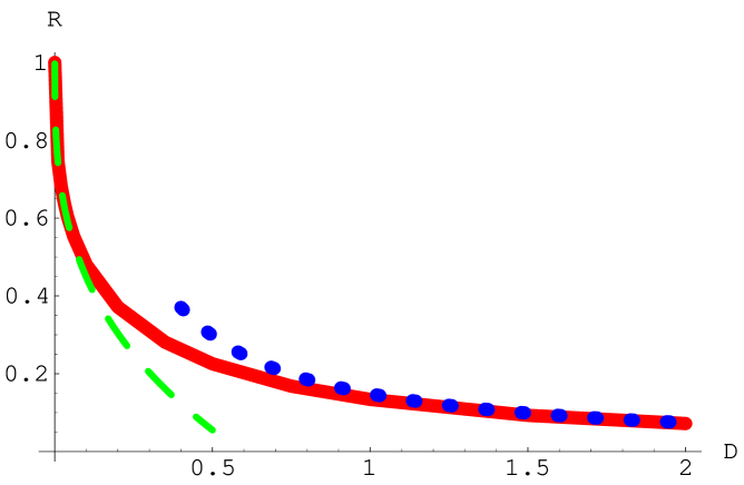
Figure 2: The ratio $R$ between the tunneling rates for the open system and the closed system as a function of the dimensionless parameter $D$ (full line). We also plot the analytic approximations for low and large values of $D$ (dashed and dotted lines, respectively).

In Fig. 2 we plot $R$ as a function of $D$ from a numerical solution of Eqs. (81) and (80) (full line); we see that $R<1$ for all values of $D,$ with tunneling being strongly suppressed when $D$ is large. In the asymptotic limits $D\rightarrow 0$ and $D\rightarrow\infty$ it is possible to obtain analytical approximations. In the former, $\eta=1-\delta,$ $\xi=\pm\delta,$ where $\delta=\left(D/2\right)^{1/3}.$ In this limit

$$R_{D\rightarrow 0}\sim 1-\frac{3}{2}\left(\frac{D}{2}\right)^{1/3},$$ (84)

which is also plotted in Fig. 2 (dashed line). In the opposite limit, $D\rightarrow\infty,$ we have $\eta=8/\left(27D\right),$ $\xi=\pm 1/\sqrt{3}$ and

$$R_{D\rightarrow\infty}\sim\frac{4}{27D},$$ (85)

which is plotted in Fig. 2 (dotted line).

Observe that if we included the factors of $K_{E_{i}}^{2}$ ($i=1,2$) into the fast varying part of the integral, then the saddle points shift by an amount $\sim\hbar/(\varepsilon t)$; therefore these results are reliable when $(\varepsilon t/\hbar)D^{1/3}\gg 1.$ On the other hand, when $\varepsilon t/\hbar$ is extremely large, the energy integrals are dominated by the contribution from the lower limit $-U_{\infty}$ and the decay rate turns to a power law.

VII Comparing with experiment

In this section we confront with experimental results. One of the experiments in which macroscopic quantum tunneling has been observed in more detail is a single Josephson junction between two superconducting electrodes biased by an external current. The macroscopic variable in this case is the phase difference $\varphi$ of the Cooper pair wave function across the junction CalLeg83b . A macroscopic system always interacts with an environment and a physical Josephson junction is generally described by an ideal one shunted by a resistance and a capacitance which phenomenologically account for the effects of the environment.

The basic equations relate the (gauge invariant) phase difference $\varphi,$ the current $I$ and the voltage $V$ across an ideal junction Tin96 ; MarDevCla87 . A zero voltage supercurrent $I=I_{c}\sin\varphi,$ should flow between two superconducting electrodes separated by a thin insulating barrier, where $I_{c}$ is the critical current, the maximum supercurrent the junction can support. If a voltage difference $V$ is maintained across the junction the phase difference evolves according to $2eV=\hbar d\varphi/dt$, where $2e$ is the charge of a Cooper pair, and $\hbar/(2e)$ is the flux quantum. It is convenient to introduce the characteristic energy scale $E_{J}=\hbar I_{c}/2e$; note that the work necessary to raise the phase difference across the ideal junction from $0$ to $\varphi$ is $\left(-E_{J}\right)\cos\varphi$. A real junction is modelled as an ideal one in parallel with an ordinary resistance $R_{\Omega}$, which build in dissipation in the finite voltage regime, and an ordinary capacitance $C$, which reflects the geometric shunting capacitance between the two superconducting electrodes. The so-called bias current flowing through the device is $I=I_{c}\sin\varphi+V/R_{\Omega}+CdV/dt$, and substituting the previous relationship between $V$ and $d\varphi/dt$, this equation becomes a differential equation for the phase difference of the Cooper pair $\varphi$:

$$M\left(\frac{d^{2}\varphi}{dt^{2}}+\gamma\frac{d\varphi}{dt}\right)+\tilde{U}^{\prime}\left(\varphi\right)=0,$$ (86)

which has the form of the equation of motion for a particle in a one-dimensional potential with friction. We have introduced the “mass” $M=\hbar^{2}C/(2e)^{2}$, the friction coefficient $\gamma=1/(R_{\Omega}C)$, and the “potential”

$$\tilde{U}\left(\varphi\right)=\left(-E_{J}\right)\left(\cos\varphi+s\varphi\right),$$ (87)

where $s\equiv I/I_{c}$. This is the so-called “tilted washboard” model. Note that when $s=1$ the local minima of the tilted cosine become inflection points, and that no classical stable equilibrium points exist when $s\geq 1$. We will be interested in the case in which $s$ is smaller but close to $1$, that is when the external biased current $I$ is slightly less than the critical current $I_{c}$.

In this case, the potential may be approximated by a cubic potential in the neighborhood of any stable stationary point. Let us consider the stable stationary point closest to $\varphi=0.$ The stationarity condition is $\sin\varphi=s$ and the stability condition is $\cos\varphi>0$. We see that there must be a solution $\varphi_{0}\leq\pi/2$, thus let us write $\varphi_{0}=\frac{\pi}{2}-\kappa$, where $\kappa\sim\sqrt{2\left(1-s\right)}\sim\sqrt{1-s^{2}}$. We henceforth introduce a new variable $x=\varphi-\varphi_{0}$ and the shifted potential

$$U\left(x\right)=\tilde{U}\left(\varphi_{0}+x\right)-\tilde{U}\left(\varphi_{0}\right),$$ (88)

which leads to the same equation (86) than the potential (87). In the new variable, the stable stationary point lies at $x=0.$ The closest unstable stationary point, the maximum of the potential lies at $x_{s}=2\kappa$, and following the notation of Sec. II, we have that the height of the potential barrier has an energy $\varepsilon_{s}\equiv U\left(x_{s}\right)$, given by

$$\varepsilon_{s}\sim\frac{2}{3}E_{J}\left[2\left(1-s\right)\right]^{3/2}\sim\frac{2}{3}E_{J}\left(1-s^{2}\right)^{3/2}.$$ (89)

Finally, the next root of the potential is $x_{exit},$ where $\tilde{U}\left(\varphi_{0}+x_{exit}\right)=\tilde{U}\left(\varphi_{0}\right)$, which can be approximately written as $sx_{exit}-\sin(x_{exit}-\kappa)\sim\kappa.$ Observe that $x_{exit}\sim 3\kappa\sim\left(3/2\right)x_{s},$ which is similar to what happens with the cubic potential of Sec. II. Note that when $s$ is nearly $1$ the height of the potential barrier $\varepsilon_{s}$ is much less than the potential difference between adjacent wells and the potential can be approximated by a cubic potential. For $\left|x\right|$ no much larger than $x_{exit},$ we may approximate $U\left(x\right)\sim\varepsilon_{s}(x/x_{s})^{2}(1-x/x_{exit})/(1-x_{s}/x_{exit})$, from where we may define the frequency $\Omega_{0}$ of small oscillations around $x=0$: $M\Omega_{0}^{2}=U^{\prime\prime}(0)$, which gives

$$\Omega_{0}^{2}\sim\frac{3\varepsilon_{s}}{2\left(1-s^{2}\right)M}\sim\frac{4e^{2}E_{J}}{\hbar^{2}C}\left(1-s^{2}\right)^{1/2}\equiv\omega_{p}^{2},$$ (90)

where $\omega_{p}$ is the “plasma frequency” of the junction. We may introduce $\omega_{p0}\equiv(4e^{2}E_{J}/\hbar^{2}C)^{1/2}=(2eI_{c}/\hbar C)^{1/2}.$

In the literature there are several reported observations of tunneling in this or more complex set-ups DevMarCla85 ; MarDevCla87 ; CleMarCla88 ; WalEtAl03 ; FulDun74 ; SchEtAl85 ; SilLieGra88 ; Sil92 ; LiEtAl02 ; MonMygRiv02 ; MonMygRiv03 ; FisWalUst03 . From this wealth of data we have chosen to focus on comparison against the experiments reported in Ref. CleMarCla88 . In that paper, tunneling was observed under a fixed bias current, as opposed to a time-dependent one FulDun74 . The fixed current environment is closest to the ideal situation to which our model applies.

A critical input in comparing theory to observations is the value of the critical current for the junction. In Ref. CleMarCla88 the critical current is not derived from the tunneling rate itself, as advocated in Ref. GraOlsWei86 , but extracted from an independent set of measurements at high temperature. We therefore find that the comparison of theory and experiment may be done in two ways: it is possible to derive the escape temperature from the independently measured critical current, as it is done in Ref. CleMarCla88 , or else it is possible to induce the value of the critical current from the observed rate. This value may then be compared to the one obtained in high temperature determinations. In the following we present both analysis.

VII.1 Tunneling rates for the open system

Let us first compare our theoretical model against the value for the tunneling amplitude (extrapolated up to) at $T=0,$ as reported in Ref. CleMarCla88 . The relevant values for the bias current $I$, the critical current $I_{c}$, its ratio $s$, the self-capacitance $C$, and shunt resistance $R_{\Omega}$ are:

$$I\sim 24.710\;\mu\mathrm{A},\ I_{c}\sim 24.873\;\mu\mathrm{A},\ s\sim 0.9934,\ C\sim 4.28\;\mathrm{pF},\ R_{\Omega}\sim 9.3\;\mathrm{\Omega}.$$ (91)

These parameters were measured in the classical limit. In previous similar experiments on current-biased junctions but with low dissipation DevMarCla85 ; MarDevCla87 it was shown that at low temperature the tunneling rate became almost independent of temperature.

Since $\hbar=1.054572\times 10^{-34}\;\mathrm{Js}$ and $e=1.602176\times 10^{-19}\;\mathrm{C}$ we have, in the conditions of Ref. CleMarCla88 , $E_{J}\sim 8.185\times 10^{-21}\;\mathrm{J}$, which using Boltzmann’s constant $k_{B}=1.380650\times 10^{-23}\;\mathrm{JK}^{-1},$ may be converted into a temperature $E_{J}/k_{B}\sim 592.9\;\mathrm{K}.$ Therefore the height of the barrier $\varepsilon_{s}$, $\omega_{p0}$, the plasma frequency $\Omega_{0}$, the zero point energy $\varepsilon_{0}=\frac{1}{2}\hbar\Omega_{0}$, and the friction coefficient $\gamma$ in our model are:

$$\varepsilon_{s}/k_{B}\sim 589.74\;\mathrm{mK},\ \omega_{p0}\sim 132.88\times 10^{9}\;\mathrm{s}^{-1},\ \Omega_{0}\sim 44.918\times 10^{9}\;\mathrm{s}^{-1},\$$

$$\varepsilon_{0}/k_{B}\sim 171.55\;\mathrm{mK},\ \gamma\sim 25.123\times 10^{9}\;\mathrm{s}^{-1}.$$ (92)

We observe that the zero point energy is lower than the barrier, although not much lower. In fact, there is only one trapped excited state.

It is often convenient to give tunneling rates in terms of an effective escape temperature $T_{esc}$. This escape temperature is defined MarDevCla87 from a given tunneling rate, $\Gamma$, by the equation

$$\Gamma\equiv\frac{1}{2\tau}e^{-\varepsilon_{s}/k_{B}T_{esc}}.$$ (93)

For the closed system, either the WKB approximation or the instanton method yield $T_{esc}\sim 71\;\mathrm{mK,}$ with a barrier penetrability $\Lambda$, defined by $\Gamma_{closed}=(1/2\tau)\exp(-\Lambda)$ (which gives $\Lambda=(2/\hbar)S_{0}$ in the WKB approximation), of $\Lambda=8.459$; see Eq. (137) in Appendix D.

For the open system, the tunneling rate in our model may be expressed in terms of $R$, introduced in Eq. (83) as the ratio between the open and closed systems rates, namely

$$\Gamma_{open}=R\,\Gamma_{closed}=\frac{R}{2\tau}e^{-\Lambda}.$$ (94)

The relevant parameter in $R$ is $D$ which was introduced in (77), where at zero temperature $\sigma^{2}\sim\varepsilon_{0}$ and also $\varepsilon_{0}\sim E_{0}$. Thus we have $D=16\pi^{3}(\gamma/\Omega_{0})(1+U_{\infty}/E_{0})\exp(3\Lambda)$. With the numerical values given in (91)-(92), $D$ is very large and we are in the limit of Eq. (85), namely $R\sim 4/(27D)$. Comparing Eq. (94) with Eq. (93), and assuming $U_{\infty}/E_{0}<1$, we may find our predicted effective escape temperature from $\varepsilon_{s}/(k_{B}T_{esc})\sim\Lambda+\ln(27D/4)\sim 4\Lambda+8.\,827$, which leads to $T_{esc}\sim 14.\,255\;\mathrm{mK}.$

The experimental result CleMarCla88 when extrapolated to the zero temperature limit is, in terms of the effective escape temperature, $T_{esc,exp}\sim 45\;\mathrm{mK}$. The experimental result is in good agreement with the instanton prediction of Caldeira and Leggett for weak dissipation at zero temperature CalLeg83b ; see also GraWei84 ; HanTalBor90 ; Wei93 . Our prediction goes in the sense that dissipation also suppresses tunneling but the predicted value for the effective escape temperature is lower than the observed result. We recall that our prediction is based on Eq. (70) which was derived under an approximation that fully neglects any activation that would increase the effective escape temperature. A better approximation based on Eq. (66) would require a numerical solution, but our starting phenomenological equation (35) is too crude to expect a quantitative agreement with the experimental result at very low temperatures at the level of accuracy of the experiment.

VII.2 The critical current

The value of the critical current is a crucial input in the calculation of the tunneling rate GraOlsWei86 . We are primarily interested in the tunneling rate under fixed bias current. However, the critical current was not determined under these conditions, but extracted from the average of measurements of tunneling rates under a ramped bias current performed at several different temperatures. For this reason, it is meaningful to contrast theory and experiment in a different way than in the previous subsection, namely, instead of computing the tunneling rate from the given values of the critical and bias currents, we may instead compute the critical current from the given bias current and tunneling rate. We may then see if the critical current obtained this way is consistent from that obtained from the ramped current measurements also reported in Ref. CleMarCla88 .

Recalling that the relation between the critical and bias currents is $I_{c}=I/s$, where we will now assume that $s$ is so far unknown but close to unity, we may write $E_{J}=\hbar I/(2es)$. Then, from (89) we have that the height of the potential barrier in terms of the parameter $s$ is, $\varepsilon_{s}\sim(\hbar I/3e)s^{-1}(1-s^{2})^{3/2}$, and from (90) the frequency of small oscillations is $\Omega_{0}\sim(2eI/\hbar C)^{1/2}s^{-1/2}(1-s^{2})^{1/4}.$ We shall assume that the ground state energy is close to the zero point energy $E_{0}\sim\varepsilon_{0}=\hbar\Omega_{0}/2$. The ratio of the ground state energy to the height of the barrier is thus, in terms of $s$,

$$\frac{E_{0}}{\varepsilon_{s}}\sim\frac{\bar{\rho}\,s^{1/2}}{(1-s^{2})^{5/4}},$$ (95)

where $\bar{\rho}\equiv(9e^{3}/2\hbar CI)^{1/2}\sim 1.288\times 10^{-3}.$

As we discuss in Appendix D, due to the form of the potential the action under the barrier, $S(x_{out},x_{R})$, for the energy $E$ is equal to the action inside the barrier, $S(x_{R},x_{L})$, for an energy $E_{ref}=\varepsilon_{s}-E.$ Writing as in Eq. (134) $E_{ref}=2\varepsilon_{s}\zeta\left(k_{ref}\right)$, where $\zeta(k)$ is defined in Eq. (135), we get $(1-s^{2})^{5/4}s^{-1/2}=\bar{\rho}[1-2\zeta\left(k_{ref}\right)]^{-1/2},$ which relates the parameter $s$ with $k_{ref}$. The corresponding penetrability, defined here as $\Lambda=(2/\hbar)S(x_{out},x_{R})$, is

$$\Lambda=\frac{27}{8}\frac{F\left(k_{ref}\right)}{1-2\zeta\left(k_{ref}\right)},$$ (96)

where $F\left(k_{ref}\right)$ is defined in Eq. (136). The tunneling rate according to Eq. (94) is then

$$\Gamma_{open}=\frac{\Omega_{0}^{2}}{2\pi\gamma}\frac{4}{27\times 16\times\pi^{3}}e^{-4\Lambda}.$$ (97)

We must compare this with the experimental tunneling rate which may be computed from Eq. (93) with the effective escape temperature $T_{esc,exp}\sim 45\;\mathrm{mK}$, and with the barrier hight $\varepsilon_{s}$ computed with a critical current $I_{c}\sim 24.873\;\mu\mathrm{A}$. Finally, equating the tunneling rate (97) with the experimental one, using the relevant numerical values given previously, we get

$$\frac{4F\left(k_{ref}\right)}{1-2\zeta\left(k_{ref}\right)}-\frac{2}{5}\ln\left[\frac{1}{1-2\zeta\left(k_{ref}\right)}\right]=5.075+\frac{4}{5}\ln\left(\frac{1}{s}\right).$$ (98)

This equation must be solved simultaneously with the previous equation relating $s$ with $k_{ref}$. The solution is $k_{ref}\sim 0.1162$ and $s\sim 0.9968.$ Thus the critical current is

$$I_{c}\sim 24.789\;\mu\mathrm{A}.$$ (99)

Observe that our model neglects any contribution that leads to activation, and therefore underestimates the tunneling rate MarGra88 . In matching against experiment, this effect is compensated by lowering the predicted critical current. Therefore this result must be regarded as a lower bound. With this in mind, the agreement with the value of $I_{c}\sim 24.873\;\mu\mathrm{A}$ extracted from the ramped current measurements CleMarCla88 is satisfactory.

VIII Conclusions

To conclude, let us briefly summarize our findings. We have computed analytically the effect of decoherence on quantum tunneling in a model representing a quantum particle, trapped in a local minimum of a potential, which is coupled to an environment characterized by a dissipative and a diffusion parameter. We have used the master equation for the reduced Wigner function, or quantum transport equation, that describes this open quantum system.

Our computational method involves the introduction of an energy representation of the reduced Wigner function which is based on the energy eigenfunctions of the isolated system. The dynamical equation in this representation, Eq. (39), is an equation for some coefficients that describe the quantum correlations between eigenfunctions of different energies. The equation can be explicitly written in a local approximation, the quantum transport equation (66), that captures the essential physics of the problem.

In our problem, where the particle is initially trapped in the false vacuum, the transport equation is dominated by a term that destroys the quantum correlations of the eigenfunctions and is, thus, responsible for decoherence. The strength of this term is characterized by the dimensionless parameter $D$, defined in Eq. (77), which is directly proportional to the energy difference between the false and true vacuum. It does not seem surprising that decoherence suppresses tunneling, as it destroys the fine tuning among the energy eigenfunctions that makes tunneling possible in the isolated closed system. The analytic result for the ratio of the tunneling rates between the open and isolated closed systems is given by Eq. (83). This ratio decreases, implying more suppression, with increasing $D$.

Our model is based in the phenomenological transport equation (35) for the reduced Wigner function, which is a toy model at zero temperature. Besides this assumption, in the paper we work at two different levels of approximation. We first derive Eq. (66), which still retains the leading effects of noise, dissipation and decoherence. To be able to isolate the effects of decoherence, we then proceed to derive the simpler Eq. (70). The actual predictions for tunneling rates are obtained from this later equation, which in practice means to pick up the environment terms that give the most decoherence, and presumably the most tunneling suppression. This means that we have neglected from the remaining terms any activation that would increase the effective escape temperature. Therefore the results from our model, derived from Eq. (70), must be regarded as a lower bound on the actual rates. This is consistent with our goal, which is not to provide an alternative to the instanton calculations in equilibrium, but to propose a starting point for a real time formulation of nonequilibrium macroscopic quantum tunneling. When seen under this light, it is encouraging that the detailed matching against experimental results shows that our model not only captures the main effect, since indeed the measured rate is substantially lower than the quantum prediction for the closed system, but also yields a suitable estimate of the critical current from the given tunneling rate. One might try to improve on this prediction by numerically solving the quantum Kramers equation (66), on which we expect to report in a separate publication. The extent of the discrepancy can be seen also as a check on the validity of the phenomenological terms introduced into the master equation for the reduced Wigner function at low temperature.

One should note that our approximations are valid when the initial state is the false vacuum. The results might differ, even qualitatively, when more general initial conditions are assumed and the terms that we have neglected in the quantum transport equation become relevant. It may not be possible in such a case to solve analytically the quantum transport equation. Yet, we should emphasize that this equation in the energy representation is much simpler than in the standard phase space representation.

Appendix A WKB solution

In this Appendix we solve the WKB problem posed in section II.2. The starting point are Eqs. (3), (4) and (5) with the cubic potential of Eq. (2), we have to match the WKB solutions in the different regions across the potential function.

A.1 Matching from forbidden to allowed regions

Let $x_{0}$ be a classical turning point $U\left(x_{0}\right)=E,$ and let $U^{\prime}\left(x_{0}\right)<0.$ Then to the left of $x_{0}$ we have a forbidden region, the two corresponding independent WKB solutions of the Schrödinger equation (3) are

$$F_{\pm}\left(x_{0},x\right)=\frac{e^{\pm S\left(x_{0},x\right)/\hbar}}{\sqrt{2p\left(x\right)/\hbar}},$$ (100)

whereas to the right of $x_{0}$ the two independent solutions are

$$G_{\pm}\left(x,x_{0}\right)=\frac{e^{\pm iS\left(x,x_{0}\right)/\hbar}}{\sqrt{2p\left(x\right)/\hbar}},$$ (101)

and we wish to find the corresponding matching conditions. For $x\rightarrow x_{0}^{-},$ we can Taylor expand the potential around $x_{0}$ and write $p\left(x\right)=\kappa\left(x_{0}-x\right)^{1/2}$ and $S\left(x_{0},x\right)=\frac{2}{3}\kappa\left(x_{0}-x\right)^{3/2}$, where we have introduced $\kappa=\sqrt{2M\left|U^{\prime}\left(x_{0}\right)\right|}$. Similarly for $x\rightarrow x_{0}^{+},$ we have $p\left(x\right)=\kappa\left(x-x_{0}\right)^{1/2}$ and $S\left(x,x_{0}\right)=\frac{2}{3}\kappa\left(x-x_{0}\right)^{3/2}.$

If we write $x-x_{0}=e^{i\pi}\left(x_{0}-x\right)$ then $iS\left(x,x_{0}\right)=S\left(x_{0},x\right)$ and it would seem that simple analytical continuation yields $G_{+}\left(x,x_{0}\right)\rightarrow e^{-i\pi/4}F_{+}\left(x_{0},x\right)$. However, this is impossible, recall that if we define the flux $J=-i(\psi^{\ast}\partial_{x}\psi-\psi\partial_{x}\psi^{\ast})$ then the Schrödinger equation implies flux conservation $\partial_{x}J=0$. Now $G_{+}\left(x,x_{0}\right)$ has $J=1$ and therefore it cannot turn into $F_{+}\left(x_{0},x\right),$ which is real, and has $J=0$. Thus, we try instead

$$G_{+}\left(x,x_{0}\right)\rightarrow e^{-i\pi/4}F_{+}\left(x_{0},x\right)+\beta F_{-}\left(x_{0},x\right),$$ (102)

and imposing flux conservation we obtain $\beta=(1/2)\exp(i\pi/4)$. We therefore find the matching conditions

$$e^{\mp i\pi/4}F_{+}\left(x_{0},x\right)+\frac{1}{2}e^{\pm i\pi/4}F_{-}\left(x_{0},x\right)\rightarrow G_{\pm}\left(x,x_{0}\right),$$ (103)

from were we finally obtain, using Eq. (101),

$$F_{+}\left(x_{0},x\right)\rightarrow\frac{1}{\sqrt{2p\left(x\right)/\hbar}}\cos\left(\frac{1}{\hbar}S\left(x,x_{0}\right)+\frac{\pi}{4}\right),$$ (104)

and

$$F_{-}\left(x_{0},x\right)\rightarrow\frac{2}{\sqrt{2p\left(x\right)/\hbar}}\sin\left(\frac{1}{\hbar}S\left(x,x_{0}\right)+\frac{\pi}{4}\right).$$ (105)

A.2 Matching from allowed to forbidden regions

Now consider the case when $U^{\prime}\left(x_{0}\right)>0.$ To the left of $x_{0},$ we have an allowed region and the solutions are oscillatory $G_{\pm}\left(x_{0},x\right)$, to the right of the turning point we have a forbidden region and the solutions are a linear combination of (100). By exactly the same procedure of the previous section, after imposing flux conservation across $x_{0}$ we obtain:

$$G_{\mp}\left(x_{0},x\right)\rightarrow e^{\pm i\pi/4}F_{+}\left(x,x_{0}\right)+\frac{1}{2}e^{\mp i\pi/4}F_{-}\left(x,x_{0}\right).$$ (106)

Note from these equations that the solution that matches a decreasing exponential is

$$\frac{1}{\sqrt{2p\left(x\right)/\hbar}}\sin\left(\frac{1}{\hbar}S\left(x_{0},x\right)+\frac{\pi}{4}\right)\rightarrow\frac{1}{2}F_{-}\left(x,x_{0}\right).$$ (107)

A.3 WKB solution for $0<E<\varepsilon_{s}$

We can now put all this together to write the energy eigenfunctions for our cubic potential (2) for energies in the range $0<E<\varepsilon_{s}$. There are three classical turning points in this case $x_{L}<x_{R}<x_{out}.$ To the left of $x_{L}$ we have a forbidden zone extending to $-\infty,$ so we have

$$\psi_{E}\left(x\right)\sim K_{E}F_{-}\left(x_{L},x\right);\qquad x<x_{L},$$ (108)

where $K_{E}$ is a normalization constant to be determined latter. To the right of $x_{L}$ we have from (105)

$$\psi_{E}\left(x\right)\sim\frac{2K_{E}}{\sqrt{2p\left(x\right)/\hbar}}\sin\left(\frac{1}{\hbar}S\left(x,x_{L}\right)+\frac{\pi}{4}\right),$$ (109)

which after using the definition (5) can be rewritten in the region $x_{L}<x<x_{R}$ as

$$\psi_{E}\left(x\right)\sim K_{E}\left(e^{i\left(S\left(x_{R},x_{L}\right)/\hbar-\pi/4\right)}G_{-}\left(x_{R},x\right)+e^{-i\left(S\left(x_{R},x_{L}\right)/\hbar-\pi/4\right)}G_{+}\left(x_{R},x\right)\right).$$ (110)

This expression is in the form suitable for extension to the forbidden region, that is, to the right of $x_{R}$. Thus, by using (106) we have to the right of $x_{R}$

$$\psi_{E}\left(x\right)\sim 2K_{E}\left[\cos\left(\frac{1}{\hbar}S\left(x_{R},x_{L}\right)\right)F_{+}\left(x,x_{R}\right)+\frac{1}{2}\sin\left(\frac{1}{\hbar}S\left(x_{R},x_{L}\right)\right)F_{-}\left(x,x_{R}\right)\right],$$ (111)

which can be rewritten again as

$$\psi_{E}\left(x\right)\sim 2K_{E}\left[\cos\left(\frac{1}{\hbar}S\left(x_{R},x_{L}\right)\right)e^{S\left(x_{out},x_{R}\right)/\hbar}F_{-}\left(x_{out},x\right)+\frac{1}{2}\sin\left(\frac{1}{\hbar}S\left(x_{R},x_{L}\right)\right)e^{-S\left(x_{out},x_{R}\right)/\hbar}F_{+}\left(x_{out},x\right)\right],$$ (112)

which is in a form suitable for extension to the right of $x_{out}$:

$$\psi_{E}\left(x\right) \sim \frac{2K_{E}}{\sqrt{2p\left(x\right)/\hbar}}\left[2\cos\left(\frac{1}{\hbar}S\left(x_{R},x_{L}\right)\right)e^{S\left(x_{out},x_{R}\right)/\hbar}\sin\left(\frac{1}{\hbar}S\left(x,x_{out}\right)+\frac{\pi}{4}\right)\right.$$ (113)

$$\left.+\frac{1}{2}\sin\left(\frac{1}{\hbar}S\left(x_{R},x_{L}\right)\right)e^{-S\left(x_{out},x_{R}\right)/\hbar}\cos\left(\frac{1}{\hbar}S\left(x,x_{out}\right)+\frac{\pi}{4}\right)\right].$$

Note that if we impose the Bohr-Sommerfeld quantization rule

$$S\left(x_{R},x_{L}\right)=\frac{\pi}{2}(1+2n)\hbar,$$ (114)

only the subdominant, exponential decreasing part survives. This would correspond to the case when the far right region is forbidden and may be used to define energies for false states trapped into the potential well, in particular $n=0$ will correspond to the false ground state.

A.4 Normalization

All that remains now is the determination of the normalization constant $K_{E}$ which can be done from the normalization of the wave functions. The eigenfunctions are subject to continuous normalization

$$\int dx\;\psi_{E_{1}}\left(x\right)\psi_{E_{2}}\left(x\right)=\delta\left(E_{1}-E_{2}\right).$$ (115)

Since the functions themselves are regular, the singular behavior must come from the upper limit, see for instance LanLif77 . For large enough $x,$ we have from Eq. (5)

$$p\rightarrow p_{\infty}=\sqrt{2M\left(E+U_{\infty}\right)}.$$ (116)

Let us write from Eq. (100),

$$S\left(x,x_{out}\right)=p_{\infty}\left(x-x_{out}\right)+\int_{x_{out}}^{x}dx^{\prime}\;\left[\sqrt{2M\left(E-U\left(x^{\prime}\right)\right)}-\sqrt{2M\left(E+U_{\infty}\right)}\right],$$ (117)

if this integral converges, we may take the upper limit of integration to $\infty,$ whereby

$$S\left(x,x_{out}\right)=p_{\infty}x+f\left(E\right),$$ (118)

where $f(E)$ stands for the second term of (117). Then, for $x\gg x_{out}$, we can write from (113) and (118)

$$\psi_{E}\left(x\right)\sim\frac{\sqrt{2\hbar}K_{E}}{\sqrt{p_{\infty}}}\left[A\left(E\right)\sin\left(\frac{p_{\infty}x}{\hbar}\right)+B\left(E\right)\cos\left(\frac{p_{\infty}x}{\hbar}\right)\right],$$ (119)

where $A(E)$ and $B(E)$ are given by

$$A\left(E\right) = 2\cos\left(\frac{1}{\hbar}S\left(x_{R},x_{L}\right)\right)e^{S\left(x_{out},x_{R}\right)/\hbar}\cos\left(f\left(E\right)+\frac{\pi}{4}\right)$$ (120)

$$-\frac{1}{2}\sin\left(\frac{1}{\hbar}S\left(x_{R},x_{L}\right)\right)e^{-S\left(x_{out},x_{R}\right)/\hbar}\sin\left(f\left(E\right)+\frac{\pi}{4}\right),$$

$$B\left(E\right) = 2\cos\left(\frac{1}{\hbar}S\left(x_{R},x_{L}\right)\right)e^{S\left(x_{out},x_{R}\right)/\hbar}\sin\left(f\left(E\right)+\frac{\pi}{4}\right)$$ (121)

$$+\frac{1}{2}\sin\left(\frac{1}{\hbar}S\left(x_{R},x_{L}\right)\right)e^{-S\left(x_{out},x_{R}\right)/\hbar}\cos\left(f\left(E\right)+\frac{\pi}{4}\right).$$

Substituting Eq. (119) into (115), the singular terms in the normalization integral are

$$\int dx\;\psi_{E_{1}}\left(x\right)\psi_{E_{2}}\left(x\right)\sim\hbar^{2}\pi\frac{K_{E_{1}}^{2}}{p_{1}}\left[A^{2}\left(E_{1}\right)+B^{2}\left(E_{1}\right)\right]\left[\frac{dp_{1}}{dE_{1}}\right]^{-1}\delta\left(E_{1}-E_{2}\right),$$

where the delta function comes from the $x$ integration which brings $\delta(p_{1}-p_{2})$ and where we have defined $p_{i}\equiv p_{\infty}(E_{i})$ ($i=1,2$) and changed from momentum to energy variables according to $p_{i}dp_{i}=MdE_{i}$; see Eq. (116). The normalization condition reduces to $1$ the coefficient of the delta function above

$$\hbar^{2}\pi\frac{K_{E_{1}}^{2}}{M}\left[A^{2}\left(E_{1}\right)+B^{2}\left(E_{1}\right)\right]=1.$$ (122)

This suggests the introduction of the phase $\delta_{E}$ as follows,

$$K_{E}A\left(E\right)=\sqrt{\frac{M}{\hbar^{2}\pi}}\cos\delta_{E},\qquad K_{E}B\left(E\right)=\sqrt{\frac{M}{\hbar^{2}\pi}}\sin\delta_{E}.$$ (123)

Thus, the eigenfunction at $x\gg x_{out}$ is Eq. (6), that is

$$\psi_{E}\left(x\right)\sim\sqrt{\frac{2M}{\hbar\pi p_{\infty}}}\sin\left(\frac{p_{\infty}x}{\hbar}+\delta_{E}\right).$$

To work out the constant $K_{E}$ in greater detail we note that form Eqs. (120) and (121) we have

$$A^{2}+B^{2}=4\cos^{2}\left(\frac{1}{\hbar}S\left(x_{R},x_{L}\right)\right)e^{2S\left(x_{out},x_{R}\right)/\hbar}+\frac{1}{4}\sin^{2}\left(\frac{1}{\hbar}S\left(x_{R},x_{L}\right)\right)e^{-2S\left(x_{out},x_{R}\right)/\hbar},$$ (124)

which is non vanishing as long as $E$ is real. However, if we allow for complex energies, as is typical of unstable states, it may be zero provided

$$\cos^{2}\left(\frac{1}{\hbar}S\left(x_{R},x_{L}\right)\right)=\frac{-1}{16}\sin^{2}\left(\frac{1}{\hbar}S\left(x_{R},x_{L}\right)\right)e^{-4S\left(x_{out},x_{R}\right)/\hbar}.$$ (125)

The left hand side is zero whenever the energy satisfies the Bohr-Sommerfeld condition (114).

Appendix B Thermal spectrum

In this Appendix we check that the quantum transport equation (39) admits a stationary solution with a thermal spectrum. This can be seen as a test on the restrictions satisfied by the matrix elements (42)-(45) with $\sigma^{2}=k_{B}T$.

An unnormalized thermal density matrix in the position representation reads,

$$\rho\left(x,x^{\prime}\right)=\int dE\;e^{-\beta E}\psi_{E}\left(x\right)\psi_{E}\left(x^{\prime}\right),$$ (126)

where $\beta=(k_{B}T)^{-1}$ and its associated Wigner function is

$$W_{\beta}\left(x,p\right)=\int dE\;e^{-\beta E}W_{EE}\left(x,p\right),$$ (127)

which in the energy representation in the base $W_{E_{1}E_{2}}$ of Eq. (33) corresponds to the coefficients $C_{E_{1}E_{2}}=e^{-\beta E_{1}}\delta\left(E_{1}-E_{2}\right)$. Inserting this into the transport equation we get

$$\int dE\;e^{-\beta E}Q_{E_{1}E_{2},EE}=0,$$ (128)

which after using Eqs. (41), (46) and (47) can be written in operator language as

$$0 = \frac{1}{2M}\frac{i}{\hbar}\left(XPe^{-\beta H}-e^{-\beta H}PX-Pe^{-\beta H}X+Xe^{-\beta H}P\right)$$

$$+\frac{1}{\beta\hbar^{2}}\left(X^{2}e^{-\beta H}+e^{-\beta H}X^{2}-2Xe^{-\beta H}X\right).$$

At the infinite temperature limit, $\beta=0,$ this is

$$0=\frac{1}{M}\frac{i}{\hbar}\left(XP-PX\right)-\frac{1}{\hbar^{2}}\left(X^{2}H+HX^{2}-2XHX\right).$$ (129)

The first term is the commutator which gives $-M^{-1}$, and the second term can be written as $-\frac{1}{\hbar^{2}}\left[X,\left[X,H\right]\right]$, which using $\left[H,X\right]=(\hbar/i)(P/M)$ is easily seen to cancel the first term.

Appendix C Quantum transport equation

Here we write explicitly the quantum transport equation (39) in the energy representation. The coefficient $Q$ in Eq. (39) is given by (41), and the values of the dissipative and noise parts of this coefficient are given, respectively, by Eqs. (46) and (47). These parts can be directly written using the matrix elements deduced in Section V. When the coefficients $C_{p_{1}p_{2}}$ defined in Eq. (65) are introduced the transport equation becomes,

$$\frac{\partial C_{p_{1}p_{2}}}{\partial t} = \frac{-i}{2M\hbar}(p_{1}^{2}-p_{2}^{2})C_{p_{1}p_{2}}+\frac{\gamma}{2}\left(\frac{\partial}{\partial p_{1}}+\frac{\partial}{\partial p_{2}}\right)\left[(p_{1}+p_{2})C_{p_{1}p_{2}}\right]$$ (130)

$$+\frac{\gamma}{4\pi^{2}}\frac{\partial}{\partial p_{1}}\int dp_{1}^{\prime}dp_{2}^{\prime}\;\left(p_{2}+p_{2}^{\prime}\right)P(p_{2}-p_{2}^{\prime})P(p_{1}-p_{1}^{\prime})C_{p_{1}^{\prime}p_{2}^{\prime}}$$

$$+\frac{\gamma}{4\pi^{2}}\frac{\partial}{\partial p_{2}}\int dp_{1}^{\prime}dp_{2}^{\prime}\;\left(p_{1}+p_{1}^{\prime}\right)P(p_{2}-p_{2}^{\prime})P(p_{1}-p_{1}^{\prime})C_{p_{1}^{\prime}p_{2}^{\prime}}$$

$$+\frac{\gamma}{4\pi}\left(\frac{\partial\delta_{1}}{\partial p_{1}}-\frac{\partial\delta_{2}}{\partial p_{2}}\right)\int dp\;\left[\left(p_{1}+p\right)P(p_{1}-p)C_{pp_{2}}-\left(p_{2}+p\right)P(p_{2}-p)C_{p_{1}p}\right]$$

$$+\gamma M\sigma^{2}\left[\frac{\partial^{2}}{\partial p_{1}^{2}}+\frac{\partial^{2}}{\partial p_{2}^{2}}-\left(\frac{\partial\delta_{1}}{\partial p_{1}}-\frac{\partial\delta_{2}}{\partial p_{2}}\right)^{2}\right]C_{p_{1}p_{2}}$$

$$+\gamma M\sigma^{2}\int dp_{1}^{\prime}dp_{2}^{\prime}\frac{2}{\pi^{2}}\frac{\partial P\left(p_{1}-p_{1}^{\prime}\right)}{\partial p_{1}}\frac{\partial P\left(p_{2}-p_{2}^{\prime}\right)}{\partial p_{2}}C_{p_{1}^{\prime}p_{2}^{\prime}}$$

$$+\gamma M\sigma^{2}\int\frac{dp_{2}^{\prime}}{\pi}\left(\frac{\partial\delta_{2}}{\partial p_{2}}+\frac{\partial\delta_{2^{\prime}}}{\partial p_{2}^{\prime}}-2\frac{\partial\delta_{1}}{\partial p_{1}}\right)\frac{\partial P(p_{2}-p_{2}^{\prime})}{\partial p_{2}}C_{p_{1}p_{2}^{\prime}}$$

$$+\gamma M\sigma^{2}\int\frac{dp_{1}^{\prime}}{\pi}\left(\frac{\partial\delta_{1}}{\partial p_{1}}+\frac{\partial\delta_{1^{\prime}}}{\partial p_{1}^{\prime}}-2\frac{\partial\delta_{2}}{\partial p_{2}}\right)\frac{\partial P(p_{1}-p_{1}^{\prime})}{\partial p_{1}}C_{p_{1}^{\prime}p_{2}},$$

where we have used the shorthand notation $P(x)\equiv PV(1/x)$.

This equation simplifies considerably if we assume that $C_{p_{1}p_{2}}\sim C\left(p_{1}\right)\delta\left(p_{1}-p_{2}\right)$, with $C\left(p\right)$ slowly varying. This is justified by noticing the effect of the second local $\sigma^{2}$ term which is negative. This term has no effect on the diagonal terms, when $p_{1}=p_{2}$, but its effect on the off-diagonal coefficients is very important. In fact, it exponentially reduces the coefficients $C_{p_{1}p_{2}}$ on a time scale of the decoherence time, as discussed in Section V. One may argue that since tunneling is a long time process with a typical scale of time $\tau_{\mathrm{tunn}}\sim\hbar/\varepsilon$ the local approximation should give a reasonable approximation to the transport equation (66) whenever $\tau_{D}\ll\tau_{\mathrm{tunn}}$.

Now, from Eq. (62) and the diagonality assumption for the $C_{p_{1}p_{2}}$ coefficients we have that

$$\int dp_{1}^{\prime}dp_{2}^{\prime}\frac{1}{\pi^{2}}\frac{\partial P\left(p_{1}-p_{1}^{\prime}\right)}{\partial p_{1}}\frac{\partial P\left(p_{2}-p_{2}^{\prime}\right)}{\partial p_{2}}C_{p_{1}^{\prime}p_{2}^{\prime}}=\frac{\partial^{2}}{\partial p_{1}\partial p_{2}}C_{p_{1}p_{2}}.$$

This term together with the two local terms involving second order derivatives of the momenta in Eq. (130) become

$$\gamma M\sigma^{2}\left(\frac{\partial}{\partial p_{1}}+\frac{\partial}{\partial p_{2}}\right)^{2}C_{p_{1}p_{2}},$$

from where Eq. (66) follows as the local approximation of the quantum transport equation (130).

Appendix D Tunneling rates for the closed system

In this Appendix we review the calculation of the quantum mechanical tunneling rate for the closed system, that is, ignoring the interaction with the environment. The quantum tunneling rate as given by the instanton calculation CalLeg83b ; GraWei84 ; MarDevCla87 is

$$\Gamma_{closed}^{(inst)}=\frac{a_{q}}{2\tau}e^{-\Lambda_{0}},$$ (131)

where $\tau=\pi/\Omega_{0}$, $\Lambda_{0}=S_{B}/\hbar=18\varepsilon_{s}/(5\varepsilon_{0})\sim 12.\,\allowbreak 376$, and the prefactor $a_{q}=(120\pi\Lambda_{0})^{1/2}\sim 68.306$ . With these values, the escape temperature defined in Eq. (93) is

$$T_{esc}^{(inst)}=\frac{\varepsilon_{0}/k_{B}}{3.6-(\varepsilon_{0}/\varepsilon_{s})\ln a_{q}}\sim 72.345\;\mathrm{mK}.$$ (132)

It is interesting to check that this result agrees with the result we obtain when the dissipation is zero. We can use our WKB result as obtained in Sec. II, see Eq. (24), to write

$$\Gamma_{closed}^{(WKB)}=\frac{1}{2\tau}e^{-\Lambda},$$ (133)

where $\Lambda=(2/\hbar)S_{0}(x_{out},x_{R})$, with $S_{0}$ defined in Eqs. (4)-(5), where the potential $U(x)$ is given by Eq. (88).

For a cubic potential, the relationship among the energy $E,$ the frequency $\Omega$ and the action $S\left(x_{R},x_{L}\right)$ is best given in parametric form,

$$E=2\varepsilon_{s}\zeta\left(k\right),\quad\Omega=\Omega_{0}f\left(k\right),\quad S\left(x_{R},x_{L}\right)=\frac{\varepsilon_{s}}{\Omega_{0}}F\left(k\right),$$ (134)

with $0<k<1$, and

$$\zeta\left(k\right)=\frac{1}{8}\left\{2+3\frac{\left(1+k^{2}\right)}{\left[Q\left(k\right)\right]^{1/2}}-\frac{\left(1+k^{2}\right)^{3}}{\left[Q\left(k\right)\right]^{3/2}}\right\},$$ (135)

$$f\left(k\right)=\left\{\frac{2}{\pi}\left[4Q\left(k\right)\right]^{1/4}K\left[k^{2}\right]\right\}^{-1},$$

$$F\left(k\right)=\frac{27}{8}\left[\frac{4}{Q\left(k\right)}\right]^{5/4}\left\{a\left(k\right)E\left[k^{2}\right]-\left(1-k^{2}\right)b\left(k\right)K\left[k^{2}\right]\right\},$$ (136)

where $E\left[k^{2}\right]$ and $K\left[k^{2}\right]$ are the complete elliptic integrals, and we have introduced the functions $Q\left(k\right)=(1/4)\left(1+14k^{2}+k^{4}\right),$ $a\left(k\right)=(16/15)\left(2-k^{2}\right)^{2}-(1/5)\left(1-k^{2}\right)\left(21-5k^{2}\right)$ and $b\left(k\right)=(8/15)\left(2-k^{2}\right)-\left(1-k^{2}\right).$

The Bohr-Sommerfeld condition Eq. (114) for the ground state ($n=0$), corresponds to the parameter $k_{GS}$ such that $F\left(k_{GS}\right)=\pi\varepsilon_{0}/\varepsilon_{s}$ which implies that $k_{GS}\sim 0.1152$. This corresponds to $\zeta\left(k_{GS}\right)\sim 0.1423$ and $f\left(k_{GS}\right)\sim 0.9550,$ while the harmonic approximation for the potential yields $0.1454$ and $1$, respectively.

To compute the barrier penetrability, $\Lambda=(2/\hbar)S_{0}(x_{out},x_{R})$, we observe that $S\left(x_{out},x_{R}\right)$ at energy $E$ is equal to $S\left(x_{R},x_{L}\right)$ at energy $E_{ref}=\varepsilon_{s}-E.$ The exchange of $E$ by $E_{ref}$ is equivalent to the exchange of $k$ by $k_{ref},$ where $\zeta\left(k_{ref}\right)=1/2-\zeta\left(k\right).$ For $k_{GS}$ we obtain $k_{ref}\sim 0.2433$ and $F\left(k_{ref}\right)\sim 2.4073$. Therefore

$$\Lambda=\frac{\varepsilon_{s}}{\varepsilon_{0}}F\left(k_{ref}\right)\sim 8.459.$$ (137)

This is to be compared against the instanton exponent $\Lambda_{0}-\ln a_{q}\sim 8.152.$ In terms of the escape temperature, the WKB approximation yields

$$T_{esc}^{(WKB)}=\frac{\varepsilon_{0}/k_{B}}{F\left(k_{ref}\right)-(\varepsilon_{0}/\varepsilon_{s})\ln\left(\Omega_{GS}/\Omega_{0}\right)}\sim 70.869\;\mathrm{mK},$$ (138)

which is in good agreement with the instanton result. This, of course, should not be surprising since for a closed system our method reduces to the standard WKB calculation. The purpose of this exercise is just to check the consistency of our calculation and to illustrate how the instanton and WKB methods compare. That the difference between $\exp(\Lambda_{0})$ and $\exp(\Lambda)$ is accounted for by the prefactor $a_{q}$ of Eq. (131) can be seen analytically by a perturbative calculation.

References

- (1) A.O. Caldeira and A.J. Leggett, Ann. Phys. 149, 374 (1983).
- (2) M. H. Devoret, J. M. Martinis and J. Clarke, Phys. Rev. Lett. 55, 1908 (1985).
- (3) J. M. Martinis, M. H. Devoret, and J. Clarke, Phys. Rev. B 35, 4682 (1987).
- (4) A. N. Cleland, J. M. Martinis and J. Clarke, Phys. Rev. B 37, 5950 (1988).
- (5) A. Wallraff, T. Duty, A. Lukashenko, and A. V. Ustinov, Phys. Rev. Lett, 90, 037003 (2003).
- (6) A.O. Caldeira and A.J. Leggett, Phys. Rev. Lett. 46, 211 (1981).
- (7) A.J. Leggett, S. Chakravarty, A. T. Dorsey, M. P. A. Fisher, A. Garg and W. Zwerger, Rev. Mod. Phys. 59, 1 (1987).
- (8) P. Hänggi, Ann. N. Y. Acad. Sci. 480, 51 (1986).
- (9) P. Hänggi, Z. Phys. B 68, 181 (1987).
- (10) U. Weiss, H. Grabert, P. Hänggi and P. S. Riseborough, Phys. Rev. B 35, 9535 (1987).
- (11) H. P. Grabert, P. Olschowski and U. Weiss, Phys. Rev. B 36, 1931 (1987).
- (12) H. Grabert, U. Weiss and P. Hänggi, Phys. Rev. Lett. 52, 2193 (1984).
- (13) U. Griff, H. Grabert, P. Hänggi, and P. S. Riseborough, Phys. Rev. B 40, 7295 (1989).
- (14) J. M. Martinis and H. Grabert, Phys. Rev. B 38, 2371 (1988).
- (15) H. Grabert and U. Weiss, Phys. Rev. Lett. 53, 1787 (1984).
- (16) U. Weiss, Quantum Dissipative Systems (World Scientific, Singapore, 1993).
- (17) P. Hänggi, P. Talkner, and M. Borkovec, Rev. Mod. Phys. 62, 251 (1990).
- (18) J. Langer, Ann. Phys. 41, 108 (1967).
- (19) M. B. Voloshin, I. Yu Kobzarev and L.B. Okun, Sov. J. Nucl. Phys. 20, 644 (1975).
- (20) S. Coleman, Phys. Rev. D 15, 2929 (1977).
- (21) C. Callan and S. Coleman, Phys. Rev. D 16, 1762 (1977).
- (22) S. Coleman, V. Glaser and A. Martin, Comm. Math. Phys 58, 211 (1978).
- (23) S. Coleman and F. De Luccia, Phys. Rev. D 21, 3305 (1980).
- (24) S. Coleman, Aspects of Symmetry (Cambridge University Press, Cambridge, England, 1985.
- (25) H. Kramers, Physica VII, 284 (1940).
- (26) A.Shnirman, G. Schön, and Z. Hermon, Phys. Rev. Lett. 79, 2371 (1997).
- (27) J. E. Mooij, T. P. Orlando, L. Levitov, L. Tian, C. H. van der Wal, and S. Lloyd, Science, 285, 1036 (1999).
- (28) A. N. Cleland and M. R. Geller, Phys. Rev. Lett. 93, 070501 (2004).
- (29) C. Monroe, Nature 416, 238 (2002).
- (30) T. W. B. Kibble, Phys. Rep. 67, 183 (1980).
- (31) R. J. Rivers, F. C. Lombardo and F.D. Mazzitelli Phys. Lett. B 539, 1 (2002).
- (32) J. Langer, Ann. Phys. (N. Y.) 54, 258 (1969).
- (33) E. Calzetta and E. Verdaguer, Phys. Rev. D 59, 083513 (1999).
- (34) E. Calzetta and B. L. Hu, Phys. Rev. D 49, 6636 (1994).
- (35) A. Campos and E. Verdaguer, Phys. Rev. D 53, 1927 (1996).
- (36) E. Calzetta, A. Campos and E. Verdaguer, Phys. Rev. D 56, 2163 (1997).
- (37) R. Martin and E. Verdaguer, Phys. Rev. D 60, 084008 (1999).
- (38) R. Martin and E. Verdaguer, Phys. Lett. B 465, 113 (1999).
- (39) B. L. Hu and E. Verdaguer, Class. Quantum Grav. 20, R1 (2003).
- (40) B. L. Hu and E. Verdaguer, Living Rev. Relativity 7, 3 (2004).
- (41) E. Calzetta, A. Roura and E. Verdaguer, Phys. Rev. D 64, 105008 (2001).
- (42) E. Calzetta, A. Roura and E. Verdaguer, Phys. Rev. Lett. 88, 010403 (2002).
- (43) D. Arteaga, E. Calzetta, A. Roura and E. Verdaguer, Int. J. Theor. Phys. 42, 1257 (2003).
- (44) H. Risken, The Fokker-Planck Equation (Springer-Verlag, Berlin, 1989).
- (45) K. Vogel and H. Risken, Phys. Rev. A 38 , 2409 (1988).
- (46) H. Risken and K. Vogel, Quantum treatment of dispersive optical bistability, in Far from equilibrium phase transitions, Springer, Berlin (1988).
- (47) J. L. García-Palacios and D. Zueco, e-print cond-mat/0407454.
- (48) B.L. Hu, J.P. Paz, and Y. Zhang, Phys. Rev. D 45, 2843 (1992).
- (49) W.H. Zurek, Physics Today 44, 36 (1991).
- (50) J.P. Paz, S. Habib and W.H. Zurek, Phys. Rev. D 47, 488 (1993).
- (51) W.H. Zurek, and J.P. Paz, Phys. Rev. Lett. 72, 2508 (1994); ibid. 75, 351 (1995).
- (52) J.P. Paz, and W.H. Zurek, Phys. Rev. Lett. 82, 5181 (1999).
- (53) J.P. Paz, and W.H. Zurek, in Coherent Matter Waves, Lectures from the 72nd Les Houches Summer School, 1991, edited by R. Kaiser, C. Westbrook, and F. David (Springer-Verlag, Berlin, 2001), pp. 533-614.
- (54) D. Monteoliva and J. P. Paz, Phys. Rev. Lett. 85, 3373 (2000).
- (55) D. Monteoliva and J. P. Paz, Phys. Rev. E 64, 056238 (2001).
- (56) M. Tinkham, Introduction to superconductivity, McGraw-Hill, New York, 1996.
- (57) L. D. Landau and E. M. Lifshitz, Quantum mechanics (third edition), Butterworth-Heinemann, Oxford, 1977.
- (58) A. Galindo and P. Pascual, Quantum mechanics, vol. 2, Springer-Verlag, Heidelberg, 1990.
- (59) A. Migdal, Qualitative methods in quantum Mechanics, Addison-Wesley, New York, 1977.
- (60) E. P. Wigner, Phys. Rev. 40, 749 (1932).
- (61) M. Hillery, R. F. O’Connell, M. O. Scully and E. P. Wigner, Phys. Rep. 106, 121 (1984).
- (62) J. Shirley, Phys. Rev. A 138 979 (1965).
- (63) K.F. Milfeld and R. Wyatt, Phys. Rev. A 27, 72 (1983).
- (64) R. Utermann, T. Dittrich, and P. Hänggi, Phys. Rev. E 49, 273 (1994).
- (65) R. Blumel, A. Buchleitner, R. Graham, L. Sirko, U. Smilansky, and H. Walther, Phys. Rev. A 44, 4521 (1991).
- (66) E. Calzetta, A. Roura and E. Verdaguer, Physica A 319, 188 (2003).
- (67) A.O. Caldeira and A.J. Leggett, Physica A 121, 587 (1983).
- (68) W. G. Unruh and W. H. Zurek, Phys. Rev. D 40, 1071 (1989).
- (69) B.L. Hu, J.P. Paz, and Y. Zhang, Phys. Rev. D 47, 1576 (1993).
- (70) J. J. Halliwell and T. Yu, Phys. Rev. D 53, 2012 (1996).
- (71) N. D. Antunes, F. C. Lombardo and D. Monteoliva Phys. Rev. E 64, 066118 (2001).
- (72) T. A. Fulton and L. N. Dunkleberger, Phys. Rev. B 9, 4760 (1974).
- (73) D. B. Schwartz, B. Sen, C. N. Archie and J. E. Lukens, Phys. Rev. Lett. 55, 1547 (1985).
- (74) P. Silvestrini, O. Liengme and K. E. Gray, Phys. Rev. B 37, 1525 (1988).
- (75) P. Silvestrini, Phys. Rev. B 46, 5470 (1992).
- (76) S-X. Li, Y. Yu, Y. Zhang, W. Qiu, S. Han and Z. Wang, Phys. Rev. Lett. 89, 98301 (2002).
- (77) R. Monaco, J. Mygind and R. J. Rivers, Phys. Rev. Lett 89, 80603 (2002).
- (78) R. Monaco, J. Mygind and R. J. Rivers, Phys. Rev. B 67, 104506 (2003).
- (79) M. V. Fistful, A. Wallraff and A. V. Ustinov, Phys. Rev. B 68, 60504 (2003).
- (80) H. Grabert, P. Olschowski and U. Weiss, Phys. Rev. Lett 57, 265 (1986).