Broadband Relaxation-Optimized Polarization Transfer in Magnetic Resonance

Abstract

Many applications of magnetic resonance are limited by rapid loss of spin coherence caused by large transverse relaxation rates. In nuclear magnetic resonance (NMR) of large proteins, increased relaxation losses lead to poor sensitivity of experiments and increased measurement time. In this paper we develop broadband relaxation optimized pulse sequences (BB-CROP) which approach fundamental limits of coherence transfer efficiency in the presence of very general relaxation mechanisms that include cross-correlated relaxation. These broadband transfer schemes use new techniques of chemical shift refocusing (STAR echoes) that are tailored to specific trajectories of coupled spin evolution. We present simulations and experimental data indicating significant enhancement in the sensitivity of multi-dimensional NMR experiments of large molecules by use of these methods.

1 Introduction

The loss of signal due to spin relaxation [1] is a major problem in many practical applications of magnetic resonance. An important application is NMR spectroscopy of proteins [2, 3]. Multidimensional coherence transfer experiments in protein NMR are characterized by large transverse relaxation rates. When these relaxation rates become comparable to the spin-spin couplings, the efficiency of coherence transfer is considerably reduced, leading to poor sensitivity and limiting the size of macro molecules that can be analyzed by NMR. Recent advances have made it possible to significantly extend the size limit of biological macro molecules amenable to study by liquid state NMR [4-7]. These techniques take advantage of the phenomenon of cross-correlation or interference between two different relaxation mechanisms [8-13] Until recently, it was not clear if further improvements can be made and what is the physical limit for the coherence transfer efficiency between coupled spins in the presence of cross-correlated relaxation. In our recent work, using methods from optimal control theory, we derived fundamental limits on the efficiency of polarization transfer in the presence of general relaxation mechanisms [14-16]. This established that state of the art experiments in NMR have the potential for significant improvement. We also provided relaxation-optimized pulse sequences which achieve the theoretical maximum transfer efficiency for a single spin pair. However, in order to apply these methods to practical NMR experiments, one needs to simultaneously address a family of coupled spin pairs with dispersion in their Larmor frequencies. In the limiting cases where cross-correlation rates are either much smaller or much larger than the spin-spin coupling, modifying the narrow-band relaxation optimized pulses into broadband transfer schemes is straight-forward by use of conventional refocusing techniques. However, in experiments, where both coupling and cross-correlation rates are comparable, the use of conventional refocusing methods for making relaxation optimized sequences broadband significantly reduces the transfer efficiencies as these methods eliminate either the spin-spin couplings or the cross-correlation effects. Finding broadband transfer schemes which can achieve the efficiency of relaxation-optimized sequences required the development of specific trajectory adapted refocusing (STAR) methods, where refocusing is performed in a moving coordinate system attached to an optimal trajectory. In this paper, we present these new methods and resulting broadband relaxation-optimized polarization transfer experiments.

2 Theory

We consider an isolated heteronuclear spin system consisting of two coupled spins 1/2, denoted $I$ (e.g. ¹H) and $S$ (e.g. ¹⁵N). We address the problem of selective population inversion of two energy levels (e.g. $\alpha\beta$ and $\beta\beta$) as shown in Fig. 1. This is a central step in high-resolution multi-dimensional NMR spectroscopy [17] and corresponds to the transfer of an initial density operator $I_{z}$, representing polarization on spin $I$, to the target state $2I_{z}S_{z}$, representing two-spin order.

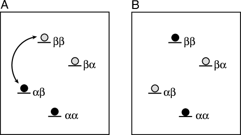
Figure 1: The broadband transfer of polarization $I_{z}$ (A) to $2I_{z}S_{z}$ (B) corresponds to an offset-independent, but transition-selective population inversion of the energy levels $\alpha\beta$ and $\beta\beta$

For large molecules in the so-called spin diffusion limit [17], where longitudinal relaxation rates are negligible compared to transverse relaxation rates, both the initial term ($I_{z}$) and final term ($2I_{z}S_{z}$) of the density operator are long-lived. However, the transfer between these two states requires the creation of coherences which in general are subject to transverse relaxation. The two principal transverse relaxation mechanisms are dipole-dipole (DD) relaxation and relaxation due to chemical shift anisotropy (CSA) of spins $I$ and $S$. The quantum mechanical equation of motion (Liouville-von Neumann equation) for the density operator $\rho$ [17] is given by

$$\dot{\rho} = \pi\ J[-i2I_{z}S_{z},\rho]+\pi\ k_{DD}[2I_{z}S_{z},[2I_{z}S_{z},\rho]]+\pi\ k^{I}_{CSA}[I_{z},[I_{z},\rho]]+\pi\ k^{S}_{CSA}[S_{z},[S_{z},\rho]]$$ (1)

$$+\ \pi\ k^{I}_{DD/CSA}[2I_{z}S_{z},[I_{z},\rho]]+\pi\ k^{S}_{DD/CSA}[2I_{z}S_{z},[S_{z},\rho]],$$

where $J$ is the heteronuclear coupling constant. The rates $k_{DD}$, $k^{I}_{CSA}$, $k^{S}_{CSA}$ represent auto-relaxation rates due to DD relaxation, CSA relaxation of spin $I$ and CSA relaxation of spin $S$, respectively. The rates $k^{I}_{DD/CSA}$ and $k^{S}_{DD/CSA}$ represent cross-correlation rates of spin $I$ and $S$ caused by interference effects between DD and CSA relaxation. These relaxation rates depend on various physical parameters, such as the gyromagnetic ratios of the spins, the internuclear distance, the CSA tensors, the strength of the magnetic field and the correlation time of the molecular tumbling [17]. Let the initial density operator $\rho(0)=A$ and $\rho(t)$ denote the density operator at time $t$. The maximum efficiency of transfer between $A$ and a target operator $C$ is defined as the largest possible value of Trace$\{C^{\dagger}\rho(t)\}$ for any time $t$ [20] (by convention operators A and C are normalized).

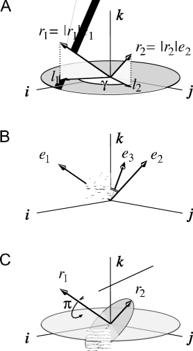
Figure 2: (A) Schematic representation of the magnetization vector $r_{1}=(\langle I_{x}\rangle,\langle I_{y}\rangle,\langle I_{z}\rangle)$ and of the antiphase vector $r_{2}=(\langle 2I_{x}S_{z}\rangle,\langle 2I_{y}S_{z}\rangle,\langle 2I_{z}S_{z}\rangle)$ in the common frame spanned by the standard Cartesian unit vectors ${\bf i}$, ${\bf j}$, and ${\bf k}$. The vectors $l_{1}$ and $l_{2}$ are the projections of $r_{1}$ and $r_{2}$ into the transverse plane and $\gamma$ is the angle between $l_{1}$ and $l_{2}$. (B) For the optimal CROP (cross-correlated relaxation optimized pulse) trajectory [14], the units vectors $e_{1}$, $e_{2}$ in the direction of $r_{1}$ and $r_{2}$ are orthogonal and together with $e_{3}=e_{1}\times e_{2}$ define a specific moving frame along the optimal trajectory. (C) The pulse element $R_{1}(t)$ consists of a $\pi$ rotation of spin $I$ around $e_{1}$, which leaves $r_{1}$ invariant and inverts $r_{2}$ (dashed arrow) and a $\pi$ rotation of spin $S$ around an arbitrary axis in the transverse plane, which also leaves $r_{1}$ invariant and brings $r_{2}$ back to its initial position (solid arrow). Hence, $R_{1}$ neither changes the ratio $|l_{2}|/|l_{1}|$ nor the angle $\gamma$ which are both constants of motion for the optimal CROP trajectory.

In our recent work [14] we showed that for a single spin pair $IS$, the maximum efficiency $\eta$ of transfer between the operators $I_{z}$ and $2I_{z}S_{z}$ depends only on the scalar coupling constant $J$ and the net auto-correlated and cross-correlated relaxation rates of spin $I$, given by $k_{a}=k_{DD}+k^{I}_{CSA}$ and $k_{c}=k^{I}_{DD/CSA}$, respectively. Here the rates $k_{a}$ and $k_{c}$ are a factor of $\pi$ smaller than in conventional definitions of the rates, e.g., $k_{a}=1/(\pi T_{2}$), where $T_{2}$ is the transverse relaxation time in the absence of cross-correlation effects [14, 15]. The physical limit $\eta$ of the transfer efficiency is given by [14]

$$\eta=\sqrt{1+\zeta^{2}}-\zeta,$$ (2)

where $\zeta^{2}={({k_{a}^{2}-k_{c}^{2}})/({J^{2}+k_{c}^{2}})}.$ The optimal transfer scheme (CROP: cross-correlated relaxation optimized pulse) has two constants of motion (see Figure 2 A). If $l_{1}(t)$ and $l_{2}(t)$ denote the two-dimensional vectors $(\langle I_{x}\rangle(t),\langle I_{y}\rangle(t))$ and $(\langle 2I_{x}S_{z}\rangle(t),\langle 2I_{y}S_{z}\rangle(t))$, respectively, then throughout the optimal transfer process the ratio $|l_{2}|/|l_{1}|$ of the magnitudes of the vectors $l_{2}$ and $l_{1}$ should be maintained constant at $\eta$. Furthermore, the angle $\gamma$ between $l_{1}$ and $l_{2}$ is constant throughout. These two constants of motion depend on the transverse relaxation rates and the coupling constants and can be explicitly computed [14]. These constants determine the amplitude and phase of the rf field at each point in time and explicit expressions for the optimal pulse sequence can be derived. In Fig. 3 A and B, the optimal rf amplitude and phase of a CROP sequence is shown as a function of time for the case $k_{c}/k_{a}=0.75$ and $k_{a}=J$.

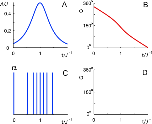
Figure 3: Ideal (A, B) and approximate (C, D) implementations of an on-resonance CROP sequence [14] for $k_{a}=J$ and $k_{c}/k_{a}=0.75$. Panel A shows the ideal rf amplitude $A(t)=-\gamma_{I}B^{I}_{1}(t)/(2\pi)$ (where $\gamma_{I}$ is the gyromagnetic ratio of spins $I$) in units of the coupling constant $J$ and panel C shows a schematic representation of an approximate CROP sequence consisting of 8 hard pulses of flip angle $\alpha=21.5^{\circ}$. Panels B and D show the phases $\varphi(t)$ of the ideal CROP sequence and its hard pulse approximation.

The transfer scheme as described assumes that the resonance frequencies of a single spin pair are known exactly. Therefore, the above methods cannot be directly used in spectroscopic applications with many spin pairs and a dispersion of Larmor frequencies. In this paper, we develop methods to make the above principle of relaxation optimized transfer applicable for a broad frequency range, making these methods suitable for spectroscopy of large proteins. A straightforward method of converting the smooth pulse shapes (like Fig. 3A) into a broadband transfer scheme can be realized by the following steps.

a) Given the optimal amplitude $A(t)$ and phase $\varphi(t)$, of the on-resonance pulse (see Fig. 3 A and 3 B), we can approximate the smooth pulse shape as a sequence of hard pulses with small flip angles $\alpha_{k}$ separated by evolution periods of duration $\Delta_{k}$ (c.f. Figs. 3 C). These are DANTE-type sequences (delays alternating with nutations for tailored excitation) [21]. The flip angle $\alpha_{k}$ at time $t$ is just $\int_{t}^{t+\Delta_{k}}A(\tau)d\tau,$ with the phase given by $\varphi_{k}=\varphi(t)$ (c.f. Fig. 3 D). The delays $\Delta_{k}$ could be chosen in many ways. For example, they may be all equal or can be chosen so that the flip angles $\alpha_{k}$ are equal (c.f. Figs. 3 C).

b) Insertion of $\pi$ pulses in the center of delays to refocus the transverse components of the spins [22], see Fig. 4 A-C.

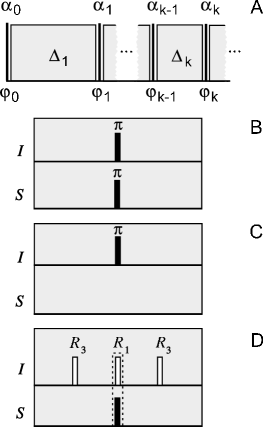
Figure 4: (A) Architecture of broadband relaxation-optimized pulse sequences, consisting of $N$ periods of duration $\Delta_{k}$ (gray boxes, shown in panes B-D in more detail) and hard rf pulses with flip angles $\alpha_{k}$ and phases $\varphi_{k}$. (B) Chemical shift refocusing scheme preserving transfer through $J$ coupling but eliminating transfer though the cross-correlated relaxation rate $k_{c}$. (C) Chemical shift refocusing scheme preserving transfer through $k_{c}$ but eliminating transfer though $J$. (D) STAR echo scheme preserving both transfer through $k_{c}$ and though $J$. In B, C, and D, black bars represent 180^∘ rotations around an axis in the x-y plane, white bars represent 180^∘ rotations around tilted axes.

Note that this method of making relaxation optimized pulses broadband is only applicable if one is using either just the couplings (as in INEPT [18] or ROPE [15] transfer) or just the cross-correlation effects (as in standard CRIPT [19] or CROP [14] transfer for $J=0$) as the transfer mechanism.

For example, the relaxation-optimized pulse elements (ROPE) [15], which only use transfer through couplings (special case of CROP [14] when $k_{c}=0$) can be made broadband in a straight-forward way as explained above. Simultaneous $\pi$ rotations applied to spins $I$ and $S$ in the middle of the evolution periods refocus the chemical shift evolution while retaining the coupling terms (see Fig. 4 B). Note however, that such a pair of $\pi$ rotations will eliminate any DD-CSA cross-correlation effects that might be present [7].

On the other hand, if $J$ is very small or $k_{c}$ is close to $k_{a}$ (in which case transfer using cross-correlation effects is very efficient, c.f. Eq. 2), it is desirable to use relaxation-optimized sequences which only use cross-correlation effects for transfer (special case of CROP [14] when $J=0$). Such a relaxation optimized transfer is characterized by a smooth rotation $I_{z}\rightarrow I_{x}$ and vice versa ($-2I_{x}S_{z}\rightarrow 2I_{z}S_{z}$). Again such a transfer can be made broadband as explained above. In this case the refocusing $\pi$ pulses are applied only to spin $I$ in the center of delays (see Fig. 4 C). By such pulses, cross-correlation effects are retained but coupling evolution is eliminated [7].

Therefore the advantage of the CROP pulse sequence (which simultaneously uses both $J$ couplings and cross-correlation effects) would be lost in using this conventional strategy to make these sequences broadband. The key observation for making CROP transfer broadband is that in the on-resonance CROP transfer scheme, the magnetization vector

$$r_{1}(t)=\langle I_{x}\rangle(t)\ {\bf i}+\langle I_{y}\rangle(t)\ {\bf j}+\langle I_{z}\rangle(t)\ {\bf k}$$

always remains perpendicular (c.f. Fig. 2 A and B) to the net antiphase vector

$$r_{2}(t)=\langle 2I_{x}S_{z}\rangle(t)\ {\bf i}+\langle 2I_{y}S_{z}\rangle(t)\ {\bf j}+\langle 2I_{z}S_{z}\rangle(t)\ {\bf k},$$

where ${\bf i}$, ${\bf j}$, and ${\bf k}$ are the standard Cartesian unit vectors (for details see Supporting Methods). Let $e_{1}$, $e_{2}$ denote unit vectors in the direction of $r_{1}$ and $r_{2}$ and let $e_{3}=e_{1}\times e_{2}$ denote the unit normal pointing out of the plane spanned by $e_{1}$ and $e_{2}$.

Let $R_{1}(t)$ denote a $\pi$ rotation of spin $I$ around $e_{1}(t)$ and a simultaneous $\pi$ rotation of spin $S$ around an arbitrary axis in the transverse plane. Observe that $R_{1}(t)$ fixes the vectors $r_{1}(t)$ and $r_{2}(t)$, see Fig. 2 C. Similarly, let $R_{2}(t)$ denote a $\pi$ rotation around $e_{2}(t)$ and a simultaneous $\pi$ rotation of spin $S$ around an arbitrary axis in the transverse plane. $R_{2}(t)$ inverts $r_{1}(t)$ and $r_{2}(t)$, i.e. $r_{1}(t)\rightarrow-r_{1}(t)$ and $r_{2}(t)\rightarrow-r_{2}(t)$. We also define $R_{3}(t)$ as a $\pi$ rotation around $e_{3}(t)$ which also results in $r_{1}(t)\rightarrow-r_{1}(t)$ and $r_{2}(t)\rightarrow-r_{2}(t)$. Note that these rotations are special because they neither change the ratio $|l_{2}|/|l_{1}|$ nor the angle $\gamma$ between the transverse components $l_{1}$ and $l_{2}$.

We now show how the rotations $R_{1}$ and $R_{3}$ can be used to produce a broadband cross-correlated relaxation optimized pulse (BB-CROP) sequence. Given the implementation of the on resonance CROP pulse (Fig. 3 A and 3 B) as a sequence of pulses and delays (Fig. 3 C and 3 D), the chemical shift evolution during a delay $\Delta$ can be refocused by the sequence (c.f. Fig. 4 D)

$${\Delta\over 4}R_{3}{\Delta\over 4}R_{1}{\Delta\over 4}R_{3}{\Delta\over 4}.$$

The rotations $R_{1}(t)$ and $R_{3}(t)$ are defined using the optimal trajectory and keep changing from one delay to another, as the vectors $r_{1}(t)$ and $r_{2}(t)$ evolve. We refer to this specific trajectory adapted refocusing as STAR. To analyze how this refocusing works, at time instant $t$ consider the coordinate system defined by $e_{1}(t)$, $e_{2}(t)$ and $e_{3}(t)$ (c.f. Fig. 2 B). The unit vector along $z$ can be written as $ae_{1}(t)+be_{2}(t)+ce_{3}(t)$. The chemical shift evolution generator $I_{z}$ can be expressed as

$$I_{z}=aI_{e_{1}}+bI_{e_{2}}+cI_{e_{3}}$$ (3)

and the evolution for time ${{\Delta\over 4}}$ under the chemical shift takes the form $\exp\{-{\rm i}\ \omega(aI_{e_{1}}+bI_{e_{2}}+cI_{e_{3}}){\Delta\over 4}\}$. Assuming that the $R_{3}$ rotation is fast, so that there is negligible chemical shift evolution (and negligible relaxation) during the $R_{3}$, the sequence ${\Delta\over 4}\ R_{3}\ {\Delta\over 4}$ produces the net evolution

$$\exp\{-{\rm i}\ \omega(aI_{e_{1}}+bI_{e_{2}}+cI_{e_{3}}){\Delta\over 4}\}\ \ R_{3}\ \exp\{-{\rm i}\ \omega(aI_{e_{1}}+bI_{e_{2}}+cI_{e_{3}}){{\Delta}\over{4}}\}\ \hskip 20.00003pt$$

$$\ \hskip 20.00003pt=R_{3}\exp\{-{\rm i}\ \omega(-aI_{e_{1}}-bI_{e_{2}}+cI_{e_{3}}){\Delta\over 4}\}\ \exp\{-{\rm i}\ \omega(aI_{e_{1}}+bI_{e_{2}}+cI_{e_{3}}){\Delta\over 4}\}.$$

For delays $\Delta\ll 1/\omega$, the effective evolution can be approximated by $R_{3}\exp\{-{\rm i}\ \omega\ c\ I_{e_{3}}{\Delta\over 2}\}$. Now the rotation $R_{1}$ can be used to refocus the remaining chemical shift evolution due to $I_{e_{3}}$ by the complete STAR echo sequence ${\Delta\over 4}R_{3}{\Delta\over 4}R_{1}{\Delta\over 4}R_{3}{\Delta\over 4}$. The effective evolution during the period $\Delta$

$$R_{1}\exp\{{\rm i}\ \omega cI_{e_{3}}{\Delta\over 2}\}\exp\{-{\rm i}\ \omega cI_{e_{3}}{\Delta\over 2}\}\approx R_{1},$$

i.e. chemical shift evolution is eliminated. Note, we assume that the frame $e_{1}$, $e_{2}$, $e_{3}$ does not evolve much during the four ${\Delta\over 4}$ periods so that the two $R_{3}$ rotations are approximately the same. Under this STAR sequence, the general coupling evolution exp$\{-i2\pi JI_{z}S_{z}\}$ and the general Liouvillian evolution (containing cross correlation effects) is not completely preserved. Inspite of this, the evolution of $r_{1}(t)$ and $r_{2}(t)$ for the CROP trajectory is unaltered. This is because, for this specific trajectory, the magnitude of the transverse components $l_{1}(t)$ and $l_{2}(t)$ and the angle $\gamma$ between them is not changed by application of these tailored refocusing pulses. Since all evolution is confined to transverse operators, the efficiency of the BB-CROP pulse is unaltered by application of STAR refocusing pulses.

3 Practical considerations

180^∘ rotations around tilted axes as required by the operations ($R_{1}$ and $R_{3}$) of the STAR echo method can be realized in practice by off-resonance pulses. For example, a 180^∘ rotation around an axis forming an angle $\theta$ with the $x$ axis can be implemented by a pulse with an rf amplitude $\nu_{1}$ and offset $\nu_{\rm off}=\nu_{1}\tan\theta$ with a pulse duration $\tau_{p}=1/(2\nu_{\rm eff})$, where $\nu^{2}_{\rm eff}=\nu_{1}^{2}+\nu^{2}_{\rm off}$. At the start of the pulse, we assume that both the on-resonance and off-resonance rotating frames are aligned. In the off-resonance rotating frame the axis of rotation does not move. After the pulse, the off-resonant rotating frame has acquired an angle of $\phi_{\rm off}=2\pi\nu_{\rm off}\tau$ relative to the on-resonance frame. For a pulse sequence specified in the on-resonance rotating frame, this can be taken into account by adding the phase $\phi_{\rm off}$ acquired during a given off-resonant 180^∘ pulse to the nominal phases of all following pulses on the same rf channel (In the sequence provided in supporting methods, this correction has been incorporated). Alternative implementations of rotations around tilted axes by composite on-resonance pulses would be longer and could result in larger relaxation losses during the pulses.

Under the assumption of ideal impulsive 180^∘ rotations (with negligible pulse duration and negligible rf inhomogeneity), the STAR approach realizes a broadband transfer of polarization that achieves the optimal efficiency as given in [14]. However, spectrometers are limited in terms of their maximum rf amplitude and homogeneity of the rf field. Therefore in practice, pulses have finite widths and hence evolution (especially relaxation) becomes important during the pulse duration. The effect becomes pronounced as the number of 180^∘ pulses is increased in order to keep the refocusing periods $\Delta_{k}$ short for a better approximation to the on-resonance CROP pulse. We observe that after a point the loss caused due to relaxation during pulse periods overshadows the gain in efficiency one would expect by finer and finer approximations of the ideal CROP trajectory. Furthermore, dephasing due to rf inhomogeneity increases as the number of 180^∘ pulses is increased. Therefore one is forced to find a compromise between loss due to a large number of 180^∘ pulses versus: (a) loss of efficiency due to a coarser discretization of the CROP pulse, (b) reduced bandwidth of frequencies that can be refocused by an increased duration of the refocusing periods. When the number of refocusing periods becomes small, it is important to find a good way to discretize the CROP pulse so as to maximize the efficiency of coherence transfer that can be achieved by a pulse sequence with a prescribed number of evolution periods. We have developed rigorous control theoretic methods based on the principle of dynamic programming [26] to efficiently achieve this discretization (see Supporting Methods). This helps us to compute optimal approximations of CROP pulse sequences as a series of a small number of pulses and delays very efficiently.

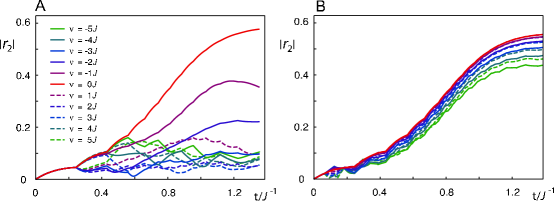
Figure 5: The buildup of antiphase vectors $r_{2}$ is shown for 11 different offset frequencies in the range of $\pm 5J$ during (A) a selective CROP (without STAR echoes) and (B) a corresponding BB-CROP (with STAR echoes) sequence consisting of 12 periods $\Delta_{k}$. The sequence was optimized for $k_{a}=J$ and $k_{c}/k_{a}=0.75$ and a maximum rf amplitude of $67\ J$.

Fig. 5 A shows the buildup of antiphase vectors $r_{2}$ for 11 different offset frequencies in the range of $\pm 5J$ (corresponding to $\pm 1$ kHz for $J\approx 200$ Hz) during a CROP sequence consisting of 12 periods $\Delta_{k}$ without STAR echoes. As expected, the optimal transfer efficiency is only achieved for spins close to resonance. In contrast, a corresponding BB-CROP experiment with STAR refocusing produces efficient polarization transfer for a large range of offsets (c.f. Fig. 5B). Figure 6 shows how the BB-CROP sequence ”locks” the angle $\gamma$ between $l_{2}$ and $l_{1}$ (c.f. Fig. 2) near its optimal value as given by on-resonance CROP pulse.

We have carried out extensive simulations to study the loss in efficiency due to a large number of 180^∘ pulses for realistic as well as hypothetical values of rf amplitudes. Fig. 7 illustrates how the offset dependence of the transfer efficiency $\eta$ is effected by increasing the number of STAR echo periods both in the absence and presence of rf inhomogeneity. From the figures it is clear that one has to find an optimal number of evolution periods that gives the best performance for given system parameters like maximum rf amplitude, rf inhomogeneity and the bandwidth one desires to cover.

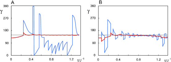
Figure 6: Evolution of the angle $\gamma$ during the selective CROP (A) and BB-CROP (B) sequence as in Fig. 5 for the on-resonance case (red curves) and for an offset of -3 $J$. The optimal value of $\gamma$ to be maintained during the CROP trajectory is indicated by dashed lines.

It is important to note that with high-resolution spectrometers, equipped with more rf power, relaxation losses during pulse periods can be made very small. This is illustrated in Figs. 7 A and B, assuming a maximum rf amplitude on the $I$ channel of $500\ J$ and 67$J$, respectively, corresponding to 180^∘ pulse durations of 5 $\mu$s and 39 $\mu$s (typical value for ¹³C pulses) for the $J\approx 194$ Hz coupling constant of the ¹³C-¹H spin pair of a model system [14, 15], (vide infra). For short 180^∘ pulses (large rf amplitude) during which relaxation losses become small, a larger number of refocusing pulses has the largest bandwidth and approaches the ideal CROP efficiency most closely (c.f. green curve in Fig. 7 A).

The refocusing sequence ${\Delta\over 4}R_{3}{\Delta\over 4}R_{1}{\Delta\over 4}R_{3}{\Delta\over 4}$ as described in the theory section is not the only STAR refocusing scheme for making CROP sequences broadband. For example, ${\Delta\over 4}R_{3}{\Delta\over 4}R_{2}{\Delta\over 4}R_{3}{\Delta\over 4}$ or ${\Delta\over 4}R_{2}{\Delta\over 4}R_{1}{\Delta\over 4}R_{2}{\Delta\over 4}$ will also perform STAR refocusing. However as indicated above, in practice it may be necessary to have $\Delta$ as large as possible, in which case one should try to refocus the largest of the components $a$, $b$, $c$ of the chemical shift generator $I_{z}$ (c.f. Eq. 3) more often during the refocusing cycle $\Delta$. For example, the choice of the refocusing cycle presented in the paper is optimal for the values of $k_{c}/k_{a}=0.75$ and $k_{a}/J=1$, in which case the vector $e_{3}$ is mostly in the x-y plane and hence the magnitude of component $c$ is smaller than the magnitude of $a$ or $b$. Therefore it is of advantage to refocus $a$ and $b$ more often by performing $R_{3}$ rotations (the $R_{3}$ rotation refocuses the $a$ and $b$ components) and hence the choice of the sequence. Since there are no rotations of spin $S$ during the application of $R_{3}$ pulses, the total number of pulses and the resulting effects due to rf inhomogeneity are minimized. Dephasing losses due to rf inhomogeneity of the 180^∘ pulses (e.g. applied to spin $S$) can be further reduced by choosing appropriate phase cycling schemes [23, 24, 25].

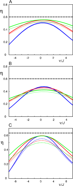
Figure 7: Offset dependence of the transfer efficiency $\eta$ for system parameters corresponding to the ¹³C-¹H moiety of ¹³C sodium formate in glycerol with $k_{a}=J$ and $k_{c}/k_{a}=0.75$ [14] (A, B) and corresponding to the ¹H-¹⁵N moiety of a protein with a a rotational correlation time of 70 ns with $k_{a}=0.8\ J$ and $k_{c}/k_{a}=0.73$ [7] (A and B). A maximum rf amplitude on the $I$ channel of 500 $J$ (A), $67\ J$ (B), and 550 $J$ (C) is assumed, corresponding to a hypothetical 180^∘ (¹³C) pulse duration of 5 $\mu$s (A), realistic on-resonance 180^∘ (¹³C) pulse duration of 39 $\mu$s (B) and a 180^∘(¹H) pulse duration of 10 $\mu$s (C) for a ¹H-¹⁵N coupling of $J=93$ Hz. Blue, red and green curves represent BB-CROP sequences with 4, 8 and 12 STAR echo periods $\Delta_{k}$, respectively (for details, see Supporting Methods). Solid and dashed curves correspond to simulations in the absence and presence of rf inhomogeneity, respectively, assuming a Gaussian rf distribution with a full width at half height of 10%.

In many cases it might also be possible to cut down relaxation losses by suitable implementation of the 180^∘ pulses. For example, in the presence of a large contribution of the dipole-dipole mechanism to the transverse relaxation rates, synchronization of $I$ and $S$ rotations can be used to create transverse bilinear operators such as $I_{x}S_{x}$ which commute with $I_{z}S_{z}$. This way some of the losses might be prevented when the antiphase magnetization is passed through the transverse plane during its inversion by $R_{3}$ pulses.

4 Experimental results

In order to test the BB-CROP pulse sequence, we chose an established model system [14, 15], consisting of a small molecule (¹³C-labeled sodium formate) dissolved in a highly viscous solvent ((²H₈) glycerol) in order to simulate the rotational correlation time of a large protein. Both the simplicity and sensitivity of the model system makes it possible to quantitatively compare the transfer efficiency of pulse sequences and to acquire detailed offset profiles in a reasonable time. Because of its large chemical shift anisotropy and the resulting CSA-DD cross-correlation effects, we use the ¹³C spin of ¹³C-sodium formate to represent spin $I$ and the attached ¹H spin to represent spin $S$ with a heteronuclear scalar coupling constant of $J=193.6$ Hz. At a temperature of 270.6 K and a magnetic field of 17.6 T, the experimentally determined auto and cross-correlated relaxation rates of spin $I$ were $k_{a}\approx J$ and $k_{c}\approx 0.75\ k_{a}$ (solvent: 100% (²H₈) glycerol). For a given pulse sequence element, the achieved transfer efficiency of ¹³C polarization $I_{z}$ to $2I_{z}S_{z}$ was measured by applying a hard 90${}_{y}^{\circ}$ proton pulse and recording the resulting proton anti-phase signal (initial ¹H magnetization was dephased by applying a 90^∘ proton pulse followed by a pulsed magnetic field gradient) [15].

Figure 8: Experimental on-resonance transfer efficiencies of the CROP (open square) and corresponding BB-CROP (filled square) sequence consisting of four periods $\Delta_{k}$ (without and with STAR echoes) and a total duration of 4.2 ms. For comparison, experimental on-resonance INEPT and CRIPT transfer efficiencies are shown as a function of the transfer time. In the experiments, spins $I$ and $S$ correspond to ¹³C and ¹H in ¹³C-sodium formate dissolved in (²H₈) glycerol.

Fig. 8 shows experimental on-resonance transfer efficiencies of the conventional INEPT [18] and CRIPT [19] sequences as a function of the mixing time. The figure also shows the on-resonance transfer efficiency of a CROP sequence consisting of four periods $\Delta_{k}$ (without refocusing) which shows a gain of 65% compared to the maximum INEPT efficiency. As expected (c.f. blue curve in Fig. 7 B), the broadband version of this sequence (BB-CROP) with four STAR echoes has a reduced transfer efficiency because of relaxation losses during the additional 180^∘ pulses, which in the current experiments had relatively long durations due to the relatively small rf amplitude (13 kHz) of the $I$ channel (¹³C) (the BB-CROP pulse sequence is provided in Supporting Methods). Additional losses are caused by dephasing due to rf inhomogeneity, which is typically larger for the ¹³C channel (where most 180^∘ pulses are given) compared to the ¹H channel. The experimentally determined on-resonance transfer efficiency of BB-CROP is 28 % larger than the maximum INEPT transfer efficiency. In Fig. 9, the experimental offset profiles of the $I_{z}\rightarrow 2I_{z}S_{z}$ transfer efficiency of BB-CROP and INEPT are compared. A reasonable match is found between the experiments and the simulations shown in Fig. 7 B.

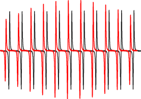
Figure 9: Experimental offset dependence of the $I_{z}\rightarrow 2I_{z}S_{z}$ transfer efficiency for a BB-CROP sequence consisting of 4 periods with STAR echoes (red) and the INEPT sequence (black). The resulting two-spin order $2I_{z}S_{z}$ was converted to antiphase coherence $2I_{z}S_{x}$ by a hard $90^{\circ}(S)$ pulse and the resulting antiphase signals are shown for 11 offsets of spin $I$ in the range of $\pm$ 500 Hz.

5 Conclusion

In this paper we introduced the principle of specific trajectory adapted refocusing (STAR), which was used to design broadband relaxation optimized BB-CROP pulse sequence. We would like to emphasize again that with increasing rf amplitudes, the efficiency of the on-resonance cross-correlated relaxation optimized pulse can be closely approached by the BB-CROP sequences. As future spectrometers are equipped with more rf power, we can significantly reduce the duration of 180^∘ refocusing pulses, which are the major bottleneck in BB-CROP achieving the maximum efficiency. Based on our simulations, we expect immediate gains in NMR spectroscopy of large proteins by use of the proposed BB-CROP pulses. For example, in the HSQC experiment involving ¹H and ¹⁵N, with maximum rf amplitudes corresponding to 12 $\mu$s ¹H 180^∘ pulses and 40 $\mu$s ¹⁵N 180^∘ pulses, we expect up to 70% enhancement in sensitivity over a reasonable bandwidth compared to state of the art methods. With currently available rf amplitudes, in many applications it might even be advantageous to use broadband versions of ROPE or optimal CRIPT (special case of CROP where $J=0$). In these cases, we only use 180^∘ pulses in the center of each evolution period and hence loose less due to relaxation during the pulses (of course, as pointed out earlier, in these cases in order to do a broadband transfer, we will necessarily eliminate either J couplings or cross-correlation ). In Figs. 8 and 9 we have not compared the sensitivity of BB-CROP with CRINEPT [7] as the latter is not broadband for the transfer $I_{z}\rightarrow 2I_{z}S_{z}$. Similar to the on-resonance CROP pulse, we have found that the BB-CROP pulse sequence is robust to variations in relaxation rates. Finally, the ability of the BB-CROP sequence to achieve the maximum possible transfer efficiency over a broad frequency range by use of high rf power provides a strong motivation to build high-resolution spectrometers with short 180^∘ pulses.

6 Supporting Methods

6.1 Orthogonality of inphase and antiphase magnetization along CROP trajectories

Let $r_{1}(t),r_{2}(t)$ represent the inphase and antiphase magnetization vectors as defined in the paper. Let $l_{1}$ and $l_{2}$ represent their transverse components as shown in Fig. 1 of the main text. For the sake of simplicity of notation, we will also use $l_{1}$ and $l_{2}$ to denote the magnitudes of these transverse vectors, as the true meaning will be clear from the context. In [14], it was shown that the CROP transfer $I_{z}\rightarrow 2I_{z}S_{z}$ has the following properties. Throughout the transfer, the angle $\gamma$ between vectors $l_{1}$ and $l_{2}$ is constant and the ratio $\frac{l_{2}}{l_{1}}$ is constant at the value $\eta$, where $\eta$ is the optimal efficiency of the CROP pulse. The two constants of motion completely determine the amplitude $A$ and the phase $\phi$, the CROP pulse makes with the vector $l_{1}$. Furthermore $\gamma$ and $\eta$ satisfy [14]

$$\frac{1}{\eta}\cos(\theta-\gamma)+\eta\cos(\theta+\gamma)=\frac{2\xi}{\chi},$$ (4)

where $\xi=\frac{k_{a}}{J}$, $\chi=\sqrt{1+\frac{k_{c}^{2}}{J^{2}}}$ and $\theta=\tan^{-1}(\frac{J}{-k_{c}})$.

Using $z_{1}(t)=\langle I_{z}\rangle(t)$ and $z_{2}(t)=\langle 2I_{z}S_{z}\rangle(t)$, the inner product $J$ between $r_{1}(t)$ and $r_{2}(t)$ can be expressed as

$$J=z_{1}(t)z_{2}(t)+l_{1}(t)l_{2}(t)\cos(\gamma).$$

We now compute $\frac{dJ}{dt}$ along the CROP trajectory using the following identities, where the time dependence of the quantities, $l_{1},l_{2},z_{1},z_{2},A,\phi$ is implicit.

$$\frac{dz_{1}}{dt} = -2\pi Al_{1}\sin\phi$$

$$\frac{dz_{2}}{dt} = 2\pi A\ l_{2}\sin(\gamma-\phi)$$

$$\frac{dl_{1}}{dt} = 2\pi A\ z_{1}\sin\phi-\pi J(\xi\ l_{1}-\chi\ l_{2}\cos(\theta+\gamma))$$

$$\frac{dl_{2}}{dt} = -2\pi A\sin(\gamma-\phi)\ z_{2}-\pi J(\xi\ l_{2}-\chi\ l_{1}\cos(\theta-\gamma))$$

$$\frac{dJ}{dt}=l_{1}l_{2}\{A\sin\gamma(\frac{z_{1}}{l_{1}}\cos\phi-\frac{z_{2}}{l_{2}}\cos(\gamma-\phi))+J\chi\ (\frac{l_{1}}{l_{2}}\cos(\theta-\gamma)+\frac{l_{2}}{l_{1}}\cos(\theta+\gamma)-2\frac{\xi}{\chi})\}.$$

Along the CROP trajectory, $\frac{d\gamma}{dt}=0$ implies [14]

$$A\sin\gamma\ (\frac{z_{1}}{l_{1}}\cos\phi-\frac{z_{2}}{l_{2}}\cos(\gamma-\phi))=0.$$

Also along the CROP trajectory $\frac{l_{2}}{l_{1}}=\eta$. Using (Eq. 4), we then obtain that along CROP trajectory

$$\frac{l_{1}}{l_{2}}\cos(\theta-\gamma)+\frac{l_{2}}{l_{1}}\cos(\theta+\gamma)=\frac{2\xi}{\chi}.$$

This then implies $\frac{dJ(t)}{dt}=0$. Since $J(0)=0$ as $r_{2}(0)=0$, we obtain that throughout the transfer $J(t)=0$.

6.2 Dynamic Programming method for finding optimal sequence of flips and delays

We now explain the method of dynamic programming [26] for finding the optimal sequence of pulses and delays that best approximates relaxation optimized pulse sequences. The method is best illustrated by considering the simpler case when there is no cross-correlation in the system. In absence of cross-correlation, the relaxation optimized transfer of $I_{z}\rightarrow 2I_{z}S_{z}$ is characterized by gradual rotation of the operator $I_{z}\rightarrow I_{x}$, followed by the rotation $2I_{y}S_{z}\rightarrow 2I_{z}S_{z}$ [15]. Let $r_{1}$ be the magnitude of in-phase terms, i.e., $r_{1}^{2}=\langle I_{x}\rangle^{2}+\langle I_{z}\rangle^{2}$. Let $\beta_{1}$ be the angle $r_{1}$ makes with the transverse plane, i.e. $\beta_{1}=\cos^{-1}{{\langle I_{x}\rangle}\over{r_{1}}}$ (see Fig. 1). Let $r_{2}$ measure the magnitude of the total antiphase terms, i.e., $r_{2}^{2}=\langle 2I_{y}S_{z}\rangle^{2}+\langle 2I_{z}S_{z}\rangle^{2}$ and let $\beta_{2}=\cos^{-1}{{\langle 2I_{y}S_{z}\rangle}\over{r_{2}}}$ (see Fig. 1). Using rf fields, we can exactly control the angle $\beta_{1}$ and $\beta_{2}$ and these are thought of as control parameters (see Fig. 1). During the evolution of relaxation optimized pulse sequence [15] one of the $\beta_{1}$ or $\beta_{2}$ is zero, so we assume $(\beta_{1},\beta_{2})\in([0,\frac{\pi}{2}],0)\cup(0,[0,\frac{\pi}{2}])$.

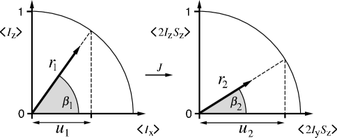
Figure 10: Representation of the system variables $r_{1}$, $r_{2}$, the angles $\beta_{1}$, $\beta_{2}$, and of the control parameters $u_{1}=\cos\beta_{1}$, $u_{2}=\cos\beta_{2}$ in terms of the expectation values $\langle I_{x}\rangle$, $\langle I_{z}\rangle$, $\langle 2I_{y}S_{z}\rangle$, and $\langle 2I_{z}S_{z}\rangle$.

Now suppose, we only have one evolution period, consisting of a pulse and delay, at our disposal. We can compute this optimal pulse and delay so that at the end of the evolution period, $r_{2}$ is maximized. Starting with $r_{1},r_{2}$ as defined and a given choice of $\beta_{1}$, $\beta_{2}$ and $\tau$, the values of $r_{1}(\tau)$ and $r_{2}(\tau)$ at the end of the period $\tau$ are

$$r_{1}^{2}(\tau) = \exp(-2\pi k_{a}\tau)(r_{1}\cos\beta_{1}\cos(\pi J\tau)-r_{2}\cos\beta_{2}\sin(\pi J\tau))^{2}+(r_{1}\sin\beta_{1})^{2}$$ (5)

$$r_{2}^{2}(\tau) = \exp(-2\pi k_{a}\tau)(r_{2}\cos\beta_{2}\cos(\pi J\tau)+r_{1}\cos\beta_{1}\sin(\pi J\tau))^{2}+(r_{2}\sin\beta_{2})^{2}.$$ (6)

We write this as $(r_{1}(\tau),r_{2}(\tau))=f(r_{1},r_{2};\beta_{1},\beta_{2},\tau)$. We can maximize the expression in equation (6) and find the optimal value of $\tau,\beta_{1},\beta_{2}$ and also the largest achievable value $r_{2}(\tau)$. This value depends only on the initial value $r_{1}$ and $r_{2}$ and we call it $V_{1}(r_{1},r_{2})$, the optimal return function at stage 1 starting from $r_{1},r_{2}$. This optimal return function represents the best we can do starting from a given value of $r_{1}$ and $r_{2}$ given only one evolution period.

Given two evolution periods, then by definition $V_{2}(r_{1},r_{2})=\max_{\beta_{1},\beta_{2},\tau}V_{1}(f(r_{1},r_{2};\beta_{1},\beta_{2},\tau))$. The basic idea is, since we have computed $V_{1}$ for various values of $r_{1}$ and $r_{2}$ , we can use it to compute $V_{2}$. In general then

$$V_{n}(r_{1},r_{2})=\max_{\beta_{1},\beta_{2},\tau}V_{n-1}(f(r_{1},r_{2};\beta_{1},\beta_{2},\tau)).$$ (7)

Thus the dynamic programming proceeds backwards. We first compute the optimal return functions $V_{1}$ followed by $V_{2}$ and so on. Computing $V_{k}(r_{1},r_{2})$, also involves computing the best value of the control parameters $\beta_{1},\beta_{2},\tau$ to choose for a given value of state $r_{1},r_{2}$ at stage $k$. We denote this optimal choice as $\beta_{1}^{\ast}(r_{1},r_{2},k),\beta_{2}^{\ast}(r_{1},r_{2},k),\tau^{\ast}(r_{1},r_{2},k)$, indicating that the optimal control depends on the state $r_{1},r_{2}$ and the stage $k$.

In practice, the algorithm is implemented by sampling the $[0,1]\times[0,1]$ square in the $r_{1},r_{2}$ plane uniformly into say 100 points. Each of these points correspond to a different value of $r_{1},r_{2}$. By maximizing the expression in equation 6, we can compute the optimal $\beta_{1},\beta_{2},\tau$ for each of these points. This would give us $\beta_{1}^{\ast}(r_{1},r_{2},1),\beta_{2}^{\ast}(r_{1},r_{2},1),\tau^{\ast}(r_{1},r_{2},1)$ and also $V_{1}(r_{1},r_{2})$. Now to find $V_{2}(r_{1},r_{2})$ at these points, we sample the control space $(\beta_{1},\beta_{2})\in([0,\frac{\pi}{2}],0)\cup(0,[0,\frac{\pi}{2}])$ and $\tau\in[0,\frac{1}{2J}]$ uniformly and compute the value $f(r_{1},r_{2},\beta_{1},\beta_{2},\tau)$ for all of these samples $\beta_{1},\beta_{2},\tau$ and choose the one that has the largest value $V_{1}(f(r_{1},r_{2};\beta_{1},\beta_{2},\tau))$ .This then is the best choice of control parameters if there are two evolution periods to go. We also then obtain $V_{2}(r_{1},r_{2})=V_{1}(f(r_{1},r_{2},\beta_{1}^{\ast},\beta_{2}^{\ast},\tau^{\ast}))$. We can continue this way and compute $V_{n}(r_{1},r_{2})$. Now to construct the optimal pulse sequence consisting of $N$ evolution periods, we just look at the value $\beta_{1}^{\ast}(1,0,N),\beta_{2}^{\ast}(1,0,N),\tau^{\ast}(1,0,N)$ and evolve the system according to these parameters and get $r_{1}$ and $r_{2}$ at beginning of stage $N-1$. But we also know $\beta_{1}^{\ast}(r_{1},r_{2},N-1),\beta_{2}^{\ast}(r_{1},r_{2},N-1),\tau^{\ast}(r_{1},r_{2},N-1)$ which is then used to evolve the system for one more step and so on. From the sequence $\beta_{1}^{\ast}(r_{1},r_{2},k),\beta_{2}^{\ast}(r_{1},r_{2},k),\tau^{\ast}(r_{1},r_{2},k)$,  $k=1...N$, the optimal flip angles can be immediately determined.

6.3 BB-CROP Pulse sequence parameters

Table 1: Parameters of a BB-CROP sequence (c.f. Fig. 4 A and D) consisting of four STAR echoes optimized for $k_{a}/J=1$, $k_{c}/k_{a}=0.75$ and amplitude $A=67\ J\approx 13$ kHz of the $I$ channel for $J=193.6$ Hz. The DANTE-type on-resonance pulses applied to spin $I$ are denoted $\alpha_{k}$. The Table only specifies explicitly the parameters for the spin $I$ rf channel, however note that the pulse elements $R_{1}(t)$ require a simultaneous hard 180^∘ rotation of spin $S$ around an axis in the transverse plane. In our experiments, the phases of the four 180${}^{\circ}(S)$ pulses were chosen according to the XY-4 cycle 0^∘, 90^∘, 0^∘, 90^∘ [24] in order to reduce the effects of rf inhomogeneity of the $S$ pulses.

type	duration [$\mu$s]	offset [kHz]	Phase [deg]
$\alpha_{0}$	5.9	-	0
$\Delta_{1}/4$	300.2	-	-
$R_{3}(t)$	36.1	$-4.77$	119.5
$\Delta_{1}/4$	300.2	-	-
$R_{1}(t)$	12.7	$37.13$	20.9
$\Delta_{1}/4$	300.2	-	-
$R_{3}(t)$	37.6	$-2.76$	224.6
$\Delta_{1}/4$	300.2	-	-
$\alpha_{1}$	7.9	-	393.9
$\Delta_{2}/4$	220.2	-	-
$R_{3}(t)$	34.1	-6.82	182.5
$\Delta_{2}/4$	220.2	-	-
$R_{1}(t)$	25.1	15.13	36.3
$\Delta_{2}/4$	220.2	-	-
$R_{3}(t)$	35.5	-5.39	223.5
$\Delta_{2}/4$	220.2	-	-
$\alpha_{2}$	8.6	-	340.5
$\Delta_{3}/4$	219.7	-	-
$R_{3}(t)$	34.5	-6.42	157.3
$\Delta_{3}/4$	219.7	-	-
$R_{1}(t)$	35.2	5.74	353.8
$\Delta_{3}/4$	219.7	-	-
$R_{3}(t)$	34.4	-6.48	136.6
$\Delta_{3}/4$	219.7	-	-
$\alpha_{3}$	7.9	-	217.3
$\Delta_{4}/4$	301.2	-	-
$R_{3}(t)$	36.7	-4.04	58.3
$\Delta_{4}/4$	301.2	-	-
$R_{1}(t)$	38.3	-1.19	269.0
$\Delta_{4}/4$	301.2	-	-
$R_{3}(t)$	36.4	-4.49	344.1
$\Delta_{4}/4$	301.2	-	-
$\alpha_{4}$	4.2	-	350.3

References

- [1] Redfield, A. G. (1957) IBM J. Res. Dev. 1, 19-31.
- [2] Wüthrich, K. (1986) NMR of Proteins and Nucleic Acids, (Wiley, New York)
- [3] Cavanagh, J., Fairbrother W. J., Palmer A. G. & Skelton, N. J. (1996) Protein NMR Spectroscopy, Principles and Practice, (Academic Press, New York).
- [4] Pervushin, K., Riek, R., Wider, G. & Wüthrich, K. (1997) Proc. Natl. Acad. Sci. USA 94, 12366-12371.
- [5] Salzmann, M., Pervushin, K., Wider, G., Senn, H. & Wüthrich, K. (1998) Proc. Natl. Acad. Sci. USA 95, 13585-13590.
- [6] Wüthrich, K. (1998) Nat. Struct. Biol. 5, 492-495.
- [7] Riek, R., Wider, G., Pervushin, K. & Wüthrich, K. (1999) Proc. Natl. Acad. Sci. USA 96, 4918-4923.
- [8] McConnell, H. M. (1956) J. Chem. Phys. 25, 709-711.
- [9] Shimizu, H. (1964) J. Chem. Phys. 40, 3357-3364.
- [10] Ayscough, P. B. (1967) Electron Spin Resonance in Chemistry (Methuen, London).
- [11] Vold, R. R. & Vold, R. L. (1978) Prog. NMR Spectrosc. 12, 79-133.
- [12] Goldman, M. (1984) J. Magn. Reson. 60, 437-452.
- [13] Kumar, A., Grace, R. C. & Madhu, P. K. (2000) Prog. NMR Spectrosc. 37, 191-319.
- [14] Khaneja, N. Luy, B. & Glaser, S. J. (2003) Proc. Natl. Acad. Sci. USA 100, 13162-13166.
- [15] Khaneja, N., Reiss, T., Luy, B. & Glaser, S. J. (2003) J. Magn. Reson. 162, 311-319.
- [16] Stefanatos, D., Khaneja, N. & Glaser, S. J. (2004) Phys. Rev. A 69, 022319.
- [17] Ernst, R. R., Bodenhausen, G. & Wokaun, A. (1987) Principles of Nuclear Magnetic Resonance in One and Two Dimensions, (Clarendon Press, Oxford).
- [18] Morris, G. A. & Freeman, R. (1979) J. Am. Chem. Soc. 101, 760-762.
- [19] Brüschweiler, R. & Ernst, R. R. (1992) Chem. Phys. 96, 1758-1766.
- [20] Glaser, S. J., Schulte-Herbrüggen, T., Sieveking, M., Schedletzky, O., Nielsen, N. C., Sørensen, O. W. & Griesinger, C. (1998) Science. 208, 421-424.
- [21] Morris, G. A. & Freeman, R. (1978) J. Magn. Reson. 29, 433-462.
- [22] Reiss, T. O., Khaneja, N. & Glaser, S. J. (2003) J. Magn. Reson. 165, 95-101.
- [23] Levitt, M. H. (1982) J. Magn. Reson. 48, 234-264.
- [24] Gullion, T., Baker, D. B. & Conradi, M. S. (1990) J. Magn. Reson. 89, 479-484.
- [25] Tycko R. & Pines, A. (1985) J. Chem. Phys. 83, 2775-2802.
- [26] Bellman, R. (1957) Dynamic Programming (Princeton University Press, Princeton).