Adiabatic pulse propagation in coherent atomic media with the tripod level configuration

Abstract

We investigate the problem of propagation of three-component resonant light pulses with adiabatically varying amplitudes through a medium consisting of atoms with the tripod level configuration. By means of both analytic and numerical methods we found the two modes of shape-preserving pulse propagation. The pulse propagation velocity is found to be either equal to the speed of light or significantly slowed down, depending on a particular propagation mode.

]

I Introduction

Coherent population trapping (CPT) is a well-known phenomenon of preparation of atoms in a coherent superposition of ground or metastable state sublevels (so-called dark state), which is immune to excitation by a two-component laser radiation under the two-photon resonance condition [1]. Since the laser radiation is not scattered by atoms in the dark state, the radiation absorption is dramatically reduced. This effect is called electromagnetically induced transparency (EIT) and is actively studied since early 90’s [2]. One of the most striking features of EIT is possibility of shape-preserving propagation of light pulses with slowly (adiabatically) varying amplitudes at the group velocity significantly reduced with respect to the speed of light in vacuum, $c$ [3]. Shape-preserving electromagnetic pulses propagating in a coherent atomic medium at the reduced group velocity were called in Ref. [3] “adiabatons”. Experimental observations of light a pulse group velocity less by many orders of magnitude than $c$ has been repeatedly reported [4]. Slowing down the laser light followed by spatial compression of the pulses provides a unique possibility for design of nonlinear-optical devices operating on a few-photon level [5]. Extreme sensitivity of CPT and EIT to deviations from the two-photon resonance allowed to observe experimentally large Kerr nonlinearity [6] and absorptive optical switching [7] in cold rubidium vapor. Such nonlinear optical phenomena, along with the possibility of reversible conversion of a photonic excitation to a collective spin excitation [8] and trapping light in a medium with the photonic band gap induced by a periodic modulation of the EIT resonance [9], are of great importance for quantum information storage and processing.

A novel direction in CPT and EIT studies is related to the systems admitting more than one dark state for the given real Rabi frequencies, $|\Omega_{j}|$, and phases, $\chi_{j}$, associated with the resonantly driven transitions. The simplest scheme of such a kind is the tripod scheme displayed in Fig. 1. Stimulated Raman adiabatic passage (STIRAP) in such an optically thin atomic medium with the tripod level scheme was investigated theoretically [10] and demonstrated experimentally [11] by Bergmann and co-workers. A proposal to use the tripod scheme as a physical implementation of a qubit has been made recently [12]. A 5-level scheme being the extension of the tripod scheme was considered in Ref. [13].

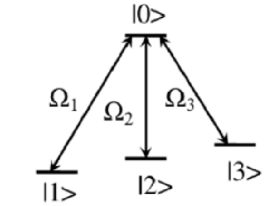
FIG. 1.: Tripod scheme of levels driven by resonant electromagnetic fields.

The very specifics of the tripod scheme is that during adiabatically slow change of the external field parameters transitions between the two dark state occurs. These transitions are described by a non-Abelian phase matrix [14], which is a generalization of a geometric (Berry) phase [15] to the case of degenerate eigenstates of an adiabatic Hamiltonian. One may expect that these transitions give rise to rich and complicated dynamics of laser pulse propagation in an optically dense medium with the tripod level configuration. However, only few theoretical works on EIT in such media are available. Paspalakis and Knight [16] considered parametric frequency generation for the case of time-independent fields at the medium entrance and calculated the group velocity of a weak probe field. Petrosyan and Malakyan [17] investigated theoretically EIT in a tripod medium as a tool for optical cross-phase modulation and high-precision magnetometry in the weak probe field limit. The value of the group velocity obtained in [16, 17] is strongly reduced with respect to $c$ in the same way as in the standard case of EIT in a three-level medium [3]. In the theoretical interpretation of the experiment on four-wave mixing in a solid-state system with the tripod level configuration [18] and other numerical calculations by Ham [19] related to that system, small optical density of the medium was assumed.

The aim of the present paper is to study pulse propagation in a medium with the tripod level scheme (hereafter briefly called “tripod medium”) for a general case, in which none of the three resonant electromagnetic fields is assumed to be weak compared to others. The paper is organized as follows. In Sec. II we present the set of equations treating pulse propagation in the adiabatic regime in a tripod medium beyond the weak probe approximation . In Sec. III the analytic solutions describing slow and fast pulse propagation are obtained. Sec. IV contains the results of our numerical calculations and their interpretation. Sec. V deals with some particular regimes of propagations. Sec. VI is devoted to conclusive remarks.

II Basic equations

If the three electromagnetic fields are tuned exactly in resonance with the corresponding transitions $\left|j\right\rangle\leftrightarrow\left|0\right\rangle$, $j=1,2,3$, the Hamiltonian in the interaction representation reads as

$$\hat{H}=-\hbar\sum_{j=1}^{3}\Omega_{j}\left|0\right\rangle\left\langle j\right|+\mathrm{H.c.},$$ (1)

$\Omega_{j}\equiv|\Omega_{j}|e^{i\chi_{j}}=d_{0j}E_{j}/\hbar$, where $d_{0j}$ is the dipole moment matrix element of the given transition. The electric field in the $j$th laser wave is $E_{j}\exp[ik_{j}(z-t/c)]+\mathrm{c.c.}$, $k_{j}$ being the radiation wave number. The complex amplitude $E_{j}$ is a slowly varying function of $z$ and $t$. Expanding the atomic wave function as $\left|\psi\right\rangle=a_{0}\left|0\right\rangle+\sum_{j=1}^{3}a_{j}\left|j\right\rangle$, we obtain the Schrödinger equation for the probability amplitudes:

$$i\dot{a}_{j} = -\Omega_{j}^{*}a_{0},\quad j=1,2,3,$$ (2)

$$i\dot{a}_{0} = -\sum_{j=1}^{3}\Omega_{j}a_{j}.$$ (3)

The set of shortened Maxwell equations for slowly varying field amplitudes can be written as

$$\left(\frac{\partial}{\partial z}+\frac{1}{c}\frac{\partial}{\partial t}\right)\Omega_{j}=iG_{j}a_{0}a_{j}^{*},\quad j=1,2,3,$$ (4)

where $G_{j}=2\pi k_{j}nd_{0j}^{2}/\hbar$ and $n$ is the atomic number density. Taking into consideration propagation effects described by Eq. (4) is the essence of the theory developed in the present Section, in contrast to the theory of Ref. [10], which applies to the case of a refractively thin medium.

Hereafter we assume that all the matter-field coupling constants are equal:

$$G_{1}=G_{2}=G_{3}\equiv G.$$ (5)

Violation of this assumption leads to adiabaticity breakdown during the pulse propagation and subsequent pulse front steepening [20]. Thermal motion of atoms leads, besides reduction of the effective number density of atoms in resonance with the laser radiation, to a similar effect of pulse front steepening [21]. However, the pulse shape distortion effects manifest themselves at propagation distances much larger than the typical propagation distance associated with an adiabaton-like pulse formation [20, 21]. Therefore we can neglect both the differences of oscillator strengths associated with the three laser-driven transitions and thermal motion of atoms. We also neglect the radiative decay of the excited state $\left|0\right\rangle$ since it plays no role in the adiabatic regime, because of negligible population of the excited state [3].

We parameterize the Rabi frequencies by introducing the generalized Rabi frequency $\Omega=\left(\sum_{j=1}^{3}|\Omega_{j}|^{2}\right)^{1/2}$ and two angular variables $\varphi$ and $\vartheta$:

$$\Omega_{1} = \sin\vartheta\cos\varphi\,e^{i\chi_{1}}\Omega,$$ (6)

$$\Omega_{2} = \cos\vartheta\cos\varphi\,e^{i\chi_{2}}\Omega,$$ (7)

$$\Omega_{3} = \sin\varphi\,e^{i\chi_{3}}\Omega.$$ (8)

There are two mutually orthogonal non-absorbing (dark) states associated with the Hamiltonian of Eq. (1):

$$\left|\Phi^{(1)}\right\rangle = \cos\vartheta\,e^{-i\chi_{1}}\left|1\right\rangle-\sin\vartheta\,e^{-i\chi_{2}}\left|2\right\rangle,$$ (9)

$$\left|\Phi^{(2)}\right\rangle = \sin\vartheta\sin\varphi\,e^{-i\chi_{1}}\left|1\right\rangle+$$ (11)

$$\cos\vartheta\sin\varphi\,e^{-i\chi_{2}}\left|2\right\rangle-\cos\varphi\,e^{-i\chi_{3}}\left|3\right\rangle.$$

An atom initially prepared in either of these two states remains unexcited since

$$\hat{H}\left|\Phi^{(s)}\right\rangle=0,\quad s=1,2.$$ (12)

An atom also remains unexcited if the parameters of the laser radiation vary in time slowly enough to satisfy the adiabaticity conditions

$$\dot{\vartheta}\ll\Omega,~{}\qquad\dot{\varphi}\ll\Omega,$$ (13)

and

$$\dot{\chi}_{j}\ll\Omega,~{}\quad j=1,2,3.$$ (14)

However, in the latter case there are transitions [14] between the dark states defined by Eqs. (11), where the instantaneous values of the varying angles $\varphi$ and $\vartheta$ and phases $\chi_{j}$ enter. If at $t\rightarrow-\infty$ an atom was in the $s$th dark state, its wave function at subsequent instants of time is

$$\left|\Psi^{(s)}\right\rangle=\sum_{s^{\prime}=1}^{2}B_{ss^{\prime}}(t)\left|\Phi^{(s^{\prime})}\right\rangle,$$ (15)

where the matrix $\hat{B}$ obeys the equation

$$\dot{B}_{ss^{\prime}}(t)+\sum_{s^{\prime\prime}}B_{ss^{\prime\prime}}(t)A_{s^{\prime}s^{\prime\prime}}(t)=0$$ (16)

with the initial condition

$$B_{ss^{\prime}}(-\infty)=\delta_{ss^{\prime}},$$ (17)

and

$$A_{s^{\prime}s^{\prime\prime}}(t)=\left\langle\Phi^{(s^{\prime})}\right|\frac{\partial}{\partial t}\left|{\Phi}^{(s^{\prime\prime})}\right\rangle.$$ (18)

Explicitly,

$$A_{11} = -i(\dot{\chi}_{1}\cos^{2}\vartheta+\dot{\chi}_{2}\sin^{2}\vartheta),$$ (19)

$$A_{12} = \dot{\vartheta}\sin\varphi-i(\dot{\chi}_{1}-\dot{\chi}_{2})\sin\vartheta\cos\vartheta\sin\varphi,$$ (20)

$$A_{21} = -A_{12}^{*},$$ (21)

$$A_{22} = -i[(\dot{\chi}_{1}\sin^{2}\vartheta+\dot{\chi}_{2}\cos^{2}\vartheta)\sin^{2}\varphi+$$ (23)

$$\dot{\chi}_{3}\cos^{2}\varphi].$$

It is easy to show that if the phases of the laser fields are kept constant at the medium entrance, then

$$\dot{\chi}_{j}=0,\quad j=1,2,3,$$ (24)

in the whole tripod medium. The opposite is not true. If the absolute values of the field amplitudes are constant at the medium entrance, but the phases are modulated, then the absolute values of the fields amplitudes and, hence, $\vartheta$ and $\varphi$ become time-dependent inside the medium. In the present paper we consider only the case when Eq. (24) holds. In this case Eqs. (23) are reduced to

$$A_{11}=A_{22}=0,\qquad A_{12}=-A_{21}=\dot{\nu},$$ (25)

where

$$\dot{\nu}=\dot{\vartheta}\sin\varphi$$ (26)

and $\nu(z,-\infty)=0$. Then Eqs. (16, 17) yield the following result [10]:

$$B_{11}=B_{22}=\cos\nu,\qquad B_{12}=-B_{21}=\sin\nu.$$ (27)

We assume that the tripod medium occupies the half-space $z>0$. Initially, at $t\rightarrow-\infty$, all the atoms in the medium are in the coherent superposition of the dark states

$$\left|\psi(-\infty)\right\rangle=\cos\beta\left|\Phi^{(1)}\right\rangle+\sin\beta\left|\Phi^{(2)}\right\rangle.$$ (28)

The boundary conditions for the fields at the medium entrance $\Omega(0,t)=\Omega_{0}(t)$, $\vartheta(0,t)=\vartheta_{0}(t)$, and $\varphi(0,t)=\varphi_{0}(t)$ are consistent with Eq. (13). Thus the adiabatic regime of the laser radiation propagation inside the medium is ensured. It is convenient to introduce new variables $\zeta=z$ and $\tau=t-z/c$, as in Ref. [3]. Respectively, the derivatives over the new variables are $\partial/(\partial\tau)=\partial/(\partial t)$ and $\partial/(\partial\zeta)=\partial/(\partial z)+c^{-1}\partial/(\partial t)$.

Now we can solve self-consistently the set of Schrödinger — Maxwell equations (3, 4). First of all, we note that in the adiabatic regime $a_{0}$ is very small, and the probability amplitudes of the low-energy states ($j=1,2,3$) are, according to Eqs. (15, 27, 28),

$$a_{j}=\cos(\nu+\beta)\left\langle j\right|\Phi^{(1)}\left.\right\rangle+\sin(\nu+\beta)\left\langle j\right|\Phi^{(2)}\left.\right\rangle.$$ (29)

Then we find easily, that, similarly to the case of adiabatic pulse propagation in a $\Lambda$-medium [3],

$$\frac{\partial}{\partial\zeta}\Omega=0,$$ (30)

i.e., $\Omega=\Omega_{0}(\tau)$. Then we use the trick first applied in Ref. [3]: We express the small probability amplitude of the excited state as $a_{0}=-(i/\Omega_{j}^{*})\partial a_{j}/(\partial\tau)$ and substitute this expression into the shortened Maxwell equations (4). We get $\partial|\Omega_{j}/\Omega|^{2}/(\partial\zeta)=(G/\Omega^{2})\partial|a_{j}|^{2}/(\partial\tau)$, $j=1,2,3$, or, explicitly,

$$\frac{\partial}{\partial\zeta}(\sin\vartheta\cos\varphi)^{2} = \frac{\partial}{\partial w}[\cos(\nu+\beta)\cos\vartheta+$$ (32)

$$\sin(\nu+\beta)\sin\vartheta\sin\varphi]^{2},$$

$$\frac{\partial}{\partial\zeta}(\cos\vartheta\cos\varphi)^{2} = \frac{\partial}{\partial w}[-\cos(\nu+\beta)\sin\vartheta+$$ (34)

$$\sin(\nu+\beta)\cos\vartheta\sin\varphi]^{2},$$

$$\frac{\partial}{\partial\zeta}\sin^{2}\varphi = \frac{\partial}{\partial w}[\sin(\nu+\beta)\cos\varphi]^{2}.$$ (35)

Here we introduced, instead of $\tau$, a new variable (nonlinear time)

$$w=\frac{1}{G}\int_{-\infty}^{\tau}\Omega_{0}^{2}(\tau^{\prime})\,d\tau^{\prime},$$ (36)

which has the dimension of length. Then Eq. (26) takes the form

$$\frac{\partial\nu}{\partial w}=\frac{\partial\vartheta}{\partial w}\sin\varphi.$$ (37)

All the initial conditions set at $t\rightarrow-\infty$ apply now to $w=0$.

Only two of Eqs. (35) are independent. After some tedious calculations they are reduced to

$$\frac{\sin(\nu+\beta)}{\cos\varphi}\left(\frac{\partial}{\partial\zeta}+\frac{\partial}{\partial w}\right)\varphi-$$ (38)

$$\cos(\nu+\beta)\left(\frac{\partial}{\partial\zeta}+\frac{\partial}{\partial w}\right)\vartheta = 0,$$ (39)

$$\frac{\cos(\nu+\beta)}{\cos\varphi}\frac{\partial\varphi}{\partial\zeta}+\sin(\nu+\beta)\frac{\partial\vartheta}{\partial\zeta} = 0.$$ (40)

It is convenient now to change the variables to $u_{1}=\zeta-w$ and $u_{2}=w$. The set of Eqs. (37, 40) takes the form

$$\frac{\cos(\nu+\beta)}{\cos\varphi}\frac{\partial\varphi}{\partial u_{1}} + \sin(\nu+\beta)\frac{\partial\vartheta}{\partial u_{1}}=0,$$ (41)

$$\frac{\sin(\nu+\beta)}{\cos\varphi}\frac{\partial\varphi}{\partial u_{2}} - \cos(\nu+\beta)\frac{\partial\vartheta}{\partial u_{2}}=0,$$ (42)

$$\frac{\partial\nu}{\partial u_{1}}-\frac{\partial\nu}{\partial u_{2}} = \left(\frac{\partial\vartheta}{\partial u_{1}}-\frac{\partial\vartheta}{\partial u_{2}}\right)\sin\varphi.$$ (43)

III Slow and fast pulses: The analytic solution

The set of Eqs. (41 – 43) is especially convenient for searching analytic solutions in a case when the unknown functions $\varphi$ and $\vartheta$ depend on only one of the variables $u_{1},~{}u_{2}$. We find two classes of solutions.

The first one is the class of slow pulses. In this case the unknown functions depend only on $u_{1}=\zeta-w$. The group velocity $v_{g}$ of pulses of such has the same form as that of adiabatons in a $\Lambda$-medium [3]: $v_{g}=\left(c^{-1}+G/\Omega^{2}\right)^{-1}$ and can be much less than $c$. All the derivatives over $u_{2}$ vanish, thus making Eq. (42) an identity. The two remaining equations (41) and (43) become ordinary differential equations, yielding the general solution in the parametric form:

$$|\cos\varphi|=\frac{C_{1}}{|\cos(\nu+\beta)|},\quad|\sin(\vartheta-C_{2})|=\frac{|\sin(\nu+\beta)|}{\sqrt{1-C_{1}^{2}}}.$$ (44)

Here $C_{1},~{}C_{2}$ are arbitrary constants, and $p$ is any function of $\zeta-w$ compatible with the adiabaticity conditions (13).

Similarly, we find a general solution for the class of fast pulses, propagating at the speed of light:

$$|\cos\varphi|=\frac{C_{3}}{|\sin(\nu+\beta)|},\quad|\sin(\vartheta-C_{4})|=\frac{|\cos(\nu+\beta)|}{\sqrt{1-C_{3}^{2}}}.$$ (45)

Here $C_{3},~{}C_{4}$ are arbitrary constants, and $p=p(w)$ must be compatible with Eq. (13).

Although the set of Eqs. (41 – 43) looks rather simple and symmetric, our attempts to find its general solution in the case of dependence of $\varphi$ and $\vartheta$ on both $u_{1}$ and $u_{2}$ have been unsuccessful. However, we can prove that a time-dependent solution in the parametric form

$$\varphi=\varphi(p),\qquad\vartheta=\vartheta(p)$$ (46)

does not exist if

$$\frac{\partial p}{\partial u_{1}}\neq 0,\qquad\frac{\partial p}{\partial u_{2}}\neq 0.$$ (47)

Indeed, Eqs. (41, 42) can be considered as linear homogeneous algebraic equations for $\sin(\nu+\beta)$ and $\cos(\nu+\beta)$. They have a solution if

$$\frac{\partial\vartheta}{\partial u_{1}}\frac{\partial\vartheta}{\partial u_{2}}+\frac{1}{\cos^{2}\varphi}\frac{\partial\varphi}{\partial u_{1}}\frac{\partial\varphi}{\partial u_{2}}=0.$$ (48)

But if we make an assumption given by Eq. (46) then Eq. (48) results in

$$\frac{\partial p}{\partial u_{1}}\frac{\partial p}{\partial u_{2}}\left[\left(\frac{d\vartheta}{dp}\right)^{2}+\frac{1}{\cos^{2}\varphi}\left(\frac{d\varphi}{dp}\right)^{2}\right]=0.$$ (49)

If Eq. (47) holds, it follows from Eq. (49) that $\varphi=\mathrm{const}$ and $\vartheta=\mathrm{const}$, i.e., there is no variation of the electromagnetic fields in space and time.

The fact that we have not found other pulse group velocities than $c$ and $\left(c^{-1}+G/\Omega^{2}\right)^{-1}$ is in full agreement with the results of perturbative approach [16, 17].

IV Numerical solutions

It is natural to expect that any pulse of finite duration evolves in the medium into pair of fast and slow pulses, which become more and more separated in space due to the difference of their group velocities. Indeed, our numerical simulations confirm such an expectation. An example is shown in Fig. 2. The quantity $w_{0}$ used for normalization of the horizontal axes of the plots in Fig. 2 and subsequent determines the order of magnitude of $\dot{\varphi}$ and $\dot{\vartheta}$, which are $\sim\Omega^{2}/(Gw_{0})$. The adiabaticity condition (13) results in the following restriction: $w_{0}\gg\Omega/G$. One can see that the incident pulse evolves into a well separated pair of fast (F) and slow (S) pulses, and the mixing angle $\nu$ describing transitions between the two dark states emerges (the incident pulse is chosen in such a form that $\nu\equiv 0$ at the medium entrance). The F and S pulses at large propagation distances can be excellently fitted with formulae (45) and (44), respectively.

We also investigated numerically collisions between fast and slow pulses. The results are presented in Fig. 3. The pulse sequence is organized in such a way that the pulse of a shape satisfying Eq. (44) enters the medium first. After some time delay the next pulse obeying Eq. (45) enters the medium. The first pulses propagates at the slow group velocity whereas the second one propagates at the speed of light. The distance between them decreases, and at certain $\zeta$ the two pulses overlap (this is marked by O in Fig. 3b). Their nonlinear interaction leads to strong distortion of their shapes, which becomes apparent at larger propagation distances. Thus adiabatic pulses in a tripod medium cannot be called solitons in the exact sense of soliton definition by Zabusky and Kruskal [22]. Note that it is impossible to arrange a collision of two adiabatons in a $\Lambda$-medium.

The parameter $\beta$ is equal to 1.12 for Fig. 2 and 1.87 for Fig. 3.

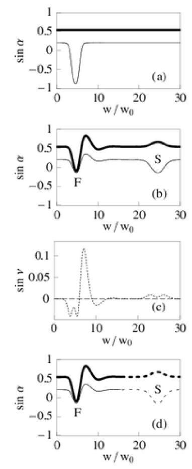
FIG. 2.: Splitting of the incident pulse into the fast (F) and slow (S) pulses. (a) Sine functions of the angles $\alpha=\vartheta$ (thick line) and $\varphi$ (thin line) versus scaled nonlinear time, $w/w_{0}$, at the medium entrance, $\zeta=0$ (the boundary conditions); the same line styles are reserved for $\vartheta$ and $\varphi$ in all the subsequent figures. (b) The same as in (a) for $\zeta=20w_{0}$ (numerical simulation results). (c) Sine of mixing angle $\nu$ versus $w/w_{0}$ for $\zeta=0$ (dashed line) and $20w_{0}$ (dotted line). (d) Fitting of the plot (b) with Eq. (45) (solid lines; $C_{1}=0.88$, $C_{2}=1.75$) and Eq. (44) (dashed lines; $C_{3}=0.43$, $C_{4}=-0.90$. Axes are in dimensionless units in all plots.

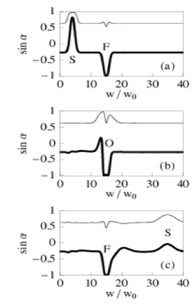
FIG. 3.: Collision of pulses. (a) Sine functions of the angles $\alpha=\vartheta$ and $\varphi$ versus $w/w_{0}$ at $\zeta=0$ (the boundary conditions). (b) The same as in (a) for $\zeta=10w_{0}$ (numerical simulation results). (c) The same as in (b) for $\zeta=30w_{0}$. See the text for more detailed description.

V Particular regimes of propagation

There are a few particular regimes of adiabatic pulse propagation admitting analytic treatment. The first one occurs if atoms are prepared initially in a statistical mixture described by the density matrix $\hat{\varrho}=\frac{1}{2}\left(\left|\Phi^{(1)}\right\rangle\left\langle\Phi^{(1)}\right|+\left|\Phi^{(2)}\right\rangle\left\langle\Phi^{(2)}\right|\right)$, rather than in a pure state. Such a mixed state remains invariant under the action of action of the slowly varying electromagnetic fields: $\hat{B}\hat{\varrho}\hat{B}^{\dagger}=\hat{\varrho}$, where $\hat{B}$ is given by Eq. (27). Statistical averaging over $\hat{\varrho}$ is equivalent to averaging over the parameter $\beta$ uniformly distributed between 0 and $2\pi$, without any correlation with the instantaneous values of $\varphi$ and $\vartheta$. The result of statistical averaging of Eqs. (35) is

$$\frac{\partial\varphi}{\partial\zeta}=-\frac{1}{2}\frac{\partial\varphi}{\partial w},\qquad\frac{\partial\vartheta}{\partial\zeta}=-\frac{1}{2}\frac{\partial\vartheta}{\partial w}.$$ (50)

Equations for $\varphi$ and $\vartheta$ become decoupled. Their solution $\varphi=\varphi_{0}(w-\frac{1}{2}\zeta)$, $\vartheta=\vartheta_{0}(w-\frac{1}{2}\zeta)$ describes independent propagation of perturbations of $\vartheta$ and $\varphi$ at the same group velocity $v_{g}=\left[c^{-1}+G/(2\Omega^{2})\right]^{-1}$.

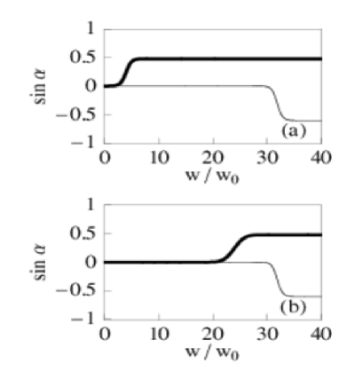
FIG. 4.: Adiabatic pulse propagation for the particular initial condition $\beta=0$. (a) Sine functions of the angles $\alpha=\vartheta$ and $\varphi$ versus $w/w_{0}$ at $\zeta=0$ (the boundary conditions). (b) The same as in (a) for $\zeta=20w_{0}$ (numerical simulation results).

We may hazard a conjecture what occurs if atoms are prepared in a mixed state with the density matrix $\hat{\varrho}^{\prime}=q\left|\Phi^{(1)}\right\rangle\left\langle\Phi^{(1)}\right|+(1-q)\left|\Phi^{(2)}\right\rangle\left\langle\Phi^{(2)}\right|$, $0\leq q\leq 1$. It is likely that there are always two classes of pulses with well defined group velocities. If $q$ grows from 0 to 0.5, one of these velocities decreases whereas the other increases. At $q=0.5$ they achieve the same value mentioned in the previous paragraph, and then again restore their values $c$ and $(c^{-1}+G/\Omega^{2})^{-1}$, as $q$ approaches 1. At least, it can be proven easily in the perturbative regime, when the changes of both $\varphi$ and $\vartheta$ are small.

Another interesting regime is related to particular initial conditions $\beta=0$ or $\beta=\pi/2$. Let all the atoms be pumped initially into the state $\left|3\right\rangle$. The fields are switched on in the following order, which is a generalization of the counterintuitive pulse order for a $\Lambda$-medium [3]: Initially, at $w=0$ only the field driving the empty transition $\left|2\right\rangle\leftrightarrow\left|0\right\rangle$ is present, i.e., $\varphi=\vartheta=0$. Obviously, $\beta=0$. Then the field driving the transition $\left|1\right\rangle\leftrightarrow\left|0\right\rangle$ is switched on adiabatically, so that $\vartheta$ grows and then is kept constant at a certain level. Finally, the field driving the transition $\left|3\right\rangle\leftrightarrow\left|0\right\rangle$ is switched on.

When $\vartheta$ changes, $\sin\varphi=0$. Then, according to Eq. (26), $\nu$ remains zero, and Eqs. (40) are reduced to $\partial\varphi/(\partial u_{1})=0$, $\partial\vartheta/(\partial u_{2})=0$. Such a propagation regime occurs unless the front of the $\vartheta$-pulse, propagating at the slow group velocity, approaches the front of the $\varphi$-pulse, propagating at $c$.

Thus one has a possibility of preparation of a tripod medium in any desired coherent superposition of low-energy states. Numerical results presented in Fig. 3 illustrate this conclusion: Finally, atoms in the region $0<z<20w_{0}$ are prepared in the state $-0.29\left|1\right\rangle-0.53\left|2\right\rangle-0.80\left|3\right\rangle$, as can be derived from the values $\varphi=-0.65$, $\vartheta=0.50$ at $w=40w_{0}$. Then one can suddenly change the laser radiation parameters in such a manner that this state will correspond to a coherent superposition of the two dark states defined with respect to the new values of the Rabi frequencies, thus obtaining a new value for the parameter $\beta$.

The case of $\beta=\pi/2$ is physically equivalent to the previous one, differing only in notation of the states and electromagnetic fields.

VI Conclusion

Requirements for experimental implementation of adiabatic pulse propagation in a tripod medium should not differ from that for slow light propagation in $\Lambda$-media [2, 4, 8]. A method for initial preparation of a tripod medium in any desired superposition state was outlined in the previous section. For example, consider a tripod medium with the following parameters: $d_{0j}\approx 10^{-18}$ esu$\,\cdot\,$cm, $k_{j}\approx 10^{5}$ cm^-1, $n\approx 10^{12}$ cm^-3. Let the total laser intensity be of about 3 mW/cm² (slightly below the atomic transition saturation limit). Hence, $\Omega\approx 2.4\cdot 10^{6}$ s^-1 and $\Omega^{2}/G\approx 10^{4}$ cm/s (i.e., the group velocity of the slow pulses is $v_{g}\approx 0.3\cdot 10^{-6}c$). The value of the scaling parameter of the horizontal axes of the Figs. 2 – 4 $w_{0}\approx 0.1$ cm is thus large enough to provide adiabaticity. Therefore the processes illustrated in Fig. 2–4 can be observed in a few centimeter long gas cell. The time delay between the fast and slow pulses is of about 0.3 ms, therefore the lifetime of coherence between the states $\left|j\right\rangle$, $j=1,2,3$, should be 1 ms or longer. It is achievable in coated cells or cells with a buffer gas.

To conclude, we have investigated electromagnetic pulse propagation in a coherent atomic medium with the tripod configuration of levels in the adiabatic regime. The propagation equations (41 – 43) are derived and their solutions in the form of slow [Eq. (44)] and fast [Eq. (45)] pulses are obtained analytically. Our numerical simulations confirm that these solutions are general asymptotic solutions for any incident pulse of a finite duration. We have suggested a method of preparation of a tripod medium in an arbitrary superposition of the low-energy states based on switching on the laser fields in a counterintuitive order. The tripod scheme provides two novel features in comparison to the $\Lambda$-scheme. The first one is adiabatic pulse propagation in a medium prepared in a statistical mixture of the two dark states. The second one is the possibility of collisions between the slow and fast pulses revealing that they change their shapes after nonlinear interaction and thus do not satisfy the classical definition of a soliton [22].

The author thanks L. Windholz, E.V. Galaktionov, and D.G. Yakovlev for useful discussions. The work is supported by the Austrian Science Foundation (project P 14645) and the program Leading Russian Scientific Schools (grant 1115.2003.2).

REFERENCES

- [1] E. Arimondo, in: E. Wolf (Ed.), Progress in Optics, vol. 35, North-Holland, Amsterdam, 1996, p.259.
- [2] S.E. Harris, Phys. Today 50, No. 7, 36 (1997).
- [3] R. Grobe, F.T. Hioe, J.H. Eberly, Phys. Rev. Lett. 73 , 3183 (1994).
- [4] A. Kasapi, M. Jain, G. Y. Yin, S. E. Harris, Phys. Rev. Lett. 74, 2447 (1995); O. Schmidt, R. Wynands, Z. Hussein, D. Meschede, Phys. Rev. A 53, R27 (1996); L.V. Hau, S.E. Harris, Z. Dutton, C.H. Behroozi, Nature 397, 594 (1999); M.M. Kash, V.A. Sautenkov, A.S. Zibrov, L. Hollberg, G.R. Welch, M.D. Lukin, Yu. Rostovtsev, E.S. Fry, M.O. Scully, Phys. Rev. Lett. 82, 5229 (1999); D. Budker, D.F. Kimball, S.M. Rochester, V.V. Yashchuk, Phys. Rev. Lett. 83, 1767 (1999); E. Podivilov, B. Sturman, A. Shumelyuk, S. Odoulov, Phys. Rev. Lett. 91, 083902 (2003).
- [5] S.E. Harris, L.V. Hau, Phys. Rev. Lett. 82, 4611 (1999).
- [6] H. Kang, Y. Zhu, Phys. Rev. Lett. 91, 093601 (2003).
- [7] D.A. Braje, V. Balić, G.Y. Yin, S.E. Harris, Phys. Rev. A 68, 041801 (2003).
- [8] M.D. Lukin, Pev. Mod. Phys. 75, 457 (2003).
- [9] A. André, M.D. Lukin, Phys. Rev. Lett. 89, 143602 (2002); M. Bajcsy, A.S. Zibrov, M.D. Lukin, Nature, 426, 638 (2003).
- [10] R. Unanyan, M. Fleischhauer, B.W. Shore, K. Bergmann, Opt. Commun. 155, 144 (1998); R. Unanyan, B.W. Shore, K. Bergmann, Phys. Rev. A 59, 2910 (1999).
- [11] H. Theuer, R.G. Unanyan, C. Habscheid, K. Klein, K. Bergmann, Opt. Express 4, 77 (1999).
- [12] Z. Kis, F. Renzoni, Phys. Rev. A 65, 032318 (2002).
- [13] Z. Kis, S. Stenholm, Phys. Rev. A 64, 063406 (2001).
- [14] F. Wilczek, A. Zee, Phys. Rev. Lett. 52, 2111 (1984).
- [15] M.V. Berry, Proc. R. Soc. London, Ser. A 392, 45 (1984).
- [16] E. Paspalakis, P.L. Knight, J. Opt. B: Quant. Semiclass. Opt. 4, S372 (2002).
- [17] D. Petrosyan, Yu.P. Malakyan, e-print: quant-ph/0402070.
- [18] B.S. Ham, P.R. Hemmer, Phys. Rev. Lett. 84, 4080 (2000).
- [19] B.S. Ham, Appl. Phys. Lett. 78, 3382 (2001).
- [20] I.E. Mazets and B.G. Matisov, Quant. Semiclass. Opt. 8, 909 (1996).
- [21] I.E. Mazets, Phys. Rev. A 54, 3539 (1996).
- [22] N.J. Zabusky and M.D. Kruskal, Phys. Rev. 15, 240 (1965).