Ghost Interference with Optical Parametric Amplifier

Abstract

The ’Ghost’ interference experiment is analyzed when the source of entangled photons is a multimode Optical parametric Amplifier(OPA) whose weak limit is the two-photon Spontaneous Parametric Downconversion(SPDC) beam. The visibility of the double-slit pattern is calculated, taking the finite coincidence time window of the photon counting detectors into account. It is found that the coincidence window and the bandwidth of light reaching the detectors play a crucial role in the loss of visibility on coincidence detection, not only in the ’Ghost’ interference experiment but in all experiments involving coincidence detection. The differences between the loss of visibility with two-mode and multimode OPA sources is also discussed.

I Introduction

The ’Ghost’ interference experiment is typical of two-photon interference experiments that bring out quantum entanglement features of light. These features are not just confined to the appearance of the double-slit pattern on coincidence detection. The independence of the result on where the optical elements are situated in the experimental set-up (a double-slit in the case of ’Ghost’ interference) is a key feature of entanglement. The ’Ghost’ interference experiment has been performed in the low-gain limit of parametric down-conversion shih . It is of interest to examine this experiment in the high gain regime of parametric amplification. Analysis of similar experiments using two-mode OPA states boyd suggest the loss of visibility at large gains. Recently different detection schemes have been proposed to circumvent this problem  gatti1 ; gatti2 . Here we present a detailed calculation of the ’Ghost’ interference experiment using a multimode OPA as the source of entangled photons. We analyze the effect of the coincidence time window of the photon counting detectors on the experimentally observable interference pattern and visibility. We attempt to explain how the properties of the source of entangled photons and experimental limitations affect the observable interferometric effects. We find that the loss of visibility depends on the coincidence time window and the bandwidth of the source. The coincidence time window causes a loss in visibility at much lower gains than expected with ideal detectors. A multimode source causes loss in visibility even if ideal detectors are used. Combined with a finite coincidence time window, a multimode source can reduce visibility to less than 0.5 even at very low parametric gain. These effects are not specific to the ’Ghost’ interference experiment but occur in all experiments with similar sources and detection schemes.

II Multimode interaction in OPA

We consider a non-degenerate OPA mollow comprising a non-centrosymmetric crystal with a second order non-linear susceptibility $\chi^{(2)}$. The crystal is pumped by a CW laser, given by

$$E_{p}(\vec{r},t) = E_{p}^{(+)}+E_{p}^{(-)}$$ (1)

$$= E_{p}e^{i(\vec{k}_{p}\cdot\vec{r}-\omega_{p}t)}+H.c$$ (2)

where H.c stands for Hermitian conjugate. We assume that the pump is not depleted, has a constant amplitude $E_{p}$ and can be treated classically. If a weak multimode signal is also input into the OPA, the output after parametric interaction within the crystal consists of amplified modes of the signal and idler where the idler modes obey the phase matching conditions,

$$\omega_{p} = \omega_{s}+\omega_{i}$$ (3)

$$\vec{k}_{p} = \vec{k}_{s}+\vec{k}_{i}$$ (4)

where $\vec{k}_{p}$, $\vec{k}_{s}$ and $\vec{k}_{i}$ are the wave vectors of the pump, signal and idler photons. The quantized field of the signal and idler inside the crystal are given by  glauber ,

$$E_{s}(\vec{r},t) = \sum_{k_{s}}\sqrt{\frac{\hbar\omega_{s}}{2\epsilon_{0}V}}e^{i(\vec{k}_{s}\cdot\vec{r}-\omega_{s}t)}a_{\vec{k}_{s}}+H.c$$ (5)

$$E_{i}(\vec{r},t) = \sum_{k_{s}}\sqrt{\frac{\hbar\omega_{i}}{2\epsilon_{0}V}}e^{i(\vec{k}_{i}\cdot\vec{r}-\omega_{i}t)}a_{\vec{k}_{i}}+H.c$$ (6)

Here $a_{\vec{k}}$ is the annihilation operator for a photon in mode $\vec{k}$. Note that the dispersion relation $\omega(k)$ is different from that in vacuum, $\omega(k)\neq ck$.

The non-linear interaction between the crystal, the pump, signal and idler modes are characterized by the interaction Hamiltonian klyshko  louisell ,

$$H_{int} = 2\epsilon_{0}\chi^{(2)}\int d^{3}rE_{p}^{(+)}E_{s}^{(-)}E_{i}^{(-)}+H.c$$ (7)

$$= 2\epsilon_{0}\chi^{(2)}\sum_{k_{s},k_{i}}\sqrt{\frac{\hbar\omega_{s}}{2\epsilon_{0}V}}\sqrt{\frac{\hbar\omega_{i}}{2\epsilon_{0}V}}E_{p}\times$$

$$\int d^{3}r[e^{i(\vec{k}_{p}-\vec{k}_{s}-\vec{k}_{i})\cdot\vec{r}}e^{i(\omega_{s}+\omega_{i}-\omega_{p})t}a^{\dagger}_{\vec{k}_{s}}a^{\dagger}_{\vec{k}_{i}}$$

$$+e^{-i(\vec{k}_{p}-\vec{k}_{s}-\vec{k}_{i})\cdot\vec{r}}e^{-i(\omega_{s}+\omega_{i}-\omega_{p})t}a_{\vec{k}_{s}}a_{\vec{k}_{i}}]$$

where the integration is over the volume of the crystal illuminated by the pump. For a long crystal and a wide pump beam,

$$\int d^{3}re^{i(\vec{k}_{p}-\vec{k}_{s}-\vec{k}_{i})\cdot\vec{r}}=V\delta_{\vec{k}_{p}-\vec{k}_{s},\vec{k}_{i}}$$ (8)

The interaction Hamiltonian is simplified to

$$H_{int} = 2\epsilon_{0}\chi^{(2)}V\sum_{k_{s},k_{i}}\sqrt{\frac{\hbar\omega_{s}}{2\epsilon_{0}V}}\sqrt{\frac{\hbar\omega_{i}}{2\epsilon_{0}V}}E_{p}\delta_{\vec{k}_{p}-\vec{k}_{s},\vec{k}_{i}}$$

$$\left[e^{i(\omega_{s}+\omega_{i}-\omega_{p})t}a^{\dagger}_{\vec{k}_{s}}a^{\dagger}_{\vec{k}_{i}}+e^{-i(\omega_{s}+\omega_{i}-\omega_{p})t}a_{\vec{k}_{s}}a_{\vec{k}_{i}}\right]$$

The delta function in Eq. (II) indicates the entanglement of the OPA states in wave vector space. Combining the photon commutation relations and the time evolution equations for signal and idler modes, the time-evolved signal and idler are given by scully ; walls ,

$$a_{\vec{k}_{s}}(t) = a_{\vec{k}_{s}}(0)cosh(|\xi_{k_{s}}|)-ia^{\dagger}_{\vec{k}_{i}}(0)sinh(|\xi_{k_{s}}|)$$ (10)

$$a^{\dagger}_{\vec{k}_{i}}(t) = a^{\dagger}_{\vec{k}_{i}}(0)cosh(|\xi_{k_{s}}|)+ia_{\vec{k}_{s}}(0)sinh(|\xi_{k_{s}}|)$$ (11)

where $t$ is the average time taken by the photons to cross the crystal. $a_{\vec{k}_{s}}(0)$ and $a^{\dagger}_{\vec{k}_{i}}(0)$ are the annihilation and creation operators for the input signal and idler mode. The factors $cosh(|\xi_{k_{s}}|)$ and $sinh(|\xi_{k_{s}}|)$ are the amplification factors that depend on the strength of the non-linearity $\chi^{(2)}$,the pump $E_{p}$ and the frequency of the signal and idler modes. Perfect phase-matching ensures that each signal mode interacts with only one idler mode, selected by the phase-matching conditions. Eq’s. (10) and (11) relate the photon creation annihilation operators at the output face of the crystal to those at the input. They are derived from the unitary transformation,

$$U_{k_{i}}=e^{\left[\frac{\xi_{k_{s}}^{\ast}}{2}a_{\vec{k}_{s}}(0)a_{\vec{k}_{i}}(0)-\frac{\xi_{k_{s}}}{2}a^{\dagger}_{\vec{k}_{s}}(0)a^{\dagger}_{\vec{k}_{i}}(0)\right]}$$ (12)

Here $\xi_{k_{s}}=(\chi^{(2)}E_{p}\sqrt{\omega_{s}\omega_{i}}t)e^{i\pi/2}$, may be recognized as the squeeze parameter of the OPA scully . The state at the output of the crystal is given by

$$|\psi\rangle=e^{-i\left(\frac{H_{int}}{\hbar}t\right)}|0\rangle$$ (13)

which is a multiphoton state. In the limit $|\xi_{k_{s}}|\ll 1$, the expansion of Eq. (13) can be limited to first order in the interaction Hamiltonian, giving a vacuum state and an entangled two-photon state. This is the two-photon limit of SPDC.

III Experimental Set-up and Calculation

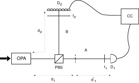
Figure 1: Schematic of the experimental setup for observing the two-photon ’Ghost’ interference. For simplicity, the prism to remove the pump is not shown. The double-slit has width $b=0.165$ mm and slit distance $a=0.4$ mm. The relevant distances in this experiment are $d_{1}=0.3$ m, $d_{2}=1.5$ m, and $d^{{}^{\prime}}_{1}=1$ m.

We now look at the experimental set-up of the ghost interference experiment shih . A non-linear crystal is pumped by a CW laser($\lambda_{p}$ = 351nm), to generate pairs of collinear, orthogonally polarized signal(e-ray) and idler(o-ray) photons (Type-II SPDC). The signal and idler beams are separated by a polarizing beam splitter. The signal beam passes through a double slit aperture to a photon counting detector $D_{1}$. $D_{1}$ is a fixed point detector. The idler is scanned by an optical fiber and the output from the fiber is coupled to a detector ($D_{2}$). $f_{1}$ and $f_{2}$ are filters (spatial or spectral) that limit the number of wavevectors (and bandwidth) of light reaching the detectors. The detectors in the signal and idler arms are connected to a coincidence circuit.

IV Coincidence Detection

We are interested in coincident detection from the signal and idler when the input state is a vacuum. The probability of detecting a photon in $D_{1}$ in position $\vec{r}_{1}$ at time $t_{1}$ and another in $D_{2}$ at $\vec{r}_{2}$ and $t_{2}$ is proportional to the second order correlation function glauber , given by,

$$G^{(2)}(\vec{r}_{1},t_{1},\vec{r}_{2},t_{2})=\langle\Psi|\Psi\rangle\\$$ (14)

$$|\Psi\rangle=E_{1}^{(+)}(\vec{r}_{1},t_{1})E_{2}^{(+)}(\vec{r}_{2},t_{2})|0\rangle$$ (15)

where $E_{1}(\vec{r}_{1},t_{1})$ and $E_{2}(\vec{r}_{2},t_{2})$ are the electric fields at the detectors $D_{1}$ and $D_{2}$. The fields at the detectors can be expressed in terms of the fields at the output face of the crystal through Green’s functions which describe the propagation of the beams through the optical system. The positive frequency part of the fields at the detectors are then given by

$$E_{1}^{(+)}(\vec{r}_{1},t_{1}) = \sum_{k_{o}}\sqrt{\frac{\hbar\omega_{o}}{2\epsilon_{0}V}}e^{-i\omega_{o}t_{1}}g_{A}(\vec{k}_{o},\vec{r}_{1})a_{k_{o}}$$ (16)

$$E_{2}^{(+)}(\vec{r}_{2},t_{2}) = \sum_{k_{e}}\sqrt{\frac{\hbar\omega_{e}}{2\epsilon_{0}V}}e^{-i\omega_{e}t_{2}}g_{B}(\vec{k}_{e},\vec{r}_{2})a_{k_{e}}$$ (17)

We now look at the state of the fields at the two detectors when the input state is a vacuum. Note that we are relating the fields at the detectors to the vacuum at the input face of the crystal. This involves two transformations - from the detectors to the output face of the crystal through the Green’s functions and from the output of the crystal to its input by the unitary transformation of the operators in Eq’s. (10) and (11).

Using the operator commutation relations we get,

$$\begin{array}[]{ll}E_{1}^{(+)}E_{2}^{(+)}|0\rangle=&\\ \sum_{k^{{}^{\prime}}_{o},k_{e}}-i\sqrt{\frac{\hbar\omega^{{}^{\prime}}_{o}}{2\epsilon_{0}V}}\sqrt{\frac{\hbar\omega_{e}}{2\epsilon_{0}V}}e^{-i(\omega^{{}^{\prime}}_{o}t_{1})}e^{-i\omega_{e}t_{2}}g_{A}(\vec{k}^{{}^{\prime}}_{o},\vec{r}_{1})&\\ \times g_{B}(\vec{k}_{e},\vec{r}_{2})cosh(|\xi_{k^{{}^{\prime}}_{o}}|)sinh(|\xi_{k_{o}}|)\delta_{k^{{}^{\prime}}_{o}k_{o}}|0\rangle-&\\ \sum_{k^{"}_{o},k_{e}}\sqrt{\frac{\hbar\omega^{"}_{o}}{2\epsilon_{0}V}}\sqrt{\frac{\hbar\omega_{e}}{2\epsilon_{0}V}}e^{-i\omega^{"}_{o}t_{1}}e^{-i\omega_{e}t_{2}}g_{A}(\vec{k}^{"}_{o},\vec{r}_{1})&\\ g_{B}(\vec{k}_{e},\vec{r}_{2})sinh(|\xi_{k^{"}_{o}}|)sinh(|\xi_{k_{o}}|)a^{\dagger}_{k^{"}_{e}}(0)a^{\dagger}_{k_{o}}(0)|0\rangle&\end{array}$$

From a careful examination of the above equation, we find that the first term indicates correlation between the modes detected in the two arms. The second term has no such correlation since it factors into two independent terms, one for each arm. Physically, this term corresponds to accidental coincidences of photons that are not entangled with each other. We expect that the double slit diffraction pattern will emerge from the correlation in the first term while the second term causes a loss in visibility. The second order correlation function $G^{(2)}$ can now be written as,

$$\begin{array}[]{lll}G^{(2)}&=&\\ &&\left|\sum_{k^{{}^{\prime}}_{o},k_{e}}\sqrt{\frac{\hbar\omega^{{}^{\prime}}_{o}}{2\epsilon_{0}V}}\sqrt{\frac{\hbar\omega_{e}}{2\epsilon_{0}V}}e^{-i\omega^{{}^{\prime}}_{o}t_{1}}e^{-i\omega_{e}t_{2}}g_{A}(\vec{k}^{{}^{\prime}}_{o},\vec{r}_{1})\right.\\ &&\left.g_{B}(\vec{k}_{e},\vec{r}_{2})cosh(|\xi_{k^{{}^{\prime}}_{o}}|)sinh(|\xi_{k_{o}}|)\delta_{k^{{}^{\prime}}_{o}k_{o}}\right|^{2}\\ &&+\sum_{k^{{}^{\prime}}_{o},k^{"}_{o}}\sqrt{\frac{\hbar\omega^{{}^{\prime}}_{o}}{2\epsilon_{0}V}}\sqrt{\frac{\hbar\omega^{"}_{o}}{2\epsilon_{0}V}}e^{i\omega^{{}^{\prime}}_{o}t_{1}}e^{-i\omega^{"}_{o}t_{1}}g^{\ast}_{A}(\vec{k}^{{}^{\prime}}_{o},\vec{r}_{1})\\ &&g_{A}(\vec{k}^{"}_{o},\vec{r}_{1})sinh(|\xi_{k^{{}^{\prime}}_{o}}|)sinh(|\xi_{k^{"}_{o}}|)\delta_{k^{{}^{\prime}}_{o}k^{"}_{o}}\\ &&\times\sum_{\tilde{k}_{e},k_{e}}\sqrt{\frac{\hbar\tilde{\omega}_{e}}{2\epsilon_{0}V}}\sqrt{\frac{\hbar\omega_{e}}{2\epsilon_{0}V}}e^{i\tilde{\omega}_{e}t_{2}}e^{-i\omega_{e}t_{2}}g^{\ast}_{B}(\tilde{\vec{k}}_{e},\vec{r}_{2})\\ &&g_{B}(\vec{k}_{e},\vec{r}_{2})sinh(|\xi_{\tilde{k}_{o}}|)sinh(|\xi_{k_{o}}|)\delta_{\tilde{k}_{e}k_{e}}\end{array}$$

Implementing all the $\delta$ functions and converting the summations in $G^{(2)}$ to integrals  , we have

$$\begin{array}[]{ll}G^{(2)}=&\left(\frac{V}{(2\pi)^{3}}\right)^{2}\times\\ &\left[\left|\int d^{3}k_{e}\sqrt{\frac{\hbar(\omega_{p}-\omega_{e})}{2\epsilon_{0}V}}\sqrt{\frac{\hbar\omega_{e}}{2\epsilon_{0}V}}e^{-i(\omega_{p}-\omega_{e})t_{1}}e^{-i\omega_{e}t_{2}}\right.\right.\\ &\left.\left.g_{A}(\vec{k}_{p}-\vec{k}_{e},\vec{r}_{1})g_{B}(\vec{k}_{e},\vec{r}_{2})cosh(|\xi_{k_{o}}|)sinh(|\xi_{k_{o}}|)\right|^{2}\right.\\ &+\left.\int d^{3}k^{{}^{\prime}}_{o}\frac{\hbar\omega^{{}^{\prime}}_{o}}{2\epsilon_{0}V}|g_{A}(\vec{k}^{{}^{\prime}}_{o},\vec{r}_{1})|^{2}sinh^{2}(|\xi_{k^{{}^{\prime}}_{o}}|)\right.\\ &\left.\times\int d^{3}k_{e}\frac{\hbar\omega_{e}}{2\epsilon_{0}V}|g_{B}(\vec{k}_{e},\vec{r}_{2})|^{2}sinh^{2}(|\xi_{k_{o}}|)\right]\end{array}$$ (18)

The expression for $G^{(2)}$ in Eq (18) can be rewritten as follows to emphasize the nature of the correlation in each term.

$$G^{(2)}=G_{ent}^{(2)}+G_{A}^{(1)}G_{B}^{(1)}$$ (19)

where $G_{A}^{(1)}$ and $G_{B}^{(1)}$ are the first order correlation functions for the two arms. the The coincident counting rate is then calculated using,

$$R \propto \frac{1}{T}\int dt_{1}\int dt_{2}G^{(2)}(\vec{r}_{1},t_{1},\vec{r}_{2},t_{2})$$ (20)

$$= \frac{1}{T}\int dt_{1}\int dt_{2}[G_{ent}^{(2)}+G_{A}^{(1)}G_{B}^{(1)}]$$

To make the discussion easier, we shall evaluate the two terms in Eq (20) separately. First we make a few approximations. It is usually easier to work with quantities invariant along the beam: $\omega$, the angular frequency, and $\vec{q}$, the component of the wave vector parallel to the output face of the crystal. The $z$ component of the wave vector for a photon of polarization $\beta$ is

$$k_{z}=\sqrt{\left(\frac{\omega n_{\beta}(\omega)}{c}\right)^{2}-q^{2}}$$ (21)

Outside the crystal, the index of refraction $n_{\beta}=1$. Inside the crystal, $n_{\beta}$ depends on the orientation of the optic axis with respect to the wave vector of the beam born . We assume $|\vec{q}|\ll|\vec{k}|$ and $k_{z}\cong\omega n_{\beta}(\omega)/c$, so that

$$dk_{z}=\frac{d\omega}{u_{\beta}}$$ (22)

where $u_{\beta}$ is the group velocity of a photon of polarization $\beta$. Since the integrals in Eq. (18) are over modes outside the crystal,

$$\int d^{3}k\rightarrow\int d^{2}qd\omega\frac{\omega}{c^{2}k_{z}}\cong\int d^{2}q\frac{d\omega}{c}$$ (23)

We make the following approximations to further simplify the problem. We assume that the central frequencies of the signal and idler are degenerate, ie

$$\omega_{o} = \Omega_{o}+\nu$$ (24)

$$\omega_{e} = \Omega_{e}-\nu$$ (25)

$$\Omega_{e} \cong \Omega_{o}\cong\omega_{p}/2$$ (26)

Further we will assume that $\nu\ll\Omega_{o,e}$ and $\omega_{o}\cong\omega_{e}\cong\omega_{p}/2$ everywhere except the exponential terms. The squeeze parameter $|\xi_{k_{s}}|$ is considered constant for all modes. With these approximations, we can now calculate the first term in the rate of coincidence counting.

$$R_{ent} = \frac{1}{T}\int dt_{1}\int dt_{2}G_{ent}^{(2)}$$ (28)

$$= \frac{1}{T}\int_{0}^{T}dt_{1}\int_{0}^{T}dt_{2}\left(\frac{1}{2\pi}\right)^{6}\left(\frac{\hbar\omega_{p}}{4\epsilon_{0}c}\right)^{2}$$

$$\left|\int d^{2}q_{e}g_{A}(\frac{\omega_{p}}{2},-\vec{q}_{e},0,d_{1}+d^{{}^{\prime}}_{1})g_{B}(\frac{\omega_{p}}{2},\vec{q}_{e},\vec{\rho}_{2},d_{2})\right.$$

$$\left.\int d\nu e^{-i\nu(t_{1}-t_{2})}\right|^{2}cosh^{2}(|\xi|)sinh^{2}(|\xi|)$$

$R_{ent}$ represents ’true’ coincidences of mutually entangled photons. The Green’s functions in Eq. (28)imply that that the detector $D_{1}$ is fixed at the origin so that $\vec{r}_{1}=(d_{1}+d^{{}^{\prime}}_{1})\hat{z}$ and the position of detector $D_{2}$ is $\vec{r}_{2}=\rho_{2}\hat{\rho}+d_{2}\hat{z}$(see fig 1). $T$ is the time window of coincidence detection. If the two detectors register two photons within time $T$ of each other, the photons are assumed to be part of one entangled pair. For the present calculation $T=1.8$ ns. We have also used the fact that for a given pair of signal and idler modes related by the phase matching conditions, $\vec{q}_{o}=-\vec{q}_{e}$. Since the visibility, being a ratio, is not affected by the finite detection area of the detectors, we will not bother about them in this calculation. We now look at the frequency and time integrals in Eq. (28). If the bandwidth of light reaching the two detectors, $\Delta$, is such that $\Delta T\gg 1$, we can approximate the frequency and time integrals by $2\pi\Delta T$ klyshko ; rubin .

$$R_{ent} = 2\pi\Delta\left(\frac{1}{2\pi}\right)^{6}\left(\frac{\hbar\omega_{p}}{4\epsilon_{0}c}\right)^{2}cosh^{2}(|\xi|)sinh^{2}(|\xi|)$$

$$\left|\int d^{2}q_{e}g_{A}(\frac{\omega_{p}}{2},-\vec{q}_{e},0,d_{1}+d^{{}^{\prime}}_{1})g_{B}(\frac{\omega_{p}}{2},\vec{q}_{e},\vec{\rho}_{2},d_{2})\right|^{2}$$

Using the Green’s functions from the appendix A, $R_{ent}$ (ignoring common constants) is given by,

$$R_{ent} = (2\pi\Delta)\left(\frac{\omega_{p}}{2c}\right)^{4}\left(\frac{1}{d^{{}^{\prime}}_{1}(d_{1}+d_{2})}\right)^{2}cosh^{2}(|\xi|)$$ (30)

$$sinh^{2}(|\xi|)\times|\tilde{t}(\frac{\omega_{p}}{2c}\frac{\vec{\rho}_{2}}{d_{1}+d_{2}})|^{2}$$

where $\tilde{t}(\vec{q})$ is the fourier transform of the aperture function in wave vector space. So for a double-slit aperture we have the expected ’Ghost’interference pattern in the true coincidences. $cosh^{2}(|\xi|)sinh^{2}(|\xi|)$ is the amplification factor. Now we look at the accidental coincidence term,

$$R_{acc} = \frac{1}{T}\int dt_{1}\int dt_{2}G_{A}^{(1)}G_{B}^{(1)}$$ (32)

$$= \frac{1}{T}\int_{0}^{T}dt_{1}\int_{0}^{T}dt_{2}\left(\frac{1}{2\pi}\right)^{6}\left(\frac{\hbar\omega_{p}}{4\epsilon_{0}c}\right)^{2}sinh^{4}(|\xi|)$$

$$\left[\int d\omega^{{}^{\prime}}_{o}\int d^{2}q^{{}^{\prime}}_{o}|g_{A}(\frac{\omega_{p}}{2},\vec{q}^{{}^{\prime}}_{o},0,d_{1}+d^{{}^{\prime}}_{1})|^{2}\right.$$

$$\left.\int d\omega_{e}\int d^{2}q_{e}|g_{B}(\frac{\omega_{p}}{2},\vec{q}_{e},\vec{\rho}_{2},d_{2})|^{2}\right]$$

Completing the time and frequency integrals in Eq. (32), we can now infer the effect of the coincidence window $T$ in a general case without entering into the details of the experiment.

$$R_{acc} = T\left(\frac{1}{2\pi}\right)^{6}\left(\frac{\hbar\omega_{p}}{4\epsilon_{0}c}\right)^{2}\times$$ (33)

$$\left[\Delta sinh^{2}(|\xi|)\int d^{2}q^{{}^{\prime}}_{o}|g_{A}(\frac{\omega_{p}}{2},\vec{q}^{{}^{\prime}}_{o},0,d_{1}+d^{{}^{\prime}}_{1})|^{2}\right.$$

$$\left.\times\Delta sinh^{2}(|\xi|)\int d^{2}q_{e}|g_{B}(\frac{\omega_{p}}{2},\vec{q}_{e},\vec{\rho}_{2},d_{2})|^{2}\right]$$

Comparing $R_{ent}$ and $R_{acc}$ from Eq’s. (IV) and (33), we find that at low gain, $R_{acc}$ is negligible compared to $R_{ent}$ since $sinh^{4}(|\xi|)\rightarrow(|\xi|)^{4}$. The coincidence window has no effect on the result as only a single pair of photons is produced within the time $T$. But as the gain increases, and more pairs of photons are produced within a given time interval, $R_{acc}$ becomes significant and the visibility of the interference pattern begins to fall.

Using the Green’s functions and a double-slit with aperture function,

$$t(\vec{\rho}_{a})=\left[rect\left(\frac{x+a/2}{b}\right)+rect\left(\frac{x-a/2}{b}\right)\right]rect\left(\frac{y}{B}\right)$$ (34)

where $a$ and $b$ are the distance between the centers of the slit and width of the slits respectively and $B$ is the length of the slit, $R_{acc}$(ignoring common constants) for the ’Ghost’interference experiment is found to be

$$R_{acc} = \Delta^{2}T\left(\frac{\omega_{p}}{2\pi cd^{{}^{\prime}}_{1}}\right)^{2}sinh^{4}(|\xi|)\int d^{2}q^{{}^{\prime}}_{o}|\tilde{t}(\vec{q}^{{}^{\prime}}_{o})|^{2}$$ (35)

$$\times\int d^{2}q_{e}|g_{B}(\omega_{p}/2,\vec{q}_{e},\vec{\rho}_{2},d_{2})|^{2}$$

For a given gain value $|\xi|$ and coincidence window $T$, $R_{acc}$ is a constant since the interference pattern behind the double-slit in arm A (see Fig. 1) is averaged over due to the bandwidth of the source and the intensity at the scanning detector, uniformly illuminated by the SPDC beam, is a constant. The details of this calculation are given in appendix B.

The complete expression of the coincidence counting rate in the ’Ghost’ interference pattern is given by

$$R \propto R_{ent}+R_{acc}$$ (37)

$$= (2\pi\Delta)\left(\frac{\omega_{p}}{2c}\right)^{4}\left(\frac{Bb}{d^{{}^{\prime}}_{1}(d_{1}+d_{2})}\right)^{2}cosh^{2}(|\xi|)$$

$$sinh^{2}(|\xi|)\left\{Sinc^{2}\left(\frac{\omega_{p}}{2c}\frac{\rho_{2x}b}{2(d_{1}+d_{2})}\right)\times\right.$$

$$\left.Cos^{2}\left(\frac{\omega_{p}}{2c}\frac{\rho_{2x}a}{2(d_{1}+d_{2})}\right)Sinc^{2}\left(\frac{\omega_{p}}{2c}\frac{\rho_{2y}B}{2(d_{1}+d_{2})}\right)\right\}$$

$$+\Delta^{2}T\left(\frac{\omega_{p}}{2\pi cd^{{}^{\prime}}_{1}}\right)^{2}sinh^{4}(|\xi|)\int d^{2}q^{{}^{\prime}}_{o}|\tilde{t}(\vec{q}^{{}^{\prime}}_{o})|^{2}$$

$$\int d^{2}q_{e}|g_{B}(\omega_{p}/2,\vec{q}_{e},\vec{\rho}_{2},d_{2})|^{2}$$

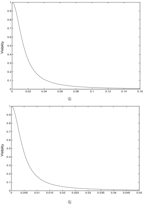
Figure 2: The visibility of interference fringes as a function of parametric gain, when the coincidence time window $T=1.8$ns and bandwidth of the light reaching the detectors is (a)1nm and (b)10nm

The visibility of the interference pattern as a function of the parametric gain, calculated from the expression for coincidence count rate in Eq. (37), is given by

$$V=\frac{A~{}cosh^{2}(|\xi|)}{A~{}cosh^{2}(|\xi|)+2~{}B~{}(\Delta T)~{}sinh^{2}(|\xi|)}$$ (38)

where $A$ and $B$ are constants arising from experimental factors. Fig. 2 shows plots of visibility as the bandwidth of light reaching the detectors is increased.

We now look into the features of the visibility plots and analyze the factors that give rise to these features. The important parameters for this purpose are the gain terms $cosh(|\xi|)$, $sinh(|\xi|)$ and $\Delta T$ in Eq. (37). The bandwidth $\Delta$ is a measure of the number of modes since we have assumed perfect phase matching. $\Delta T$ can be thought of as a measure of the detectors’ ability to resolve two entangled pairs of photons. A value of $\Delta T\gg 1$ leads to increase in accidental counts since detectors cannot distinguish every entangled pair of photons. The effect of the coincidence window time $T$ is easy to understand. In the very low gain limit ($sinh|\xi|)\approx 0$) only one single pair of entangled photons is produced within time $T$ and so every entangled pair can be distinguished. As the gain increases, many more entangled pairs are produced and reach the detectors within the coincidence window time causing accidental coincidences of photons belonging to different entangled pairs, and hence visibility is lost.

To understand the effect of the number of modes on the visibility, we go back to the output state of the OPA. The OPA state is restricted to include the two photon state and the next higher order interaction giving four photon states.

The output at the OPA, given in Eq. (13) can be written as

$$|\psi\rangle=\prod_{\vec{k}_{s}}exp[\frac{-\xi_{k_{s}}}{2}a^{\dagger}_{\vec{k}_{s}}(0)a^{\dagger}_{\vec{k}_{i}}(0)]|0\rangle$$ (39)

where $\vec{k}_{s}+\vec{k}_{i}=\vec{k}_{p}$ is the phase matching condition between the signal, idler and pump modes. We consider $n$ pairs of signal and idler modes, expand the exponential operator term in Eq. (39) and omit terms greater than second order in the gain parameter $\xi$. If the gain is considered constant for all the modes, then the unnormalized OPA state is given by

$$|\psi\rangle = |0\rangle-\left(\frac{|\xi|}{2}\right)\sum_{\vec{k}_{s}}|1_{\vec{k}_{s}}1_{\vec{k}_{i}}\rangle+$$

$$\left(\frac{|\xi|^{2}}{8}\right)\left[\sum_{\vec{k}_{s}}|2_{\vec{k}_{s}}2_{\vec{k}_{s}}\rangle+\sum_{\vec{k}_{s},\vec{k}^{{}^{\prime}}_{s}}|1_{\vec{k}_{s}}1_{\vec{k}_{i}}\rangle|1_{\vec{k}^{{}^{\prime}}_{s}}1_{\vec{k}^{{}^{\prime}}_{i}}\rangle\right]$$

From the expression for the truncated OPA state in Eq. (IV) we infer that the states in the first and second terms of the equation lead to ’good’ coincidence counts. The detectors detect photons belonging to a single entangled pair or to an entangled four photon state. The third term, on the other hand, can lead to detection of two photons belonging to different entangled states (’bad’ counts) half of the time. The conditional probability of getting a good count, given $n$ modes, is found to be

$$P(good|n)=\frac{16+(\frac{n+1}{2})\xi^{2}}{16+n\xi^{2}}$$ (41)

For a large number of modes, this probability tends to 0.5. This implies that when a large number of modes are allowed, the visibility of the coincidence detection pattern falls to 0.5.

Though the number of good counts seem to dominate according to Eq. (41), the number of modes along with the coincidence window time produce a loss in visibility greater than 0.5. As the gain increases the probability of both good and bad counts increase and tend towards a constant limit. This leads to the flattening of the visibility with rising parametric gain. The flattening of the visibility occurs at lower gain as the bandwidth(and number of modes)increases. The value of the limiting visibility falls as the number of allowed modes increases. This is to be expected since as the gain $\xi$ rises, entangled pairs (the first order states of the OPA) are emitted in all modes. If the number of modes allowed in the experiment are increased then the number of possible good and bad counts also increase. The coincidence time window $T$ further adds to the bad counts causing a greater fall in visibility and the limiting visibility is lowered.

If a smaller number of modes are allowed into the experiment, for example by using a fine pinhole, the visibility can be maintained at values greater than 0.5 for larger values of gain. But even in the case of just two modes, the visibility eventually falls due to the higher order states of the OPA and tends to a constant as $cosh(|\xi|)\approx sinh(|\xi|)\approx e^{|\xi|}/2$.

This is the fundamental difference in the mechanism of visibility loss with two-mode and multimode OPA. In a multimode OPA the loss of visibility is mainly due to the number of modes, and occurs at much lower gain than the two-mode OPA, where the higher order terms lead to loss of visibility for a given coincidence window time.

V Discussion and Summary

We have analyzed the effect of a multimode optical parametric amplifier source in the ’Ghost’ interference experiment, taking into account the finite coincidence window of the photon counting detectors. We find that the loss of visibility with increasing parametric gain is strongly dependent on the coincidence time window. A longer coincidence time window reduces the ability of the photon counting detectors to resolve entangled pairs as the parametric gain of the OPA increases. We have also highlighted the differences between effects observed with a two-mode and a multimode source. An increase in the number of modes in the experiment increases the probability of accidental coincidences between photons belonging to different entangled pairs (or states). Further, this experiment limited loss of visibility occurs in all coincidence counting measurements though it is significant only in the regime of a strong source of entangled photons like an OPA. We conclude that a cautious choice of sources and detection schemes are necessary in order to observe certain signatures of entangled light in a macroscopic regime.

Since the completion of this calculation we have become aware of a two-photon absorption technique demonstrated by Dayan et. al. Dayan where Rb atoms undergoing simultaneous absorption of signal and idler photons overcome the problem of temporal resolution associated with a strong broadband source like the multimode OPA. The two-photon transition is sensitive to minute delays (order of 100 fs) between the signal and idler photons. But such a detection scheme does not discriminate between entangled and separable pairs of photons and cannot reduce the loss of visibility in a ’Ghost’ interference experiment. Further, the use of such highly sensitive detection scheme requires a high gain OPA source which enhances accidental coincidence counts.

Appendix A Green’s Functions for propagation through a linear optical system

We give a brief review of propagation of an electric field through a diffraction limited linear optical system in each arm of the experimental set-up, following the treatment in  rubin . The positive frequency part of the electric field at a time $t$ at the input of a detector at $\vec{r}=z\hat{z}+\vec{\rho}$ is given by

$$E_{\beta}^{(+)}=\int\int d\omega d^{2}\vec{q}E(\omega)g(\vec{q},\omega,\vec{\rho},z)a_{\beta}(\omega,\vec{q})$$ (42)

where $a_{\beta}(\omega,\vec{q})$ is the annihilation operator at the source for a photon of angular frequency $\omega$, transverse wave vector $\vec{q}$ and polarization $\beta$. The unit vector $\hat{z}$ is the inward normal to the detector surface. $E(\omega)$ is a slowly varying function required for dimensional reasons and can be assumed constant in the current analysis. $g(\vec{q},\omega,\vec{\rho},z)$ is the optical transfer function or Green’s function which describes propagation through the linear optical system. In classical electromagnetic theory $g$ connects electric fields in real space. In our quantum mechanical analysis, it connects two operators in photon number or Fock space. The superposition principles involved in calculating $g$ are purely classical from classical electromagnetic theory. So in the quantum mechanical context it is best thought of as arising from boundary conditions on the modes of the fields irrespective of the state of the system.

We now calculate the Green’s function for the arm A in the Fig. (1). The Green’s function is expressed in terms of the aperture function defined by $t(\vec{\rho}_{a})$.

$$\begin{array}[]{l}g_{A}(\vec{q},\omega,0,d_{1}+d^{{}^{\prime}}_{1})=\\ \int d^{2}\rho_{a}\int d^{2}\rho_{s}h_{\omega}(-\vec{\rho}_{a},d^{{}^{\prime}}_{1})t(\vec{\rho}_{a})h_{\omega}(\vec{\rho}_{a}-\vec{\rho}_{s},d_{1})e^{i\vec{q}\cdot\vec{\rho}_{s}}\end{array}$$ (43)

where $\vec{\rho}_{s}$ and $\vec{\rho}_{a}$ are the transverse co-ordinates of the source (crystal) plane and aperture plane. In the Fresnel approximation goodman ,

$$h_{\omega}(\vec{\rho},d) = (\frac{-i\omega}{2\pi c})\frac{e^{i(\omega/c)d}}{d}\psi(|\vec{\rho}|,\frac{\omega}{cd})$$ (44)

$$\psi(|\vec{\rho}|,\frac{\omega}{cd}) = e^{i(\omega/2cd)\rho^{2}}$$ (45)

Finally

$$\begin{array}[]{l}g_{A}(\vec{q},\omega,0,d_{1}+d^{{}^{\prime}}_{1})=(\frac{-i\omega}{2\pi c})\frac{e^{i(\omega/c)(d_{1}+d^{{}^{\prime}}_{1})}}{d^{{}^{\prime}}_{1}}\\ \times\int d^{2}\rho_{a}\psi(|\vec{\rho}_{a}|,\frac{\omega}{cd^{{}^{\prime}}_{1}})t(\vec{\rho}_{a})e^{i\vec{q}\cdot\vec{\rho}_{a}}\psi(|\vec{q}|,-\frac{c}{\omega}d_{1})\end{array}$$ (46)

The Green’s function in the arm B of the experimental set-up, for each plane wave mode, assuming that the source has a large cross-section is given by

$$g_{B}(\vec{q},\omega,\vec{\rho},d_{2})=\int d^{2}\rho_{s}h_{\omega}(\vec{\rho}-\vec{\rho}_{s},d_{2})e^{i\vec{q}\cdot\vec{\rho}_{s}}$$ (47)

$$=e^{i(\omega/c)d_{2}}e^{i\vec{q}\cdot\vec{\rho}}\psi(|\vec{q}|,-\frac{c}{\omega}d_{2})$$ (48)

Using the above expressions for $g_{A}$ and $g_{B}$, we see that,

$$\begin{array}[]{l}\int d^{2}qg_{A}(-\vec{q},\omega,0,d_{1}+d^{{}^{\prime}}_{1})g_{B}(\vec{q},\omega,\vec{\rho},d_{2})=\\ (\frac{-i\omega}{2\pi c})\frac{e^{i(\omega/c)(d_{1}+d^{{}^{\prime}}_{1}+d_{2})}}{d^{{}^{\prime}}_{1}}\int d^{2}\rho_{a}\psi(|\vec{\rho}_{a}|,\frac{\omega}{cd^{{}^{\prime}}_{1}})t(\vec{\rho}_{a})\\ \times\int d^{2}qe^{i\vec{q}\cdot(\vec{\rho}-\vec{\rho}_{a})}\psi(|\vec{q}|,-\frac{c}{\omega}(d_{1}+d_{2}))\\ =-\left(\frac{\omega}{c}\right)^{2}\frac{e^{i(\omega/c)(d_{1}+d^{{}^{\prime}}_{1}+d_{2})}}{d^{{}^{\prime}}_{1}(d_{1}+d_{2})}\psi(|\vec{\rho}|,\frac{\omega}{c}\frac{1}{d_{1}+d_{2}})\\ \times\int d^{2}\rho_{a}\psi(|\vec{\rho}_{a}|,\frac{\omega}{c}(\frac{1}{d^{{}^{\prime}}_{1}}+\frac{1}{d_{1}+d_{2}}))e^{-i\frac{\omega}{c}\frac{1}{d_{1}+d_{2}}\vec{\rho}\cdot\vec{\rho}_{a}}t(\vec{\rho}_{a})\end{array}$$ (49)

In the far field Fraunhofer approximation, the $\psi$’s in the above expression go to unity and

$$\begin{array}[]{l}\int d^{2}qg_{A}(-\vec{q},\omega,0,d_{1}+d^{{}^{\prime}}_{1})g_{B}(\vec{q},\omega,\vec{\rho},d_{2})=\\ -\left(\frac{\omega}{c}\right)^{2}\frac{e^{i(\omega/c)(d_{1}+d^{{}^{\prime}}_{1}+d_{2})}}{d^{{}^{\prime}}_{1}(d_{1}+d_{2})}(2\pi)\tilde{t}(\frac{\omega}{c}\frac{\vec{\rho}}{d_{1}+d_{2}})\end{array}$$ (50)

where $\tilde{t}$ is the fourier transform of the aperture function. Further,

$$\begin{array}[]{l}|g_{A}|^{2}=\\ -(\frac{i\omega}{2\pi c})^{2}\frac{1}{d^{{}^{\prime}2}_{1}}\left[\int d^{2}\rho_{a}\psi(|\vec{\rho}_{a}|,\frac{\omega}{cd^{{}^{\prime}}_{1}})t(\vec{\rho}_{a})e^{i\vec{q}\cdot\vec{\rho}_{a}}\psi(|\vec{q}|,-\frac{c}{\omega}d_{1})\right]\\ \times\left[\int d^{2}\rho^{{}^{\prime}}_{a}\psi(|\vec{\rho}^{{}^{\prime}}_{a}|,\frac{\omega}{cd^{{}^{\prime}}_{1}})t(\vec{\rho}^{{}^{\prime}}_{a})e^{i\vec{q}\cdot\vec{\rho}^{{}^{\prime}}_{a}}\psi(|\vec{q}|,-\frac{c}{\omega}d_{1})\right]^{\ast}\end{array}$$ (51)

In the far- field Fraunhofer approximation,

$$|g_{A}|^{2} = (\frac{\omega}{2\pi c})^{2}\frac{1}{d^{{}^{\prime}2}_{1}}|\int d^{2}\rho_{a}t(\vec{\rho}_{a})e^{i\vec{q}\cdot\vec{\rho}_{a}}|^{2}$$ (52)

$$= (\frac{\omega}{2\pi c})^{2}\frac{1}{d^{{}^{\prime}2}_{1}}(2\pi)^{2}|\tilde{t}(\vec{q})|^{2}$$ (53)

Appendix B Singles Detection

We now look at results of detection at the detectors $D_{1}$ and $D_{2}$ individually, without caring for coincidences. This involves calculating the first order correlation functions glauber ,

$$G^{(1)}(\vec{r}_{i},t_{i})=\langle 0|E_{i}^{(-)}(\vec{r}_{i},t_{i})E_{i}^{(+)}(\vec{r}_{i},t_{i})|0\rangle$$ (54)

where $i=1,2$. Using the same techniques as in coincidence detection, we find that the first order correlation functions are given by

$$G_{A}^{(1)}(\vec{r}_{1},t_{1}) = \left(\frac{1}{2\pi}\right)^{3}\left(\frac{\omega_{p}}{4\pi cd^{{}^{\prime}2}_{1}}\right)^{2}\left(\frac{\hbar\omega_{p}}{4\epsilon_{0}c}\right)$$

$$\times sinh^{2}(|\xi|)\Delta\int d^{2}q_{o}|\tilde{t}(q_{o})|^{2}$$

$$G_{B}^{(1)}(\vec{r}_{2},t_{2}) = \left(\frac{1}{2\pi}\right)^{3}\left(\frac{\hbar\omega_{p}}{4\epsilon_{0}c}\right)\Delta sinh^{2}(|\xi|)$$

$$\times\int d^{2}q_{e}|g_{B}(\omega_{p}/2,\vec{q}_{e},\vec{\rho}_{2},d_{2})|^{2}$$

$G_{B}^{(1)}(\vec{r}_{2},t_{2})$ is the correlation function in the arm without the double slit and as expected, there is no interference pattern at $D_{2}$. The correlation function in the arm with the double-slit $G_{A}^{(1)}(\vec{r}_{1},t_{1})$, suggests that there might be a pattern at $D_{1}$, if the transverse components of the wave vector ($q_{o}$) reaching the detector is narrow enough. For the wavelengths and the dimensions of double-slit chosen, an interference pattern will be observed if the detection angle of the SPDC beam at the detector $\Delta\theta_{\perp}<2\lambda_{p}/a\approx 1.5$ mrad. But for the 1nm filter used, $\Delta\theta_{\perp}\approx 15$ mrad. Therefore, no interference pattern is found behind the double slit due to the large divergence of the SPDC beam.

References

• (1) D. V. Strekalov, A. V. Sergienko, D. N. Klyshko and Y. H. Shih, Phys. Rev. Lett. $\bf{74}$, 3600 (1995).
• (2) E. M. Nagasako, S. J. Bentley, R. W. Boyd, G. S. Agarwal, Phys. Rev.A $\bf{64}$, 043802 (2001).
• (3) A. Gatti, E. Brambilla, M. Bache and L. A. Lugiato, quant-ph/0307187.
• (4) M. Bache, E. Brambilla, A. Gatti and L. A. Lugiato, quant-ph/0402160.
• (5) T.B. Pittman et. al., Phys. Rev. A 52, R3429 (1995); T.B. Pittman et. al., Phys. Rev. A 53, 2804 (1996)
• (6) B. R. Mollow, R. J. Glauber , Phys. Rev. $\bf{160}$, 1097 (1967); $\bf{162}$, 1256 (1967).
• (7) R.J. Glauber, Phys. Rev. 130 (1963) 2529; 131 (1963) 2766.
• (8) D.N. Klyshko, Photon and Nonlinear Optics, Gordon and Breach Science, New York, (1988).
• (9) W. H. Louisell, A. Yariv and A. E. Siegman, Phys. Rev. $\bf{124}$, 1646 (1961).
• (10) M. O. Scully and M. S. Zubairy, Quantum Optics, Cambridge University Press, NewYork, (1997).
• (11) D. F. Walls and G. J. Milburn, Quantum Optics, Springer-Verlag, NewYork, (1994).
• (12) M. Born and E. Wolf, Principles of Optics, 6th ed., Pergammon Press, Oxford, (1980).
• (13) M. H. Rubin, Phys. Rev. A $\bf{54}$, 5349 (1996).
• (14) A. Yariv, Quantum Electronics, John Wiley $\&$ Sons Inc., (1989).
• (15) Z. Y. Ou and L. Mandel, Phys. Rev. Lett, $\bf{61}$, 50 (1988).
• (16) B. Dayan, A. Pe’er, A. A. Friesem and Y. Silberberg. Phys. Rev. Lett $\bf{93}$, 023005 (2004)
• (17) J. W. Goodman, Introduction to Fourier Optics, McGraw-Hill Publishing Company, NewYork, (1968).