Multi-splitter interaction for entanglement distribution

Abstract

In protocols of distributed quantum information processing, a network of bilateral entanglement is a key resource for efficient communication and computation. We propose a model, efficient both in finite and infinite Hilbert spaces, that performs entanglement distribution among the elements of a network without local control. In the establishment of entangled channels, our setup requires only the proper preparation of a single elected element. We suggest a setup of electromechanical systems to implement our proposal.

The role of entanglement in delocalized architectures of a device for quantum information processing (QIP) has been investigated under many aspects varie0 . Entanglement between distant sites of a distributed register is a fundamental requisite to optimize communication protocols and perform efficient quantum computation varie . In this context, an entanglement distributor creates an entangled network of the elements of a register that, otherwise, have no direct reciprocal interaction. The efficiency of the distributor can be quantified by the number of elements which are entangled per single use of the distributor or by the amount of entanglement shared by any two of them. Thus, the choice of the most appropriate design of the distributor is a problem-dependent issue with no general recipe. An interesting configuration for this problem is a star-shaped system in which an elected element interacts simultaneously with many other independent subsystems huttonbose .

In this paper, we propose a model that acts as an efficient entanglement distributor. An important feature of our proposal is that no local control on the dynamic of the participating systems is required once the interactions are set. We only need the pre-engineering of the network and a proper control of the interaction time. This is an advantage exploitable in those situations (frequent in solid-state physics) where single-element addressing is hard or impossible. The interaction we suggest acts on a multipartite bosonic network whose evolution can be tracked analytically both in the discrete and the continuous variable (CV) case.

Despite our proposal being naturally described using the quantum optics language, we show that our model is general enough to find interesting applications in solid-state physics. We sketch a system of coupled electromechanical oscillators to embody our model. Similar setups have recently found applications in the entanglement-transmission problem plenio .

The model - We consider $N$ bosons (or modes) $b_{j}$ ($j=1,..,N$) described by the annihilation (creation) operators $\hat{b}_{j}$ ($\hat{b}^{\dagger}_{j}$) and an additional mode, labeled $a$, which we call the ${\it root}$. The interaction configuration is sketched in Fig. 1 (a) and consists of the resonant couplings of the root to each $b_{j}$. The satellite elements $b_{j}$ do not mutually interact. In the interaction picture, we consider the Hamiltonian

$$\hat{H}_{I}=\sum^{N}_{j=1}\mathcal{G}_{j}\hat{a}^{{\dagger}}\hat{b}_{j}+h.c.\hskip 14.22636pt(\hbar=1)$$ (1)

with $\mathcal{G}_{j}$ real and time-independent couplings.

(a)                                   (b)

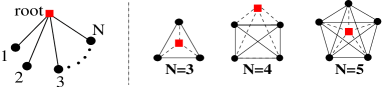
Figure 1: (a): The interaction configuration in Eq. (1). Each edge represents an interaction. (b): Complete entanglement graph generated by Eq. (1). Solid and dashed edges represent entanglement.

For $N=1$, $\hat{U}(\tau)=e^{-i\hat{H}_{I}\tau}$ is similar to a beam-splitter (BS) superimposing mode $a$ to $b_{1}$. We analyze the characteristics of the many-body dynamics corresponding to $N>1$. After a lengthy calculation based on Lie algebra we find that $\hat{U}(\tau)$ can be decomposed as

$$\hat{U}(\tau) =\left[\otimes^{N-1}_{j=1}\hat{R}_{b_{j}}\hat{B}_{b_{j+1}b_{j}}(\varepsilon_{j},0)\right]\hat{B}_{b_{N}a}(\vartheta_{N}\tau,-{\pi}/{2})$$ (2)

$$\otimes\left[\otimes^{N-1}_{j=1}\hat{R}_{b_{N-j}}\hat{B}_{b_{N-j+1}b_{N-j}}(\varepsilon_{N-j},0)\right],$$

where $\vartheta^{2}_{k}=\sum^{k}_{j=1}{\cal G}^{2}_{j}$. $\hat{R}_{b_{j}}=e^{i\pi\hat{b}^{\dagger}_{j}\hat{b}_{j}}$ is a $\pi$-phase shifter for mode $b_{j}$, $\varepsilon_{j}=\cos^{-1}({\cal G}_{j+1}/\vartheta_{j+1})$ and $\hat{B}_{ab}(v,\varphi)=e^{[v(\hat{a}^{\dagger}\hat{b}e^{i\varphi}-\hat{a}\hat{b}^{\dagger}e^{-i\varphi})]}$ denotes a BS operator. This decomposition is extremely useful as it shows that the dynamic can be interpreted as the action of a setup of optical elements on $N+1$ bosons. Eq. (2) describes how the root gains information from $b_{j}$’s via the interaction $\hat{B}_{b_{N}a}$ as well as the distribution of any information initially in $a$ to the satellites. The form of Eq. (2) reveals that, if $b_{j}$’s are all prepared in rotationally-invariant states (such as $|0\rangle$ or thermal states), the transformations prior to $\hat{B}_{b_{N},a}$ do not contribute to the entanglement dynamics myungBS . By properly setting the $\varepsilon_{j}$, the evolution of the network can be made equivalent to an array of BS’s which sequentially superimpose $a$ to $b_{j}$ modes. If $a$ is in a superposition of $\left|0\right\rangle$ and a coherent state, $b_{j}$’s being in the vacuum state, we generate an $(N+1)$-mode GHZ state useful for secret sharing hillery . The entire Eq. (2) must be considered if we initially prepare one or more satellite modes in a coherent or a non-classical state.

The model described by Eq. (1) realizes various interference patterns in the equivalent all-optical setting allowing for different tasks. For instance, if ${\cal G}_{j}={\cal G}$ ($\forall{j}$), $\hat{H}_{I}$ describes an effective $XY$-coupling suitable for $1\rightarrow{N}$ phase-covariant cloning clone . As another example, let us take $N=2$ so that Eq. (2) reduces to $\hat{U}(\tau)=\hat{R}_{b_{1}}\hat{B}_{b_{2}b_{1}}(\varepsilon_{1},0)\hat{B}_{b_{2}a}(\sqrt{2}{\cal G}\tau,-\pi/2)\hat{R}_{b_{1}}\hat{B}_{b_{2}b_{1}}(\varepsilon_{1},0)$ with $\varepsilon_{1}=\pi/4$. We assume that mode $b_{1}$ is initially prepared in the single-excitation state $\left|1\right\rangle_{b_{1}}$, $b_{2}$ and $a$ being in the vacuum (the investigation can be generalized to the case of $b_{1}$ being prepared in a coherent state). It is easily seen from our decomposition that at $\sqrt{2}{\cal G}\tau={\pi}$, the initial state is transferred to mode $b_{2}$ with unit probability (while the maximum probability of finding the initial state in $a$ is only $1/2$). This analysis shows that perfect quantum state transfer from $b_{1}$ to $b_{2}$ can be performed through mode $a$. In fact, when $\sqrt{2}{\cal G}\tau=n\pi$ ($n=0,1,\cdots$), it is interesting to note that our model is equivalent to a Mach-Zehnder interferometer with a $n\pi$ phase-shift in the path of mode $b_{2}$, which is obvious from our decomposition in Eq. (2).

Single excitation case - Consider $a$ initially prepared in $\left|1\right\rangle_{a}$, $b_{j}$’s being in $\otimes^{N}_{j=1}\left|0\right\rangle_{j}$. The dynamics is captured by considering a fictitious collective mode of its annihilation operator $\hat{c}=\sum^{N}_{j=1}{\cal G}_{j}\hat{b}_{j}/\vartheta_{N}$. Thus, $\hat{U}(\tau)\left|10..0\right\rangle_{ab_{1}..b_{N}}=\cos(\vartheta_{N}\tau)\left|1\underline{0}\right\rangle_{ac}-i\sin(\vartheta_{N}\tau)\left|0\underline{1}\right\rangle_{ac}$ with $\left|\underline{1}\right\rangle_{c}=\hat{c}^{{\dagger}}\left|0..0\right\rangle_{b_{1}..b_{N}}=\sum_{j}({\cal G}_{j}/\vartheta_{N})\left|0..1..0\right\rangle_{b_{1}..b_{j}..b_{N}}$. This state can be pictorially described by complete entanglement graphs as those shown in Fig. 1 (b). There, solid or dashed edges represent entanglement.

In the basis $\{\left|00\right\rangle,\left|01\right\rangle,\left|10\right\rangle,\left|11\right\rangle\}_{b_{i}b_{j}}$, the reduced density matrix of the generic pair $b_{i},\,b_{j}$ ($\forall\,i,j$) reads

$$\bm{\rho}_{{i}{j}}=\begin{pmatrix}1-(G^{2}_{iN}+G^{2}_{jN})&0&0&0\\ 0&G^{2}_{jN}&G_{iN}G_{jN}&0\\ 0&G_{iN}G_{jN}&G^{2}_{iN}&0\\ 0&0&0&0\end{pmatrix},$$ (3)

where $i<j$ and $G_{jN}={\cal G}_{j}\sin(\vartheta_{N}\tau)/\vartheta_{N}$. The entanglement of this mixed state can be quantified by the concurrence $C_{N}=\max\left\{0,{\alpha_{1}}-{\alpha_{2}}-{\alpha_{3}}-{\alpha_{4}}\right\}$ concurrence . Here, $\alpha_{i}$’s are the square roots of the eigenvalues (in non-increasing order) of $\bm{\rho}_{ij}(\bm{\sigma}_{y}\otimes\bm{\sigma}_{y})\bm{\rho}^{*}_{ij}(\bm{\sigma}_{y}\otimes\bm{\sigma}_{y})$ with $\bm{\rho}^{*}_{ij}$ the complex conjugate of $\bm{\rho}_{ij}$ and $\bm{\sigma}_{y}$ the $y$-Pauli matrix. We get $C_{N}=\max\{0,2G_{iN}G_{jN}\}$. For later purposes, it is also useful to consider the entanglement measure based on negativity of partial transposition (NPT) npt . NPT is a necessary and sufficient condition for entanglement of any bipartite qubit state npt . The corresponding entanglement measure is defined as $NPT_{N}=\max\{0,-2\lambda^{-}\}$ with $\lambda^{-}$ the negative eigenvalue of $\bm{\rho}^{T_{j}}_{ij}$ which is the partial transposition of $\bm{\rho}_{ij}$ with respect to $b_{j}$. We find ${NPT}_{N}=\max\{0,{[(1-G^{2}_{iN}-G^{2}_{jN})^{2}+4G^{2}_{iN}G^{2}_{jN}]^{1/2}}-(1-G^{2}_{iN}-G^{2}_{jN})\}$. $C_{N}$ and $NPT_{N}$ are optimized when $\vartheta_{N}\tau=(2k+1)\pi/2$ ($k\in{\mathbb{Z}}$). Using this condition as a constraint in the Lagrange’s method of indeterminate multipliers, we find that $C_{N}$ and $NPT_{N}$ are maximized for the uniform set of couplings ${\cal G}_{j}={\cal G}$ ($\forall{j}$). In this case we get $C_{N,max}=2/N$ and $NPT_{N,max}=\{[{4+(N-2)^{2}}]^{1/2}-(N-2)\}/N$. $2/N$ is the upper bound for the bipartite entanglement in an $N$-party system buzekimoto . Thus, Eq. (1) is optimal under the point of view of pairwise entanglement distribution. For equal ${\cal G}_{j}$, the $\bm{\rho}_{ij}$ are all equal and we have $\left|10..0\right\rangle_{ab_{1}..b_{N}}{\rightarrow}\cos(\vartheta_{N}\tau)\left|1,0..0\right\rangle_{ab_{1}..b_{N}}-i\sin(\vartheta_{N}\tau)\left|0,W_{N}\right\rangle_{ab_{1}..b_{N}}$. We have introduced the $N$-particle $W$-state $\left|W_{N}\right\rangle_{b_{1}..b_{N}}=N^{-1/2}\sum_{j}\left|0..1..0\right\rangle_{b_{1}..b_{j}..b_{N}}$ which is the state achieving $C_{N,max}$buzekimoto . Thus, the maximum concurrence between any pair of $b_{j}$’s is found when the root is separable from the rest of the network. The corresponding graph is obtained by deleting the dashed edges in Fig. 1 (b), the satellite elements forming complete and permutation-invariant entanglement graphs. The system periodically evolves from a separable state to a configuration where the root is factorized from the rest of the network (which is in $\left|W_{N}\right\rangle_{b_{1}..b_{N}}$). In between, an ($N+1$)-partite entangled state is obtained.

Recently, a configuration of many spin-$1/2$ systems analogous to Eq. (1) has been proposed huttonbose . The one-excitation case we have considered allows for a comparison between the two situations, both achieving $C_{N,max}=2/N$. In our model the bosonic nature of the register allows for this result without local control on the satellite elements or the root. In ref. huttonbose , on the other hand, this is obtained by using an additional magnetic interaction and through the measurement of the state of the root.

In order to further characterize our entanglement distributor, we compare $\left|W_{N}\right\rangle_{b_{1}..b_{N}}$ to the class of cluster states. These are known to be useful and genuine multipartite entangled states cluster , inequivalent to $\left|W_{N}\right\rangle$ for any $N$. While there are always proper local measurements on a subset of a cluster that allow for the deterministic extraction of a pure Bell state, this is not the case for a $W$-state. However, the quantum correlations in a cluster are encoded in the system as a whole and any pairwise entanglement (obtained by tracing out the rest of the cluster) is zero. This is a drawback in those situations where bipartite entanglement is required but the physical system is such that the realization of a measurement pattern is made difficult by the problems related to single-element addressing. Finally, the entanglement of $\left|W_{N}\right\rangle$ is persistent as $N-1$ projective measurements are required in order to disentangle the elements of the register. For the problem we address here, our analysis shows that Eq. (1) is a suitable and exploitable model.

CV case - Considering only the case of a single excitation in the root restricts the possibilities offered by the bosonic nature of our register. In ref. myungBS it is shown that a non-classical input is a fundamental pre-requisite for the entanglement of the outputs of a beam-splitter. The same is true in our case because of the analogy between a BS and Eq. (2). On the other hand, necessary and sufficient conditions for the entanglement are known and entanglement can be quantitatively determined only for the class of two-mode CV Gaussian states simon ; myungmunro . In virtue of these considerations and because of the Gaussian-preserving nature of the linear operations in (2), only Gaussian states will be considered here.

A powerful tool in the analysis of $N$-mode CV systems is given by the variance matrix $\bf{V}$, defined (after unitary displacements) as $V_{\alpha\beta}=\langle\{\hat{x}_{\alpha},\hat{x}_{\beta}\}\rangle\,(\alpha,\beta=1,..,N)$. Here, ${\bf\hat{x}}=(\hat{q}_{1},\hat{p}_{1},..,\hat{q}_{N},\hat{p}_{N})^{T}$ is the vector of the quadratures. A Gaussian state is fully characterized by the knowledge of just the first and second moments of ${\bf\hat{x}}$ and, in order to characterize the state of our $N+1$ modes, we need to find the variance matrix of their joint state after $\hat{U}(\tau)$. In phase-space, the action of $\hat{U}(\tau)$ is such that ${\bf V^{\prime}}={\cal T}^{T}{\bf V}{\cal T}$ becomes the new variance matrix. Here, ${\cal T}$ is the $2(N+1)\times{2(N+1)}$ unitary matrix (found using Eq. (2))

$${\cal T}=\begin{pmatrix}\cos{(\vartheta_{N}\tau)}\mbox{$1{\bf l}$}_{2}&A_{1}{\bm{\sigma}}_{y}&A_{2}{\bm{\sigma}}_{y}&\cdots&A_{N}{\bm{\sigma}}_{y}\\ A_{1}{\bm{\sigma}}_{y}&D_{11}\mbox{$1{\bf l}$}_{2}&D_{12}\mbox{$1{\bf l}$}_{2}&\cdots&D_{1N}\mbox{$1{\bf l}$}_{2}\\ \vdots&\cdots&\cdots&\ddots&\vdots\\ A_{N}{\bm{\sigma}}_{y}&D_{N1}\mbox{$1{\bf l}$}_{2}&D_{N2}\mbox{$1{\bf l}$}_{2}&\cdots&D_{NN}\mbox{$1{\bf l}$}_{2}&\end{pmatrix},$$ (4)

where $\mbox{$1{\bf l}$}_{2}$ is the 2$\times$2 identity matrix, $A_{n}=-iG_{nN}$ and $D_{nm}=\delta_{nm}+[{\cal G}_{n}{\cal G}_{m}(\cos(\vartheta_{N}\tau)-1)/\vartheta^{2}_{N}]$. $\delta_{nm}$ denotes the Kronecker symbol.

For simplicity, we take ${\cal G}_{j}={\cal G}$ ($\forall{j}$), $b_{j}$’s being in the vacuum state (variance matrix ${\bf V}_{b_{1}..b_{N}}=\oplus^{N}_{j=1}\mbox{$1{\bf l}$}_{2b_{j}}$). The root is prepared in a squeezed state (squeezing parameter $r$) which is the most natural non-classical Gaussian state myungBS . The initial variance matrix of the system is ${\bf V}_{a}\oplus{\bf V}_{b_{1}..b_{N}}$ with ${\bf V}_{a}\equiv{e}^{-r\bm{\sigma}_{z}}$ the variance matrix of $a$ and $\bm{\sigma}_{z}$ is the $z-$Pauli matrix. By tracing all the modes but $b_{i}$ and $b_{j}$ we get

$${\bf V^{\prime}}_{b_{i}b_{j}}=\begin{pmatrix}{\bf L}_{N}&{\bf C}_{N}\\ {\bf C}_{N}&{\bf L}_{N}\end{pmatrix}.$$ (5)

Here, ${\bf L}_{N}\!=\!\mbox{diag}(n_{N},m_{N}),\,{\bf C}_{N}\!=\!\mbox{diag}(c_{N},d_{N})$ with $n_{N}=1+c_{N}$, $m_{N}=1+d_{N}$, $c_{N}=-e^{r}d_{N}=(e^{r}-1)\sin^{2}(\vartheta_{N}\tau)/N$. No dependence on the indices $i,j$ exists so that Eq. (5) is the same for any pair. ${\bf V^{\prime}}_{b_{i}b_{j}}$ has a form which allows us to quantify the bipartite entanglement. Indeed, for a variance matrix as Eq. (5), the NPT entanglement measure is given by ${\cal E}_{N}=\max\{0,(\delta_{1}\delta_{2})^{-1}-1\}$ with $\delta_{1}=n_{N}-\left|c_{N}\right|$ and $\delta_{2}=m_{N}-\left|d_{N}\right|$ myungmunro . We have

$${\cal E}_{N}=\max\left\{0,\frac{2(1-e^{-r})\sin^{2}(\vartheta_{N}\tau)}{N-2(1-e^{-r})\sin^{2}(\vartheta_{N}\tau)}\right\},$$ (6)

which is plotted in Fig. 2 (a) against the effective coupling $g={\cal G}\tau$.

(a)                                   (b)

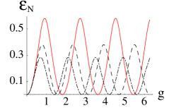
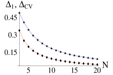
Figure 2: (a): ${\cal E}_{N}$ against the dimensionless time $g={\cal G}\tau$ for $N=3$ (solid line), $N=4$ (dashed line) and $N=5$ (dot-dashed). The squeezing of the initial root state is $r=0.8$. (b): Relative entanglement differences $\Delta_{1}$ ($\bigstar$) and $\Delta_{CV}$ ($\blacklozenge$) against $N$.

${\cal E}_{N}$ diminishes as $N$ increases and, for fixed values of $r$, is maximized at $\vartheta_{N}\tau=(2k+1)\pi/2$ ($k\in{\mathbb{Z}}$). In Fig. 2 (a) only ${\cal E}_{N\geq{3}}$ is shown as $N=2$ requires some comments. For this particular case, by generalizing the results of the analysis in refs. myungBS ; referee , we expect the evolved state of modes $b_{1},\,b_{2}$ to be locally equivalent to a two-mode squeezed vacuum. This result is crucially dependent on the fact that, from Eq. (2) for $N=2$ and $\vartheta_{2}\tau=\pi/2$, the interaction between the satellite modes is an effective $50:50$ BS. This allows us to decompose the variance matrix of the resulting two-mode state as ${\bf V^{\prime}}_{b_{1}b_{2}}={O}(\frac{-r}{4}){\bf S}_{b_{1}b_{2}}(\frac{r}{4}){O}(\frac{-r}{4})$. Here $O(\frac{-r}{4})=\otimes^{N}_{j=1}{\bf S}_{b_{j}}(\frac{-r}{4})$ with ${S}_{b_{j}}$ the single-mode squeezing transformation (which does not modify the entanglement structure) and ${\bf S}_{b_{1}b_{2}}(\frac{r}{4})$ the variance matrix of a two-mode squeezed vacuum myungmunro . The state is pure which implies the separability of $a$ from $b_{1}+b_{2}$. By studying the purity ${\cal P}_{b_{1}b_{2}}={[\det{\bf V^{\prime}}_{b_{1}b_{2}}]}^{-\frac{1}{2}}$ myungmunro , we find that its period is one-half the period of ${\cal E}_{2}$. That is, the $b_{1}+b_{2}$ state is pure not only when ${\cal E}_{2}$ is maximum (at $\tau_{odd}=(2k+1)\pi/(2\sqrt{2}{\cal G})$) but also at $\tau_{even}=k\pi/(\sqrt{2}{\cal G})$, which corresponds to ${\cal E}_{2}=0$. By using the biseparability condition of a boson from a group of $N$ others ww , we have also checked that at $\tau_{even}$ no entanglement is found between $a$ and $b_{1}+b_{2}$. The state is fully separable.

By enlarging the network to $N\geq{3}$, we notice that the first interaction in Eq. (2) between two satellite modes is a BS of its $\varepsilon_{N-1}=1/\sqrt{N}$, which is no longer a $50:50$ BS. This stops the possibility of getting a state locally equivalent to a two-mode squeezed state spiegazione and the structure of the multi-mode entangled state becomes much more complicated than the simple case of $N=2$. In particular, the state of any pair $(b_{i},b_{j})$ is pure just at $g_{even}$ but no longer when ${\cal E}_{N}$ is maximum. Thus, quantum correlations are shared between $b_{j}$’s at $\tau_{odd}=(2k+1)\pi/(2\sqrt{N}{\cal G})$ but not between the root and them. The entanglement configuration alternates between a fully separable state and a many-body entangled state of just $b_{j}$’s, passing by a configuration in which entanglement is shared with $a$. The picture given by the graphs in Fig. 1 (b) is still valid.

We now look at the effect of increasing $N$ on the properties on the entanglement distribution. We consider the quantities $\Delta_{1}=1-(NPT_{N+1,max}/NPT_{N,max})$ and $\Delta_{CV}=1-({\cal E}_{N+1,max}/{\cal E}_{N,max})$ which measure the relative loss in pairwise entanglement if the network is enlarged by one element. Fig. 2 (b) shows that at a fixed $r$, $\Delta_{1}$ and $\Delta_{CV}$ decrease with $N$ ($3\leq{N}\leq{20}$). The distribution process is only weakly affected and the entanglement is still spread through the network. In passing, it is interesting to stress the qualitative robustness of the distributed entanglement in the CV case as compared to the discrete one, an issue which, in a different context, has also been noticed in wvc .

Possible setups - We briefly mention that, to embody Eq. (1), we can use the interaction of a linearly polarized optical bus with $N$ ensembles of cold atoms (confined in vapor cells), providing the Hamiltonian $\hat{H}_{le}=\kappa\hat{p}_{ph}\sum^{N}_{i=1}\hat{p}_{ei}$ ($\kappa$ is a coupling rate). Here, $\hat{p}_{ph}$ ($\hat{p}_{ei}$) is the momentum operator of the bus ($i^{th}$ atomic ensemble) whose wavelength is assumed to be much larger than the dimensions of the ensembles and their separations polzik . $\hat{H}_{le}$ holds within the Stokes-vector formalism for the bus and the Holstein-Primakoff transformation mapping collective states of an ensemble into a fictitious boson. By discarding rapidly-oscillating terms, $\hat{H}_{le}\rightarrow\hat{H}_{I}$.

Stimulating opportunities come from micro and nano-electromechanical systems (MEMS and NEMS), i.e. electrically controlled mechanical oscillators (or cantilevers) whose dimensions are in the range from $10^{-9}$ to $10^{-6}\,m$. Doubly clamped cantilevers with fundamental mode frequency in the range of $[10^{7}-10^{9}]\,Hz$ have been fabricated and mutually coupled buks . They are useful to study Heisenberg-limited measurements knobel and entanglement plenio ; armour . There are theoretical proposals for ground-cooling and squeezing of NEMS mode zoller . The preparation of phonon-number states and the tomography of a vibrational mode have also been addressed zoller .

We consider $N$ classical oscillators coupled via spring-forces to a central one, the analogue of our root. Within Hooke’s law, the energy of the system is ${\cal H}=(\omega/2)(q^{2}_{a}+p^{2}_{a})+(\omega/2)\sum_{j}[q^{2}_{j}+p^{2}_{j}+{\cal K}_{j}(q_{j}-q_{a})^{2}]$, where the ${\cal K}_{j}$’s are the coupling factors, $(q_{j},\,p_{j})$ are proper canonical variables and $\omega$ is the frequency of the oscillators (equal for all). Each ${\cal K}_{j}$ is controlled via voltage biases between the cantilevers. Each bias creates a potential that changes with the capacitance between two oscillators. Eq. (1) is then found in a second-quantization picture and within the rotating wave approximation (used for ${\cal K}_{i}\simeq 0.1{\omega}$). The oscillators can be built via photolitography of gold on silicon substrates buks . In our case, planar grids of a few cantilevers face each other in pairs, surrounding the root. The coupling of the cantilevers to the phononic modes of the substrate is the main source of decoherence. However, oscillators with quality factors $Q\simeq{10}^{4}$ and $\omega\simeq{10}\,MHz$ (coherence times $\simeq 1$ msec) allow now for a good number of coherent operations. The reconstruction of ${\bf V}^{\prime}_{b_{i}b_{j}}$ is challenging here. However, a single-electron-transistor (SET) capacitively coupled to the cantilevers can be used armour . Exploiting the changes of the coupling capacitances (which depend on the instantaneous position of the oscillators), a SET acts as a displacement-to-current transducer with displacement sensitivity $\simeq 10^{-16}\,m/\sqrt{{Hz}}$. Stroboscopic techniques to infer ${\bf V}^{\prime}_{b_{i}b_{j}}$ could then be used plenio .

Remarks - We have characterized a many-body interaction that, through just global interaction with a seeding system, distributes entanglement in a network of local processors. The dynamics is described by linear operations and the model is flexible enough to allow for different interference patterns by pre-engineering the couplings and the initial state. We have shown how symmetric bipartite entangled states are generated both in the discrete and CV case. To embody our model, we have described a setup of coupled cantilevers that offers nice perspectives in the study of entanglement distributors for QIP.

- (1) D. Gottesman and I.L. Chuang, Nature (London) 402, 390 (1999); L.-M. Duan et al., ibid. 414, 413 (2001).
- (2) J. Eisert et al., Phys. Rev. A 62, 52317 (2000).
- (3) A. Hutton and S. Bose, Phys. Rev. A 69, 042312 (2004).
- (4) J. Eisert et al., Phys. Rev. Lett. (to appear) (2004); M.B. Plenio and F.L. Semio, quant-ph/0407034; M.B. Plenio et al., New J. Phys. 6, 36 (2004).
- (5) M.S. Kim et al., Phys. Rev. A 65, 032323 (2002).
- (6) M. Hilllery et al., Phys. Rev. A 59, 1829 (1999).
- (7) G. De Chiara et al., Phys. Rev. A (to appear) (2004).
- (8) W.K. Wootters, Phys Rev. Lett. 80, 2245 (1998).
- (9) A. Peres, Phys. Rev. Lett. 77, 1413 (1996); M. Horodecki, et al., Phys. Lett. A 223, 1 (1996).
- (10) M. Koashi, et al., Phys. Rev. A 62, 050302 (2000).
- (11) H.J. Briegel and R. Raussendorf, Phys. Rev. Lett. 86, 910 (2001).
- (12) R. Simon, Phys. Rev. Lett. 84, 2726 (2000).
- (13) M.S. Kim et al., Phys. Rev. A 66, R030301 (2002).
- (14) Z. Y. Ou, et al., Phys. Rev. Lett. 68, 3663 (1992); Z.Y. Zou et al., Appl. Phys. B 55 265 (1992).
- (15) C. Schori et al., Phys. Rev. Lett. 89, 057903 (2002).
- (16) R. Werner and M. Wolf, Phys. Rev. Lett. 86, 3658 (2001).
- (17) This is a consequence of the inequality holding for . denotes single-mode squeezing.
- (18) M.M. Wolf, et al., Phys. Rev. Lett. 92, 087903 (2004).
- (19) E. Buks and M.L. Roukes, JMEMS 6, 1057 (2002).
- (20) R.G. Knobel et al., Nature (London) 424, 291 (2003).
- (21) A.D. Armour et al., Phys. Rev. Lett. 88, 148301 (2002).
- (22) I. Martin et al., Phys. Rev. B 69, 125339 (2004).