Tracing the bounds on Bell-type inequalities

Abstract

Bell-type inequalities and violations thereof reveal the fundamental differences between standard probability theory and its quantum counterpart. In the course of previous investigations ultimate bounds on quantum mechanical violations have been found. For example, Tsirelson’s bound constitutes a global upper limit for quantum violations of the Clauser-Horne-Shimony-Holt (CHSH) and the Clauser-Horne (CH) inequalities. Here we investigate a method for calculating the precise quantum bounds on arbitrary Bell-type inequalities by solving the eigenvalue problem for the operator associated with each Bell-type inequality. Thereby, we use the min-max principle to calculate the norm of these self-adjoint operators from the maximal eigenvalue yielding the upper bound for a particular set of measurement parameters. The eigenvectors corresponding to the maximal eigenvalues provide the quantum state for which a Bell-type inequality is maximally violated.

I Introduction

One of the most puzzling features of quantum mechanics is the violation of so-called Bell-type inequalities representing a cornerstone of our present understanding of quantum probability theory peres93 . As pointed out by John Bell bell64 such a violation, as predicted by quantum mechanics, requires a radical reconsideration of basic physical principles like the assumption of local realism. However, Bell-type inequalities have already a long tradition dating back to George Boole’s work on “conditions of possible experience” boole54 ; boole62 , dealing with the question of necessary and sufficient conditions on probabilities of logically interconnected events . Take for example the statements: “The probability of rain in Växjö is about $80\%$” and “The probability of rain in Vienna is $90\%$”. Nobody would believe that the joint probability of rain in both places could be just $10\%$ — the claim that the joint probability is very much lower than the single probabilities is apparently counterintuitive. The question remains: Which numbers could be considered reasonable and consistent? Boole’s requirements on the (joint) probabilities are expressed by certain equations or inequalities relating those (joint) probabilities.

Since Bell’s investigations bell64 ; bell66 into bounds on classical probabilities and their relation to quantum mechanical predictions, similar inequalities for particular physical setups have been discussed in great number and detail (see for example Refs. clauser69 ; clauser74 ; werner-wolf01 ; zukowskibrukner02 ). Furthermore, violations of Bell-type inequalities, as predicted by quantum mechanics, have been experimentally verified in different areas of physics aspect82 ; weihs98 ; rowe01 ; hasegawa03 to a very good degree of accuracy.

However, whereas these bounds are interesting for an inspection of the violations of classical probabilities by quantum probabilities, the issue of the validity of quantum probabilities and their experimental verification is completely different. Recently, Bovino et al. bovino04 conducted an experiment based on numerical studies by the current authors filipp-svozil04 and triggered by a proposal of Cabello cabello04 to verify bounds on quantum probabilities depending on a particular choice of measurements.

In what follows we shall present analytical as well as numerical studies on such quantum bounds allowing for further experimental tests of different kinds of Bell-type inequalities.

II Correlation Polytopes

At first we shall start from a geometrical derivation of bounds on classical probabilities given by linear inequalities in terms of correlation polytopes froissart81 ; pitowsky89 ; pitowsky01a ; pitowsky94 ; tsirelson80 . Considering an arbitrary number of classical events $a_{1},a_{2},\ldots,a_{n}$ one can assign to each event a certain probability $p_{1},\,p_{2},\,\ldots,\,p_{n}$ and probabilities $p_{12},\ldots$ for the joint events $a_{1}\cap a_{2},\ldots$. These probability values can be collected to form the the components of a vector $p=(p_{1},p_{2},\ldots,p_{n},p_{12},\ldots)$, where each $p_{i},\,p_{ij}\ (i,j=1,\ldots,n)$ can take values in the interval $[0,1]$. Since the events $a_{1},\,a_{2},\,\ldots$ are assumed to be independent, each single probability $p_{i}$ can also take its extremal value $0$ or $1$ and the vectors comprising all possible combinations of extremal values ($p_{i}=0,1$ and $p_{ij}=p_{i}p_{j}$) can be regarded as rows of a truth table; with the symbols “$0$” and “$1$” corresponding to “false” and “true,” respectively.

Any classical probability distribution; i. e., any vector $p$, can be represented as a convex sum over the extremal probability distributions given by the row entries of the truth table. It can therefore be regarded as some point $p\in C$ where $C={\textrm{c}onv}(K)$ is a convex polytope defined by the set of all points that can be written as a convex sum extending over all vectors associated with row entries in the truth table. More formally,

$${\textrm{c}onv}(K)=\left\{\sum_{i=1}^{2^{n}}\lambda_{i}{\bf x}_{i}\;\left|\;\lambda_{i}\geq 0,\;\sum_{i=1}^{2^{n}}\lambda_{i}=1\right.\right\}$$ (1)

with

$$K=\{{\bf x}_{1},{\bf x}_{2},\ldots,{\bf x}_{2^{n}}\}=\left\{\left.\big{(}t_{1},t_{2},\ldots,t_{n},t_{x}t_{y},\ldots\big{)}\;\right|\;t_{i}\in\{0,1\},\;i=1,\ldots,n\right\}.$$ (2)

Here, the terms $t_{x}t_{y},\ldots$ stand for arbitrary products associated with the joint propositions which are considered. Exactly what terms are considered here depends on the particular physical configuration.

In a next step towards the linear inequalities sought one utilizes the Minkowsky-Weyl representation theorem (ziegler94, , p.29) stating that every convex polytope in Euclidean real space has a dual description: either as the convex hull of its extreme points - in our case the rows of the truth table - or as the intersection of a finite number of half-spaces. Each half space can be described by a linear inequality. To obtain the inequalities from the vertices one has to solve the so-called hull problem. These inequalities coincide with Boole’s “conditions of possible experience”; i. e., they constitute the bounds of classical probabilities. The set of inequalities obtained is maximal and complete, as no other system of inequalities exists which characterizes the correlation polytope completely and exhaustively.

For particular physical setups these inequalities correspond to Bell-type inequalities. Therefore correlation polytopes provide a constructive way of finding the entire set of Bell-type inequalities for a given physical configuration pitowsky01 ; filipp01 , although from a computational complexity point of view the problem remains intractable pitowsky91 .

As an example, we consider the derivation of the well known Clauser-Horne inequality clauser74 : Given a source emitting pairs of correlated spin-1/2 particles either in the positive or in the negative $y$-direction, the spin of both particles can be measured in arbitrary directions perpendicular to the propagation direction; i. e., restricted to the $x$–$z$ plane. Implementing two measurement directions on each side labeled by the angles $\alpha,\ \beta$ for the particle propagating in the negative $y$ direction (left hand side) and $\gamma,\ \delta$ for the particle propagating along the positive $y$ axis (right hand side), we obtain the probabilities for measuring “spin-up” for each particle and measurement direction $p_{\alpha},p_{\beta},p_{\gamma},p_{\delta}$. The joint probabilities for measuring “spin-up” on the left while measuring “spin-up” on the right in coincidence – but in general with different measurement directions – are denoted by $p_{\alpha\gamma},p_{\alpha\delta},\ldots$ The probability distribution vector for this situation is consequently $p=(p_{\alpha},p_{\beta},p_{\gamma},p_{\delta},p_{\alpha\gamma},p_{\beta\gamma},p_{\beta\delta},p_{\alpha\delta})$ and the truth table (comprising the extremal probabilities) consists of $2^{4}=16$ rows by inserting $p_{\alpha},\,p_{\beta},\,p_{\gamma},\,p_{\delta}\in\{0,1\}$. The corresponding polytope is eight dimensional. By solving the hull problem, which for this simple setup can easily be done, we obtain inequalities like $0\leq p_{\alpha},p_{\alpha\gamma}\leq 1$, $p_{\alpha}+p_{\gamma}-p_{\alpha\gamma}\leq 1$; and in the similar manner for $p_{\beta},\ p_{\gamma},\ p_{\delta}$. Additionaly, inequalities of the form

$$-1\leq p_{\alpha\gamma}+p_{\alpha\delta}+p_{\beta\gamma}-p_{\beta\delta}-p_{\alpha}-p_{\delta}\leq 0$$ (3)

also represent bounds of this correlation polytope. The inequality (3), termed Clauser-Horne (CH) inequality, and the inequalities containing all permutations of the parameters, are violated by quantum theory for particular choices of the angles and for specific quantum states. They constitute therefore a demarcation criteria between classical and non-classical probabilities, such as the ones encountered in quantum theory.

III Violation of Bell-type Inequalities

Similar to the bounds on classical probabilities given by the Bell-type inequalities, there exist bounds on quantum probabilities which will be the subject of the following discussion. There have been investigations in the analytic aspects of bounds on quantum probabilities, most prominently by Tsirelson tsirelson80 ; khalfin92 and recently by others in Refs. pitowsky01a ; masanes03 ; cabello04 ; filipp-svozil04a , but also numerical filipp-svozil04 and experimental bovino04 test have been performed. The quantum probabilities do not violate Bell-type inequalities maximally popescu92 ; mermin95 ; krenn-svozil98 . Take, for example, the well known Clauser-Horne-Shimony-Holt (CHSH) inequality

$$|E(\alpha,\gamma)+E(\beta,\gamma)+E(\beta,\delta)-E(\alpha,\delta)|\leq 2,$$ (4)

where $E(\mu,\nu)$ denotes the correlation function for two particle correlations with possible values in the interval $[-1,1]$ when measuring their spin/polarization in coincidence along the directions $\mu$ and $\nu$, respectively. The global limit for a quantum violation of this inequality is $2\sqrt{2}$ tsirelson80 ; landau87 ; quantum theory does not allow a higher value, no matter which state and which measurement directions are chosen. However, in principle, the four terms on the left hand side of Eq. (4) could be set such that a value of $4$ can be obtained by appropriate choices of $\pm 1$ for the correlation functions.

Popescu and Rohrlich popescu92 investigated the case where “physical locality” is assumed without referring to a specific physical model (such as quantum mechanics), whether realistic or not. In this context, “physical locality” means that the marginal probabilities for measuring an observable on one side should be independent of the observable measured on the other side, which is a natural assumption for a Lorentz invariant theory. The maximal value of the left hand side of Eq. (4) has been shown to be $4$ as well, which is beyond the quantum bound $2\sqrt{2}$ and we can conclude that quantum mechanics does not exploit the whole range of violations possible in a theory conforming to relativistic causality. Still, in our opinion, the nagging question remains why quantum mechanics does not violate the inequality to a higher degree.

In what follows, we will restrict our attention to the simpler task to explore the quantum bounds on violations of Bell-type inqualities for particular given measurement directions and arbitrary states. It turns out that the equations for the analytic description of the quantum bounds can be derived by solving an eigenvalue problem. Intuitively it cannot be expected that it is feasible to achieve a maximal violation of some inequality for any set of measurements just by choosing a single appropriate state.

The quantum mechanical description of the physical scenario discussed above involves spin measurements represented by projection operators

$$F(\theta)=\frac{1}{2}\left(1_{2}+\vec{\sigma}(\theta)\right),$$ (5)

with $\vec{\sigma}(\theta)=\left(\begin{array}[]{cc}\cos\theta&\sin\theta\\ \sin\theta&-\cos\theta\end{array}\right)$, $\theta$ denoting the direction of measurement in the $x$–$z$ plane, and $1_{2}$ standing for the two-dimensional identity matrix. For an even more general description we would have to take all possible two-dimensional projection operators into account, corresponding to measurements in arbitrary directions. As this generalization is straightforward and does not lead to any more insight, we will work with this restricted set of measurements parameterized in Eq. (5).

$F(\theta)$ acts on one of the two particles. This implies that we have to choose a tensor product of two Hilbert spaces to represent the state vectors corresponding to possible state configurations; i. e., $\mathcal{H}=\mathcal{H}_{1}\otimes\mathcal{H}_{2}$. The representation of a single-particle measurement in $\mathcal{H}$ is then

$$q(\theta)=\frac{1}{2}\left(1_{2}+\vec{\sigma}(\theta)\right)\otimes 1_{2}\quad\mbox{or}\quad 1_{2}\otimes\frac{1}{2}\left(1_{2}+\vec{\sigma}(\theta)\right)$$ (6)

for a measurement on the particle emitted in the negative $y$-direction ($\mathcal{H}_{1}$), or in the positive $y$-direction ($\mathcal{H}_{2}$), respectively. Two-particle measurements are implemented by applying $F(\theta)$ on both $\mathcal{H}_{1}$ and $\mathcal{H}_{2}$; i. e.,

$$q(\theta,\theta^{\prime})=\frac{1}{2}\left(1_{2}+\vec{\sigma}(\theta)\right)\otimes\frac{1}{2}\left(1_{2}+\vec{\sigma}(\theta^{\prime})\right),$$ (7)

corresponding to a measurement of the joint probabilities. This setup can easily be enlarged to systems comprising more than two particles by the tensor product of the appropriate Hilbert spaces, but for the sake of simplicity we will restrict ourselves to bipartite systems.

The general method for obtaining the quantum violations of Bell-type inequalities is then to replace the classical probabilities by projection operators in Eqs. (6,7) in a certain Bell-type inequality to obtain the Bell-operator, which is a sum of projection operators. In the case of the CH inequality one obtains

$$-1\leq q(\theta_{\alpha},\theta_{\gamma})+q(\theta_{\alpha},\theta_{\delta})+q(\theta_{\beta},\theta_{\gamma})-q(\theta_{\beta},\theta_{\delta})-q(\theta_{\alpha})-q(\theta_{\delta})\leq 0.$$ (8)

In a second step one calculates the quantum mechanical expectation values by

$$\langle q(\theta)\rangle=\mbox{Tr}[Wq(\theta)],$$ (9)

where $W$ is a positive definite, Hermitian and normalized density operator denoting the state of the system. For some $W$ and set of angles $\{\theta_{\alpha},\theta_{\beta},\theta_{\gamma},\theta_{\delta}\}$ one obtains a violation of a classical inequality.

In general the Bell-operators can be written in the form

$$O=\sum_{i_{1},i_{2},\ldots,i_{N}}b_{i_{1}i_{2}\ldots i_{N}}P_{i_{1}}\otimes P_{i_{2}}\otimes\ldots P_{i_{N}},$$ (10)

with real valued coefficients $b_{i_{1}i_{2}\ldots i_{N}}$. Here $N$ is the number of particles involved and the $P_{i}$ are either projection operators denoting a measurement on particle $i$ or the identity when no measurement is performed on the $i$-th particle. Since $(A\otimes B)^{\dagger}=A^{\dagger}\otimes B^{\dagger}=A\otimes B$ and $(A+B)^{\dagger}=A^{\dagger}+B^{\dagger}=(A+B)$ for arbitrary selfadjoint operators $A,B$, the Bell-operator $O$ is also self-adjoint with real eigenvalues. However, the eigenvalues of $O$ cannot be deduced from the eigenvalues of the constituents $P_{i_{1}}\otimes P_{i_{2}}\otimes\ldots P_{i_{n}}$ in the sum in Eq. (10) since these are not commuting in general and therefore are not diagonalizable simultaneously.

One can make use of the min-max principle (halmos74, , §90), stating that the bound of a self-adjoint operator is equal to the maximum of the absolute values of its eigenvalues. Thus, the problem of finding the maximal violation possible for a particular choice of measurements can be solved via an eigenvalue problem. The maximal eigenvalue corresponds to the maximal violation and the associated eigenstates are the multi-partite states which yield a maximum violation of the classical bounds under the given experimental (parameter) setup .

For a demonstration of the method let us start with the trivial setup of two particles measured along a single (but not necessarily identical) direction on either side. The vertices are $(p_{1},p_{2},p_{12}=p_{1}p_{2})$ for $p_{1},p_{2}\in\{0,1\}$ and thus $(0,0,0)$, $(0,1,0)$, $(1,0,0)$, $(1,1,1)$; the corresponding face (Bell-type) inequalities of the polytope spanned by the four vertices are given by $p_{12}\leq p_{2}$, $0\leq p_{12}\leq 1$, and $p_{1}+p_{2}-p_{12}\leq 1$.

The classical probabilities have to be substituted by the quantum ones; i.e.,

$$\begin{array}[]{lll}p_{1}&\rightarrow&q_{1}(\theta)={\frac{1}{2}}\left[1_{2}+{\bf\sigma}(\theta)\right]\otimes 1_{2},\\ p_{2}&\rightarrow&q_{2}(\theta)=1_{2}\otimes{\frac{1}{2}}\left[1_{2}+{\bf\sigma}(\theta)\right],\\ p_{12}&\rightarrow&q_{12}(\theta,\theta^{\prime})={\frac{1}{2}}\left[1_{2}+{\bf\sigma}(\theta)\right]\otimes{\frac{1}{2}}\left[1_{2}+{\bf\sigma}(\theta^{\prime})\right].\end{array}$$ (11)

It follows that the self-adjoint transformation corresponding to the classical Bell-type inequality ($p_{1}+p_{2}-p_{12}\leq 1$) is given by

$$O_{11}(0,\theta)=q_{1}(0)+q_{2}(\theta)-q_{12}(0,\theta)=\left(\begin{array}[]{cccccccc}1&0&0&0\cr 0&1&0&0\cr 0&0&{\cos^{2}\frac{\theta}{2}}&\frac{\sin\theta}{2}\cr 0&0&\frac{\sin\theta}{2}&{\sin^{2}\frac{\theta}{2}}\cr\end{array}\right).$$ (12)

The eigenvalues of $O_{11}$ are $0$ and $1$, irrespective of $\theta$, the maximal value of $O_{11}$ predicted by the min-max principle does not exceed the classical bound 1.

Now we shall enumerate analytical quantum bounds for the more interesting cases comprising two or three distinct measurement directions on either side yielding the quantum equivalents of the Clauser-Horne (CH) inequality, as well as of the inequalities discussed in pitowsky01 ; collins-gisin03 ; sliwa03 .

For two measurement directions per side, we obtain the operator $O_{22}$ based on the CH-inequality [Eq. (3)] upon substitution of the classical probabilities by projection operators:

$$O_{22}(\alpha,\beta,\gamma,\delta)=q_{13}(\alpha,\gamma)+q_{14}(\alpha,\delta)+q_{23}(\beta,\gamma)-q_{24}(\beta,\delta)-q_{1}(\alpha)-q_{3}(\gamma).$$

The eigenvalues of the self-adjoint transformation in (III) are

$$\lambda_{1,2,3,4}(\alpha,\beta,\gamma,\delta)=\frac{1}{2}\big{(}\pm\sqrt{1\pm\sin(\alpha-\beta)\sin(\gamma-\delta)}-1\big{)},$$ (13)

yielding the maximal bound $\|O_{22}\|=\max_{i=1,2,3,4}\lambda_{i}$. The eigenstates corresponding to maximal violating eigenstates are maximally entangled for general measurement angles lying in the $x$–$z$-plane filipp-svozil04a .

The numerical simulation of the bounds of the CH-inequality is based on the generation of arbitrary bipartite density matrices $W$; i. e., $4\times 4$ Hermitian positive matrices with trace equal to one. Since one can write a Hermitian positive matrix $W$ as the square of a self-adjoint matrix, $W=B^{2}$. The normalized matrix $W^{\prime}=W/\mbox{Tr[W]}$ can thus be explicitly parameterized by $16$ parameters $b_{1},b_{2},\ldots,b_{16}\in{\mathbf{R}}$; i. e.,

$$W^{\prime}=\frac{1}{\sum_{i=1}^{4}b_{i}^{2}+2\sum_{j=5}^{16}b_{j}^{2}}\left(\begin{array}[]{cccc}b_{1}&b_{5}+{\rm i}b_{6}&b_{11}+{\rm i}b_{12}&b_{15}+{\rm i}b_{16}\\ b_{5}-{\rm i}b_{6}&b_{2}&b_{7}+{\rm i}b_{8}&b_{13}+{\rm i}b_{14}\\ b_{11}-{\rm i}b_{12}&b_{7}-{\rm i}b_{8}&b_{3}&b_{9}+{\rm i}b_{10}\\ b_{15}-{\rm i}b_{16}&b_{13}-{\rm i}b_{14}&b_{9}-{\rm i}b_{10}&b_{4}\end{array}\right)^{2}.$$ (14)

For a particular choice of projection operators, one can then generate random states $W^{\prime}$ in order to find the maximal violation possible for the current set of projection operators. In Figure 1, both the analytic and the numerical bounds are depicted for measurement directions $\alpha=0,\ \beta=2\theta,\ \gamma=\theta$ and $\delta=3\theta$ dependent on a single parameter $\theta\in[0,\pi]$. In addition, the well-known maximal violation for the singlet-state at $\theta=\pi/4$ and $\theta=3\pi/4$ is drawn.

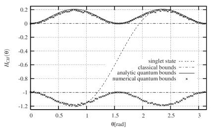
Figure 1: Numerical simulation of the bounds of the CHSH-inequality

The extension to three measurement operators for each particle merely yields one additional non-equivalent inequality (with respect to symmetries) collins-gisin03 ; sliwa03

$$I_{33}=p_{14}+p_{15}+p_{16}+p_{24}+p_{25}-p_{26}+p_{34}-p_{35}-p_{1}-2p_{4}-p_{5}\leq 0$$ (15)

among the 684 inequalities pitowsky01 representing the faces of the associated classical correlation polytope. The associated operator for symmetric measurement directions is given by

$$\begin{array}[]{lll}&O_{33}(0,\theta,2\theta,0,\theta,2\theta)=q_{14}(0,0)+q_{15}(0,\theta)+q_{16}(0,2\theta)+q_{24}(\theta,0)+q_{25}(\theta,\theta)-q_{26}(\theta,2\theta)+\\ &\quad+q_{34}(2\theta,\theta)-q_{35}(2\theta,\theta)-q_{1}(0)-2q_{4}(0)-q_{5}(\theta)\\ &\quad=\frac{1}{4}\left(\begin{array}[]{cccc}-4\sin^{2}\theta&0&0&0\\ 0&-5-2\cos\theta-3\cos 2\theta+2\cos 3\theta&4\cos^{2}\frac{\theta}{2}&2\sin\theta+3\sin 2\theta-2\sin 3\theta\\ 0&4\cos^{2}\frac{\theta}{2}&-2(3+\cos 2\theta)&-2\sin\theta\\ 0&2\sin\theta+3\sin 2\theta-2\sin 3\theta&-2\sin\theta&2\sin^{2}\frac{\theta}{2}\cos^{2}\frac{\theta}{2}(4\cos\theta-3)\end{array}\right),\end{array}$$ (16)

in the Bell basis $\{|\phi^{+}\rangle,|\psi^{+}\rangle,|\psi^{-}\rangle,|\phi^{-}\rangle\}\equiv\{(1,0,0,0)^{T},(0,1,0,0)^{T},(0,0,1,0)^{T},(0,0,0,1)^{T}\}$ with $|\psi^{\pm}\rangle=1/\sqrt{2}(|01\rangle\pm|10\rangle)$ and $|\phi^{\pm}\rangle=1/\sqrt{2}(|00\rangle\pm|11\rangle)$. In this basis, $O_{33}$ can be decomposed into a direct sum of a one-dimensional and a three-dimensional matrix $O_{33}=o_{1}\oplus o_{3}$, thus simplifying the calculations of the real eigenvalues. By using the Cardano method cocolicchio00 , these can be calculated to be

$$\lambda_{1} = -\sin^{2}\theta,$$

$$\lambda_{2} = -2\sqrt{|u|}\cos\frac{\xi}{3}-\frac{b}{3},$$

$$\lambda_{3,4} = \sqrt{|u(x)|}\Big{[}\cos\frac{\xi}{3}\pm\sin\frac{\xi}{3}\Big{]}-\frac{b}{3}.$$ (17)

Here, $u=1/9(3c-b^{2})$ and $\cos\xi=\frac{1}{54}\big{(}9bc-2b^{3}-27d\big{)}/\big{(}u\sqrt{|u|}\big{)}$ where $b=-\mbox{Tr}\,o_{3},\ c=1/2\Big{(}\mbox{Tr}\,^{2}o_{3}-\mbox{Tr}\,o_{3}^{2}\Big{)},\ d=-\det o_{3}$. (For convenience we have omitted the dependencies on $\theta$.) In Figure 2, the eigenvalues are plotted as functions of the parameter $\theta$.

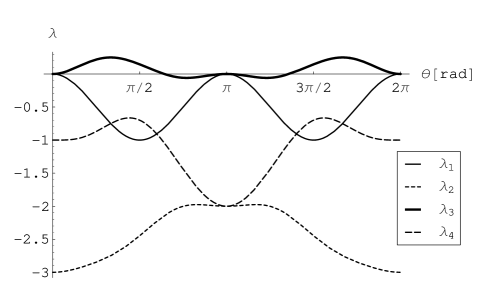
Figure 2: Eigenvalues of $O_{33}$ in dependence of the relative angle $\theta$.

The maximum violation of $1/4$ is obtained for $\theta=\pi/3$ with the eigenvector corresponding to $\lambda_{3}$

$$|\Psi_{\rm max}\rangle=\frac{\sqrt{3}}{2}|\phi^{-}\rangle+\frac{1}{2}|\psi^{+}\rangle.$$ (18)

$|\Psi_{\rm max}\rangle$ is maximally entangled, but in contrast to the CH-inequality, this is in general not the case for eigenstates corresponding to the maximal eigenvalue at $\theta\neq\pi/3$.

IV Relation to Experiments

The analytical quantum bound of the CH-operator has been enumerated by Cabello cabello04 as well as by the current authors filipp-svozil04a and experimentally verified by Bovino et al. bovino04 using polarization-entangled photon pairs. The ansatz of Cabello for the experimental realization made use of the fact that the eigenstates leading to maximal violations are maximally entangled. Thus when applying a unitary transformation $U(\theta)$ of the form

$$U(\theta)=\left(\begin{array}[]{cc}\sin\theta&-\cos\theta\\ \cos\theta&\sin\theta\end{array}\right)$$

onto an initial state $|{\psi^{-}}\rangle=\frac{1}{\sqrt{2}}(|{01}\rangle-|{10}\rangle)$, one obtains all maximally violating states for different $\theta$ values $|{\psi(\theta)}\rangle=U(\theta)\otimes 1_{2}|{\psi^{-}}\rangle$.

However, in the case of $O_{33}$, this scheme has to be extended, since the maximal violating states are not maximally entangled in general. Such states cannot be created from maximal entangled initial states by a local unitary operation $U_{2\times 2}\in SU(2)\otimes SU(2)$, since such a factorized transformation does not change the degree of entanglement. To obtain states constituting the quantum bounds, one has to apply unitary transformations $U_{4}\in SU(4)$ to the initial state comprising also non-local operations which cannot be written as a tensor product of two unitary single-particle operators.

A simplification for an experimental verification of the quantum bounds of Bell-type inequalities is due to the fact that maximal violating states are pure. Therefore, it is sufficient to generate initial states with variable degree of entanglement. Utilizing the Schmidt-decomposition, which is always possible for a bipartite state, one can write any pure state in the form $|{\psi}\rangle=\sum_{k}\lambda_{k}|{k_{1}}\rangle\otimes|{k_{2}}\rangle$ where $|{k_{j}}\rangle$ are orthonormal basis states for particle $1$ and $2$, respectively, and $\sum_{k}\lambda_{k}^{2}=1$. The weights of the $\lambda_{k}$’s are a measure of the degree of entanglement comprising the special cases where $\lambda_{1}=\lambda_{2}=1/\sqrt{2}$ for a maximally entangled state and $\lambda_{1}=0,\ \lambda_{2}=1$ (or vice versa) for a separable state. Having a source producing such states in a particular basis one can obtain all other pure states by applying a local unitary operation $U_{2\times 2}\in SU(2)\times SU(2)$. Appropriate photon sources have been suggested for example by White et al. White:1999 and Barbieri et al. barbieri04 and could therefore be used to trace the bounds on arbitrary bipartite Bell-type inequalities in the same manner as in the experiment of Bovino et al. bovino04 .

V Conclusion

In conclusion we have shown how to obtain analytically the quantum bounds on Bell-type inequalities for a particular choice of measurement operators. We have also presented a numerical simulation for obtaining these bounds for the CH-inequality. We have provided a quantitative analysis and derived the exact quantum bounds for bipartite inequalities involving two or three measurements per site. The generalization to an arbitrary number of measurement parameters is straightforward as the dimensionality of the eigenvalue problem remains constant. For more than two particles the dimension of the matrix associated with a Bell-type operator increases exponentially. However, one may conjecture that such matrices can be decomposed into a direct sum of lower dimensional matrices.

In the context of this conference we also believe that the analytic expressions of the quantum bounds could serve as consistency criteria of mathematical models proposed to show that a violation of Bell-type inequalities does not necessarily imply the absence of a possible local-realistic theory from the logical point of view. It is claimed that violations can be achieved without abandoning a local and realistic position assuming for example time-dependencies of the random parameters hess-philipp01a , or “chameleon” effects accardi01 . Still, any appropriate model has to be in accordance with quantum mechanics not only qualitatively, but also quantitatively, and hence should reproduce also the “fine structure” of the quantum bounds as discussed above.

Finally, although there is no theoretical evidence for a stronger-than-quantum violation whatsoever, its mere possibility justifies the sampling of the fine structure of the quantum bounds from the experimental as well as the theoretical point of view in order to understand and verify the restriction imposed by quantum theory.

VI Acknowledgments

S. F. acknowledges the support of the Austrian Science Foundation, Project Nr. 1514, and the support of Prof. H. Rauch rendering investigations in such theoretical aspects of quantum mechanics possible.

References

- (1) Peres, A., Quantum Theory: Concepts and Methods, Kluwer Academic Publishers, Dordrecht, 1993.
- (2) Bell, J. S., Physics, 1, 195 (1964).
- (3) Boole, G., The Laws Of Thought, Dover Publications Inc., New York (1958); originally published by Macmillan in 1854.
- (4) Boole, G., Philosophical Transactions of the Royal Society of London, 152, 225 (1862).
- (5) Bell, J. S., Rev. Mod. Phys., 38, 447 (1966).
- (6) Clauser, J. F., Horne, M. A., Shimony, A., and Holt, R. A., Phys. Rev. Lett., 23, 880 (1969).
- (7) Clauser, J. F., and Horne, M. A., Phys. Rev. D, 10, 526 (1974).
- (8) Werner, R., and Wolf, M., Phys. Rev. A, 64, 032112 (2001).
- (9) Zukowski, M., and Brukner, C., Phys. Rev. Lett., 88, 210401 (2002).
- (10) Aspect, A., Dalibard, J., and Roger, G., Phys. Rev. Lett., 49, 1804 (1982).
- (11) Weihs, G., Jennewein, T., Simon, C., Weinfurter, H., and Zeilinger, A., Phys. Rev. Lett., 81, 539 (1998).
- (12) Rowe, M. A., Kielpinski, D., Meyer, V., Sackett, C. A., Itano, W. M., Monroe, C., and Wineland, D. J., Nature, 409, 791 (2001).
- (13) Hasegawa, Y., Loidl, R., Badurek, G., Baron, M., and Rauch, H., Nature, 425, 45 (2003).
- (14) Bovino, F., Castagnoli, G., Degiovanni, I. P., and Castelletto, S., Phys. Rev. Lett., 92, 060404 (2004).
- (15) Filipp, S., and Svozil, K., Phys. Rev. A, 69, 032101 (2004).
- (16) Cabello, A., Phys. Rev. Lett., 92, 060403 (2004).
- (17) Froissart, M., Il Nuovo Cimento, 64 B, 241 (1981).
- (18) Pitowsky, I., Quantum Probability - Quantum Logic, Lecture Notes in Physics 321, Springer-Verlag, Berlin Heidelberg, 1989.
- (19) Pitowsky, I., e-print: quant-ph/0112068 (2001).
- (20) Pitowsky, I., Brit. J. Phil. Sci., 45, 95 (1994).
- (21) Tsirelson, B., Lett. Math. Phys., 4, 93 (1980).
- (22) Ziegler, G. M., Lectures on polytopes, Springer, New York, 1994.
- (23) Pitowsky, I., and Svozil, K., Phys. Rev. A, 64, 014102 (2001).
- (24) Filipp, S., and Svozil, K., e-print: quant-ph/0105083 (2001).
- (25) Pitowsky, I., Mathematical Programming, 50, 395 (1991).
- (26) Khalfin, L., and Tsirelson, B., Found. Phys., 22, 879 (1992).
- (27) Masanes, L., eprint: quant-ph/0309137 (2003).
- (28) Filipp, S., and Svozil, K., eprint: quant-ph/0403175 (2004).
- (29) Popescu, S., and Rohrlich, D., Phys. Lett. A, 166, 293 (1992).
- (30) Mermin, N. D., Ann. N. Y. Acad. Sci., 755, 616 (1995).
- (31) Krenn, G., and Svozil, K., Found. Phys., 28, 971 (1998).
- (32) Landau, L., Phys. Lett. A, 120, 54 (1987).
- (33) Halmos, P. R., Finite-dimensional vector spaces, Springer, New York, Heidelberg, Berlin, 1974.
- (34) Braunstein, S. L., Mann, A., and Revzen, M., Phys. Rev. Lett., 68, 3259 (1992).
- (35) Collins, D., and Gisin, N., eprint: quant-ph/0306129 (2003).
- (36) Sliwa, C., Phys. Lett. A, 317, 165 (2003).
- (37) Cocolicchio, D., and Viggiano, D., J. Phys. A, 33, 5669 (2000).
- (38) White, A. G., James, D., Eberhard, P., and Kwiat, P., Phys. Rev. Lett., 83, 3103 (1999).
- (39) Barbieri, M., Martini, F. D., Nepi, G. D., and Mataloni, P., Phys. Rev. Lett., 92, 177901 (2004).
- (40) Hess, K., and Philipp, W., Proc. Nat. Acad. Sc. USA, 98, 14224 (2001).
- (41) Accardi, L., Imafuku, K., and Regoli, M., eprint: quant-ph/0110086 (2001).