Dynamical Imperfections in quantum computers

Abstract

We study the effects of dynamical imperfections in quantum computers. By considering an explicit example, we identify different regimes ranging from the low-frequency case, where the imperfections can be considered as static but with renormalized parameters, to the high frequency fluctuations, where the effects of imperfections are completely wiped out. We generalize our results by proving a theorem on the dynamical evolution of a system in the presence of dynamical perturbations.

In any experimental implementation of a quantum information protocol nielsen one has to face the presence of errors. The coupling of the quantum computer to the surrounding environment is responsible for decoherence chuang95 which ultimately degrades the performances of quantum computation. The presence of static imperfections, although not leading to any decoherence, may be also detrimental for quantum computers. For instance, a small inaccuracy in the coupling constants, inducing as a consequence to errors in quantum gates, can be tolerated only up to a certain threshold georgeot00 . Moreover, the role of static imperfections depends on the regime, chaotic or not, of the system under consideration georgeot00 . The stability of a quantum computation in the presence of static imperfections has been already analyzed both in terms of fidelity miquel97 ; georgeot00 ; benenti01 and entanglement montangero03 .

A strict separation in “static” imperfections and “dynamical” noise may not be always satisfactory. Dynamical noise may be considered at the same level as static imperfections, if its evolution occurs on a scale much larger than the computational time. In Ref. benenti01 it was suggested that the effects of static imperfections can be more disruptive than noise for quantum computation. In this Letter, we intend to explore this problem in more details. The model we consider, in spite of its simplicity, enables one to grasp the interplay between the different time scales that appear in the problem. We consider each qubit coupled to a stochastic variable which changes in time with a fixed frequency. Below a given threshold (frequency), the errors can be considered as static, and thus can be corrected by using any of the known methods. The difference between the chaotic and the other dynamical regimes, found for static imperfections, holds also in the quasi-static case. We then generalize our results, by proving a theorem that states that, under general assumptions, in a perturbed system, unitary dynamical errors are averaged to zero in probability. Our results might be relevant in the context of the strategies that have been proposed during the last few years in order to suppress decoherence preskill .

Model - Following georgeot00 ; benenti01 , we model a quantum computer as a lattice of interacting spins (qubits). Due to the unavoidable presence of imperfections, the spacing between the up and down states (external field) and the couplings between the qubits (exchange interactions) are both random and fluctuate in time. We consider $n$ qubits on a two-dimensional lattice, described by the Hamiltonian

$$H(t)=\sum_{j=1}^{n}[\Delta_{0}+\delta_{j}(t)]\sigma_{z}^{(j)}+\sum_{\langle i,j\rangle}J_{ij}(t)\sigma_{x}^{(i)}\sigma_{x}^{(j)},$$ (1)

where the $\sigma^{(i)}_{\alpha}$’s ($\alpha=x,y,z$) are the Pauli matrices for qubit $i$ and the second sum runs over nearest-neighbor pairs. The energy spacing between the up and down states of a qubit is $\Delta_{0}+\delta_{i}(t)$, where the $\delta_{i}(t)$’s are uniformly distributed in the interval $[-\delta/2,\delta/2]$ and the $J_{ij}(t)$’s in the interval $[-J,J]$ (zero means and variances $\delta^{2}\sigma^{2}$ and $4J^{2}\sigma^{2}$, respectively, with $\sigma^{2}=1/12$). We model the dynamical noise by supposing that both $\delta_{i}(t)$ and $J_{ij}(t)$ change randomly after a time interval $\tau$. Within the time interval they are constant.

For $J=\delta=0$ the spectrum of the Hamiltonian is composed of $n+1$ degenerate levels, with interlevel spacing $2\Delta_{0}$, corresponding to the energy required to flip a single qubit. We study the case $\delta,J\ll\Delta_{0}$, in which the degeneracies are resolved and the spectrum is composed by $n+1$ bands. In this limit the coupling between different bands is very weak. We assume free boundary conditions and express all the energy in units of $\Delta_{0}$ (we choose $\hbar=1$).

In the following we analyze the behavior of the fidelity peres and error

$$F(t)\equiv|\langle\Psi|U(t)|\Psi\rangle|^{2}\ ,\quad E=-\ln F\ .$$ (2)

starting from an initial state $|\Psi\rangle$ which is an eigenstate of $\sigma_{z}^{(j)}$ ($j=1,\ldots,n$), $U(t)$ being the unitary evolution generated by (1). We concentrate on the central band of zero total magnetization which is characterized by the highest density of states and for which one expects that the effect of noise is most pronounced.

Results - The decay of the fidelity due to static imperfections is displayed in the inset of Fig. 1. The system (1) is characterized by two distinct dynamical regimes depending on the critical value $J_{c}\sim\delta/n$: the Fermi Golden Rule (FGR) ($J<J_{c}$) and the ergodic regime ($J>J_{c}$) georgeot00 ; montangero03 . The FGR is characterized by a Lorentzian local density of states with width $\Gamma^{\rm FGR}$. The ergodic regime is reached when all the levels inside the band participate to the dynamics; the local density of states coincides with the density of states and has a Gaussian shape with variance $\Gamma^{\rm erg}$.

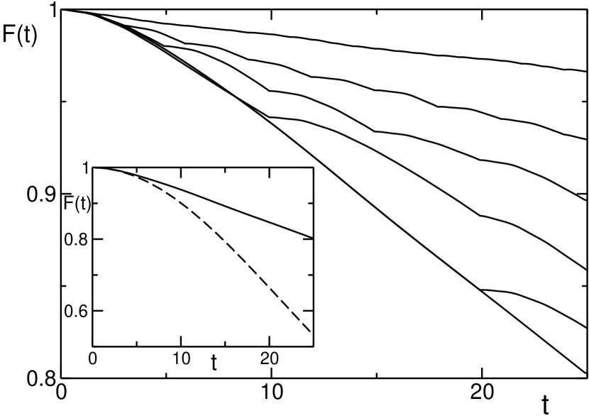
Figure 1: Fidelity as a function of time for $n=14$ qubits in the FGR regime ($J=2\cdot 10^{-2},\delta=4\cdot 10^{-1}$) and from top to bottom $\tau=1,3,5,10,20,25$ (static imperfections). Inset: Fidelity as a function of time in the ergodic ($J=\delta=2\cdot 10^{-2}$, dashed line), and in the FGR regime (full line).

In both regimes the decay of the fidelity is the Fourier transform of the local density of states flambaum and follows an exponential and a Gaussian decay with characteristic decay times $\Gamma_{\rm FGR}\propto J^{2}/\delta$ and $\Gamma_{\rm erg}\propto J^{2}$ respectively (see Inset Fig. 1) georgeot00 .

In the case of dynamical imperfections, different regimes emerge as a function of the frequency $1/\tau$. Below a critical timescale $\tau_{c}$ the different behavior due to the ergodic and FGR regimes cannot be resolved anymore. This can be clearly seen in Figs. 1-2. A smoother crossover appears at a higher frequency $1/\tau_{p}$ (Fig. 2) when the noise frequency become comparable with the single qubit natural frequency ($\sim\Delta_{0}$). The error $E_{t}(\tau)$ at (fixed) time $t$ tends to vanish as $\tau$ decreases.

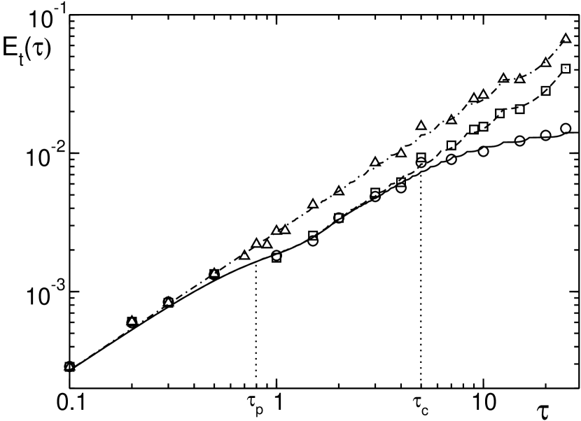
Figure 2: Error $E$ as a function of $\tau$ for $t=25,n=10,J=5\times 10^{-3}$, in the ergodic regime $\delta=5\times 10^{-3}$, $n_{\uparrow\downarrow}=8$ (squares), $n_{\uparrow\downarrow}=13$ (triangles) and in the FGR regime $\delta=3\times 10^{-1}$ (circles). The fits are given by Eqs. (3) and (5)-(6) with $\sigma^{2}=1/12$, $n_{c}=13$, $\Delta_{0}=1$ and $(n_{\uparrow\downarrow},n_{\uparrow\uparrow})$ equal to $(8,5)$ (dashed), $(13,0)$ (dot-dashed). The transition at $\tau_{c}$ is shown only in the former case. All the errors scale as $J^{2}$ (data not shown).

The explicit calculation of the error to order $J^{2}$ yields

$$E_{t}(\tau)=4J^{2}\sigma^{2}\left(Ng(\tau)+g(\Delta t)\right),$$ (3)

where $t=N\tau+\Delta t$, with $N$ integer, $0\leq\Delta t<\tau$, and

$$g(\tau)=2\int_{0}^{\tau}ds\int_{0}^{s}du\;\mathrm{sinc}^{2}\!(\delta u)\left[n_{\uparrow\downarrow}+n_{\uparrow\uparrow}\cos(4\Delta_{0}u)\right]\ ,$$ (4)

$n_{\uparrow\uparrow}$ ($n_{\uparrow\downarrow}$) being the number of nearest-neighbor parallel (antiparallel) pairs in the initial state and $\mathrm{sinc}(x)=\sin x/x$. The integration can be explicitly performed integration although the resulting analytic expression is not very transparent. Note that, due to the convexity of $g(\tau)$, the error $E_{t}(\tau)\leq 4J^{2}\sigma^{2}tg(\tau)/\tau$, being equal when $t/\tau=N$, thus providing a simple interpolation of (3). Moreover, the function $g(\tau)$ can be approximated in several important limits. For $\tau\delta\ll 1$, $\mathrm{sinc}^{2}\!(\delta u)\simeq 1$, whence

$$g(\tau)\simeq\tau^{2}\left[n_{\uparrow\downarrow}+n_{\uparrow\uparrow}\mathrm{sinc}^{2}\!(2\Delta_{0}\tau)\right]\ ,$$ (5)

which yields $g(\tau)\simeq n_{c}\tau^{2}$ for $\tau\lesssim\tau_{p}=\pi/4\Delta_{0}$ and $g(\tau)\simeq n_{\uparrow\downarrow}\tau^{2}$ (ergodic regime) for $\tau\gtrsim\tau_{p}$ (see Fig. 2), where the total number of links $n_{c}=n_{\uparrow\downarrow}+n_{\uparrow\uparrow}$, unlike $n_{\uparrow\downarrow}$ and $n_{\uparrow\uparrow}$, does not depend on the initial state $|\Psi\rangle$. On the other hand, when $\tau\delta\gg 1$, $\mathrm{sinc}^{2}\!(\delta u)\simeq\frac{\pi}{\delta}\delta(u)$ (FGR regime) and (4) reads

$$g(\tau)\simeq n_{\uparrow\downarrow}\frac{\pi}{\delta^{2}}\left[\delta\tau-\ln(2\delta\tau)-\gamma-1\right]\;,$$ (6)

where $\gamma\simeq 0.577$ is Euler’s constant. Substituting these approximate expressions in Eq. (3), the error at a fixed time $t$ for different $\tau$ values scales like

$$E_{t}(\tau)\simeq 4J^{2}\sigma^{2}t\left\{\begin{array}[]{lll}n_{c}\tau&\tau<\tau_{p}&\mbox{(all regimes)}\\ n_{\uparrow\downarrow}\tau&\tau_{p}<\tau<\tau_{c}&\mbox{(all regimes)}\\ n_{\uparrow\downarrow}\tau&\tau>\tau_{c},\;J\simeq\delta&\mbox{(ergodic)}\\ n_{\uparrow\downarrow}\pi/\delta&\tau>\tau_{c},\;J<\delta/n&\mbox{(FGR)}\end{array}\right.$$ (7)

In Fig. 2 we show the scaling of $E_{t}(\tau)$ with $\tau$ for different values of $J$. For the ergodic regime we choose $J=\delta$, while the FGR is characterized by $J\ll\delta$. As $\tau<\tau_{c}$ the two distinct ergodic and FGR behaviors of the static case (compared in Fig. 2 only for the sets with $n_{\uparrow\downarrow}=8$) are not resolved. Equations (5) and (6), plotted in Fig. 2, are in excellent agreement with the numerical results. The additional kink at $\tau\simeq\tau_{p}=\pi/4\Delta_{0}$ sets in when single spin dynamics starts to play a role. We also checked that $\tau_{p}$ is independent on $J$ and $\delta$, in agreement with Eq. (5). The transition at $\tau=\tau_{c}$ is striking and occurs when the error starts deviating from the linear behavior given by Eq. (7). In fact, the crossover between the two regimes could be defined by equating the third and the fourth line of (7), that is for $\tau=\pi/\delta$, which for $\delta=0.3$ would give $\tau\simeq 10.5$. However, since the saturation value $E_{t}(\tau)=4J^{2}\sigma^{2}n_{\uparrow\downarrow}\pi t/\delta$ given by Eq. (7) is reached only for $\delta\tau\gg 1$ and since the transition is sharp, a much more accurate way to define $\tau_{c}$ is by looking at the point for which the deviation from the linear behavior [third line in Eq. (7)] becomes apparent. To this purpose we keep the next-leading correction to Eq. (5) and approximate $\mathrm{sinc}^{2}\!(\delta u)\simeq 1-(\delta u)^{2}/3$ (for $\tau\lesssim 1/\delta$) in the integral (4). For $\tau\gtrsim\tau_{p}$ we obtain

$$g(\tau)\simeq\frac{n_{\uparrow\downarrow}}{\delta^{2}}\left[(\delta\tau)^{2}-\frac{(\delta\tau)^{4}}{18}\right]\,.$$ (8)

If the plot resolution in Fig. 2 is some fraction $\varepsilon$ of the total vertical range $4J^{2}\sigma^{2}n_{\uparrow\downarrow}t^{2}$, the error curve starts deviating from the linear behavior when $(t/\tau)(\delta\tau)^{4}/(18\delta^{2})\simeq\varepsilon t^{2}$, i.e.

$$\tau_{c}=\frac{(18\varepsilon t)^{\frac{1}{3}}}{\delta^{\frac{2}{3}}},$$ (9)

which for $t=25$, $\delta=0.3$ and $\varepsilon=1/40$ yields $\tau_{c}=5$, in full agreement with Fig. 2.

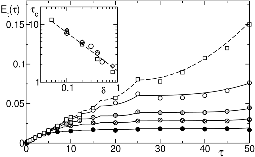
Figure 3: Error at time $t=50$, for $n=10,J=5\cdot 10^{-3}$ and different $\delta$ values. The squares represent the ergodic regime $\delta=J$. The FGR regime is plotted for $\delta=1,2,3,5\cdot 10^{-1}$ (empty, pointed, dashed, full circles respectively). Inset: $\tau_{c}$ as a function of $\delta$ for $n=10,12,14$ (circles, squares and diamonds respectively). The dashed line is proportional to $\delta^{-2/3}$, in agreement with Eq. (9).

In Fig. 3 we show the error $E_{t}(\tau)$ with fixed $J$ and different $\delta$ values. The scaling of the critical threshold $\tau_{c}$ is clearly visible. We also checked that $\tau_{c}$ does not depend on $J$ (data not shown). The inset of Fig. 3 shows the dependence of $\tau_{c}$ as a function of $\delta$, confirming the prediction (9).

Theorem - After having presented the overall picture of dynamical imperfections on the fidelity of computation, we complete our analysis and set up a general framework to consider the effect of a time-dependent noise on the evolution of a quantum system

$$H(t)=H_{0}+\xi(t)V,$$ (10)

where $H_{0}$ is time independent and $H(t)$ varies with a given characteristic time $\tau$, according to the stochastic process with independent increments $\xi(t)=\sum_{k=1}^{N}\chi_{[k\tau-\tau,k\tau)}(t)\;\xi_{k}$, where $\chi_{A}$ is the characteristic function of the set $A$ and $\{\xi_{k}\}_{k}$ are independent and identically distributed random variables, with expectations $E[\xi_{k}]=0,~{}\mathrm{Var}[\xi_{k}]=E[\xi_{k}^{2}]=\sigma^{2}<\infty.$ The time evolution operator over the total time $t=\tau N$ is given by

$$U_{N}(t)=\prod_{k=1}^{t/\tau}\exp[-i(H_{0}+\xi_{k}V)\tau],$$ (11)

where a time-ordered product is understood, with earlier times (lower $k$) at the right. Let us assume, for simplicity, that $H_{0}$ and $V$ are bounded operators, so that $U(t)$ is a norm-continuous one-parameter group of unitaries and all our subsequent estimates are valid in norm. We are interested in the existence and form of the limiting time evolution operator $U_{N}(t)$ for $N\to\infty$. When expanding the product, one finds that the term independent of $t$ is $1$, while the term proportional to $t$ reads $-iH_{0}t-iVt\sum_{k=1}^{N}\xi_{k}/N$. Now, according to the weak law of large numbers Cheb , $P\!-\!\lim_{N\to\infty}\sum_{k=1}^{N}\xi_{k}/N=E[\xi_{k}]=0$, for we assumed $E[\xi_{k}^{2}]=\sigma^{2}<\infty$, and the limit is taken in probability. Therefore, for $N\to\infty$

$$1-iH_{0}t-iVt\frac{1}{N}\sum_{k=1}^{N}\xi_{k}\stackrel{{\scriptstyle P}}{{\longrightarrow}}1-iH_{0}t.$$ (12)

Analogously, by using the weak law of large numbers, one can prove that all higher powers of $Vt$ vanish in the limit, thus obtaining

$$U(t)\equiv P\!-\!\!\!\lim_{N\to\infty}U_{N}(t)=\exp(-iH_{0}t),$$ (13)

in the following sense

$$\lim_{N\to\infty}P\left(\|U_{N}(t)-\exp(-iH_{0}t)\|\geq\varepsilon\right)=0,$$ (14)

uniformly in each compact time interval. If the term $\xi(t)V$ is viewed as exemplifying the effect of (dynamical) error-inducing disturbances, the above result physically implies that the effects of the errors are wiped out if their characteristic frequency $\tau^{-1}$ is sufficiently fast. This defines the purely dynamical regime.

Another viewpoint can also be adopted, that is somewhat complementary to the above one. Given a characteristic frequency of the noise, it is possible to establish an effective value of the strength of the imperfections so that the above result holds (approximately). In this sense, a natural question is what happens for large but finite $N$. This (physical) question can be answered by remembering that under the same hypotheses, according to the central limit theorem, the limiting random variable $\eta=\lim_{N\to\infty}\sum_{k=1}^{N}\xi_{k}/\sqrt{N}$ exists and is Gaussian with mean $E[\eta]=0$ and variance $E[\eta^{2}]=\sigma^{2}$, namely it is distributed like $f(\eta)=(2\pi\sigma^{2})^{-\frac{1}{2}}\exp(-\eta^{2}/2\sigma^{2})$. Thus, by following the same steps that led to (13) we find that for $N\gg 1$

$$U_{N}(t)\sim\exp\left[-i\left(H_{0}+\eta V/\sqrt{N}\right)t\right].$$ (15)

Equation (15) implies then that for fixed $\tau$, the system “feels” an effective interaction strength $\epsilon_{\rm eff}=\sigma\|V\|/\sqrt{N}\propto\sigma\|V\|\sqrt{\tau}$.

For intermediate values of $N$, Eq. (15) is no longer valid, because it hinges upon the commutativity of $H_{0}$ and $V$. However, by assuming that $V\ll H_{0}$ (e.g. in norm), a straightforward expansion shows that the perturbation $V$ is replaced by

$$\bar{V}(\tau)=\frac{1}{\tau}\int_{0}^{\tau}dt\;e^{iH_{0}t}Ve^{-iH_{0}t}\ ,$$ (16)

so that, for $\tau\|H_{0}\|\gtrsim 2\pi$, the effective perturbation becomes

$$\bar{V}(\tau)\to V_{Z}=\sum_{k}P_{k}VP_{k},$$ (17)

where $P_{k}$ are the eigenprojections of $H_{0}$ ($H_{0}=\sum\lambda_{k}P_{k}$). This phenomenon is reminiscent of the quantum Zeno subspaces theorem .

The generalization of the above results to a Hamiltonian with a family of independent stochastic processes with zero mean and finite variances is straightforward. This is the case of the Hamiltonian (1), which reads

$$H(t)=H_{0}+\delta\;\bm{\xi_{0}}(t)\cdot\bm{V_{0}}+2J\;\bm{\xi}(t)\cdot\bm{V},$$ (18)

where $H_{0}=\sum_{j}\Delta_{0}\sigma_{z}^{(j)}$, $(\bm{V}_{0})_{j}=\sigma_{z}^{(j)}$, $(\bm{V})_{ij}=\sigma_{x}^{(i)}\sigma_{x}^{(j)}$, and $\xi_{0j}=(\bm{\xi}_{0})_{j}$ and $\xi_{ij}=(\bm{\xi})_{ij}$ $(i,j=1,\cdots,n)$ are independent random variables uniformly distributed in the interval $[-1/2,1/2]$.

We can then reinterpret our previous results in the light of the above theorem, by applying the well-known static results flambaum to the (static) evolution with renormalized couplings (15) (with $\eta V\rightarrow\bm{\eta}\cdot\bm{V}$). Thus, independently of the interaction strength and the correspondent dynamical regime, there is a quadratic decay law for sufficiently large $N=t/\tau$ (or small $\tau$),

$$E_{t}(\tau)\sim\frac{1}{N}\frac{t^{2}}{\tau_{Z}^{2}}=\frac{t}{\tau_{Z}^{2}}\tau\quad(\tau<\tau_{p}),$$ (19)

where $\tau_{Z}^{-2}=4J^{2}\langle\Psi|(\bm{\eta}\cdot\bm{V})^{2}|\Psi\rangle=4J^{2}n_{c}\sigma^{2}$ and $\tau_{p}\simeq\Delta_{0}^{-1}$ [the $H_{0}$-timescale, see (16)]. On the other hand, for smaller $N$, i.e. $\tau>\tau_{p}$, the effective interaction (17) is given by $(\bm{V}_{Z})_{ij}=\sigma_{+}^{(i)}\sigma_{-}^{(j)}+\sigma_{-}^{(i)}\sigma_{+}^{(j)}$, whence

$$E_{t}(\tau)\sim\frac{1}{N}\Gamma_{\mathrm{erg}}t^{2}=\Gamma_{\mathrm{erg}}t\tau\quad(\tau>\tau_{p}),$$ (20)

where $\Gamma_{\mathrm{erg}}=4J^{2}\langle\Psi|(\bm{\eta}\cdot\bm{V}_{Z})^{2}|\Psi\rangle=4J^{2}n_{\uparrow\downarrow}\sigma^{2}$. Therefore, we recover the linear growth of the error (with the correct coefficients), that describes both regimes up to $\tau_{c}$ in Eq. (7).

Conclusions - We studied the effects of dynamical imperfections on a general model of a quantum computer and identified several dynamical regimes, depending on the frequency of the external noise as compared with the coupling constants of the quantum computer. Above a threshold frequency, imperfections can be treated as static imperfections, although with renormalized parameters. Below this threshold the different dynamical regimes induced by the presence of imperfections are not resolved. These results give a better comprehension of the general problem of noise in quantum computers and might suggest new strategies to develop general error correcting techniques.

This work was supported by the European Community under contracts IST-SQUIBIT, IST-SQUBIT2 and RTN-Nanoscale Dynamics.

References

(1)
M.A. Nielsen and I.L. Chuang, Quantum
computation and quantum information, (Cambridge Univ. Press,
2000).
(2)
I.L. Chuang, R. Laflamme, P.W. Shor and W.H. Zurek, Science,
270, 1635 (1995)
(3)
B. Georgeot and D.L. Shepelyansky, Phys. Rev. E 62,
3504 (2000); 62, 6366 (2000).
(4)
G. Benenti, G. Casati, S. Montangero,
D.L. Shepelyansky, Phys. Rev. Lett. 87, 227901 (2001).
(5)
C. Miquel, J.P. Paz, W.H. Zurek,
Phys. Rev. Lett. 78, 3971 (1997).
(6)
S. Montangero, G. Benenti, and R. Fazio,
Phys. Rev. Lett. 91, 187901 (2003).
(7)
A. Ekert, C. Macchiavello, Acta Phys.Polon. A93 63 (1998).
quant-ph/9904070.
(8)
A. Peres, Phys. Rev. A 30 1610 (1984).
(9)
V.V. Flambaum, Aust. J. Phys. 53, N4, (2000).
(10)
, where
and ; ,
and
being the cosine and sine integral functions and Euler’s
constant, respectively.
(11)
W. Feller, Probability Theory and its Applications,
vol. II (John Wiley, 1971)
(12)
P. Facchi and S. Pascazio, Phys. Rev. Lett. 89 080401 (2002)