Thermal entanglement of spins in an inhomogeneous magnetic field
M. Asoudeh,       V. Karimipour

Department of Physics, Sharif University of Technology,

P.O. Box 11365-9161,

Tehran, Iran

We study the effect of inhomogeneities in the magnetic field on the thermal entanglement of a two spin system. We show that in the ferromagnetic case a very small inhomogeneity is capable to produce large values of thermal entanglement. This shows that the absence of entanglement in the ferromagnetic Heisenberg system is highly unstable against inhomogeneoity of magnetic fields which is inevitably present in any solid state realization of qubits.

1 Introduction

1.1 Motivation

It is well known that quantum entanglement [1, 2, 3] plays a fundamental role in almost all efficient protocols of quantum computation (QC) and quantum information processing [4, 5].
Without entanglement which is the essential quantum ingredient of QC, any quantum algorithm which only uses the other property of quantum mechanics, namely the superposition property, can also be implemented on any physical system which allows superposition of states, i.e. classical linear optical devices. In any proposal for physical implementation of qubits, it is therefore of utmost importance to investigate the entanglement properties of pairs and collection of such qubits. Among the many proposals for physical implementation of qubits, those based on solid state devices seem to be promising as far as the crucial scalablity property is concerned.
In one such proposal [6] a well localized nuclear spin coupled with an electron of a donor atom in silicon plays the role of a qubit which can be individually initialized, manipulated and read out by extremely sensitive devices. In another proposal[7, 8, 9, 10], the spin of an electron in a quantum dot plays the role of a qubit. Long decoherence time and scalability to more than 100 qubits are two of the important virtues of this scheme.
In both schemes the effective interaction between the two qubits is governed by an isotropic Heisenberg Hamiltonian with Zeeman coupling of the individual spins, namely

$$H=J{\bf S}_{1}\cdot{\bf S}_{2}+\gamma(S_{1z}+S_{2z}).$$ (1)

Actually the isptropic interaction is an approximation, since spin orbit coupling introduce perturbations which break this isotropy . A more complete hamiltonian would be [11, 12]

$$H=J({\bf S}_{1}\cdot{\bf S}_{2}+\overrightarrow{\beta}\cdot{\bf S}_{1}\times{\bf S}_{2}+\gamma\overrightarrow{\beta}\cdot{\bf S}_{1}\overrightarrow{\beta}\cdot{\bf S}_{2})+\gamma(S_{1z}+S_{2z}),$$ (2)

where the dimensionless vector $\overrightarrow{\beta}$ is called the spin orbit field and in systems like the GaAs quantum dots has a magnitude $|\overrightarrow{\beta}|$ of a few percent and the dimensionless $\gamma$ is of the order of $10^{-4}$. Note that the only coupling in the interaction between spins that is controllable is $J$ [12], and the individual couplings between different components of spins denoted usually by $J_{x},J_{y}$ and $J_{z}$ can not be controlled separately and thus one can not adjust these parameters arbitrarily to enhance the entanglement in a given situation.
This means that although studies of entanglement for different types of anisotropic interactions are very interesting theoretically (specially when infinite spin systems are treated which is the only case which yields valid results with regard to quantum phase transitions [13]), they may not be of much practical relevance to concrete physical realization of qubits.
In this paper we ignore the anisotropic perturbations due to both their smallness and due to the fact that strategies have been invented to cancel such anisotropies [14].
Due to their smallness, they may only introduce minor changes in any result derived for the isotropic case.
On the other hand in any solid state construction of qubits, there is always the possibility of inhomogenous Zeeman coupling [15, 16]. Solid state heterostructures are usually inhomogeneous and magnetic imperfections or impurities are likely to be present leading to stray magnetic fields. Indeed it is one of the main challenges in this proposal to construct identical qubits [17]. Constructing nearly identical devices in semiconductor technology has always been difficult and is still difficult, e.g. a very small temperature or strain difference in the substrate produces differences which although may not be significant for the classical semiconductor technology will certainly be important for the quantum technology [17]. Besides these unwanted effects, there are schemes like parallel pulsed schemes [18], in which both a localized and hence inhomogenous Zeeman coupling and exchange interactions are employed to expedite manipulation of qubits.

In view of the above it is desirable to consider a two qubit system in an inhomogenous magnetic field and study the entanglement properties of this system in detail.
At extremely low temperatures such a qubit system may be assumed to be in its ground state. Thus it will be desirable to study the entanglement properties of the ground state.
However a real physical system is always at a finite temperature and hence in a mixture of disentangled and entangled states depending on the temperature. Therefore one is naturally led to consider the thermal entanglement of such physical systems.
In summary we mean that the thermal entanglement of finite systems has more relevance to the problem of initialization of quantum computers [19] than to the problem of quantum phase transitions which requires a study of infinite size systems.

1.2 A brief account of previous works

Thermal entanglement in a two qubit Heisenberg magnet with the Hamiltonian

$$H=J\overrightarrow{\sigma}_{1}\cdot\overrightarrow{\sigma}_{2}+B(\sigma_{1z}+\sigma_{2z}).$$ (3)

was first studied by Nielsen [21] who showed that in the ferromagnetic case ($J<0$) no entanglement exists but in the antiferromagnetic case ($J>0$) entanglement appears below a threshold temperature $T_{c}$. Since then many other systems have been investigated.
There is now a vast literature on this subject and for clarity it is better to separate them into two categories, namely those [22, 23, 24, 25, 26] which study by analytical or numerical methods infinite spin chains with at times particular attention to quantum phase transitions and those which study few, mostly two, spin systems. In our opinion one can not draw valid results for quantum phase transitions by studying a two spin system, and these types of studies are useful in other contexts, e.g. the problem of initialization of a quantum computer as described above, provided they start with a plausible hamiltonian for the interaction of physical qubits.
In the following we mention some of the works only in this latter category which are of relevance to our work in this paper.
After the work of Nielson [21], it has been shown that two spins interacting by the Ising interaction in the $z$ direction, when placed in a magnetic field of arbitrary direction, acquire maximum entanglement when the magnetic field is perpendicular to the $z$ direction [27].
The effect of anisotropy (in the spin couplings in the $x$, $y$ and $z$ directions) has also been studied in a number of works for different models [28, 29, 30, 31]. The effect of inhomogeneous magnetic fields has been studied in [32], but only on an $XY$ system. Such a system already shows entanglement when placed in a uniform magnetic field.

1.3 Results

In this paper we have studied an isotropic two qubit system in a inhomogeneous magnetic field, described by the Hamiltonian

$$H=J\overrightarrow{\sigma}_{1}\cdot\overrightarrow{\sigma}_{2}+(B+b)\sigma_{1z}+(B-b)\sigma_{2z},$$ (4)

where $J$ is the isotropic coupling between the spins, $B\geq 0$, and the magnetic fields on the two spins have been so parameterized that $b$ controls the degree of inhomogeneity.

Let us first review the situation for the homogeneous magnetic field.

For the ferromagnetic ($J<0$) system, there is no thermal entanglement at any temperature, but for the anti-ferromagnetic ($J>0$) case, thermal entanglement develops when the temperature drops below the threshold value $kT_{c}:=\frac{4J}{\ln 3}$. We want to see how the presence of inhomogeneity modifies this situation. We will show that inhomogeneity has the following effects:

1- In the ferromagnetic system it generally produces entanglement, dependent on the value of the magnetic field and the temperature. There is a threshold temperature above which no entanglement is possible. This temperature has in fact been zero in the uniform case which has been shifted to finite values by the inhomogeneity. Specially at temperatures near zero and in zero magnetic field, the effect of inhomogeneity is very significant. Under this condition a very small inhomogeneity produces maximal entanglement as shown in figures (3 and 4).

2- In contrast to the ferromagnetic case, the effects in the anti-ferromagnetic system are small. Inhomogeneity in this case slightly raises the threshold temperature, and lowers the value of entanglement as shown in figures (5 and 6).

The structure of this paper is as follows: After presenting the essentials of thermal entanglement in the next section, in section 3 we study the spectrum of the Hamiltonian and characterize the entanglement of the ground state in various regions of the parameter space. In section 4 we analyze the thermal entanglement of the system. Throughout the paper we normalize the coupling between spins to $J=1$ for the anti-ferromagnetic case and to $J=-1$ for the ferromagnetic case and study the results for the two cases separately.

2 Preliminaries on thermal entanglement

A spin system with Hamiltonian $H$ kept at temperature $T$ is characterized by a density matrix $\rho:=\frac{1}{Z}e^{-\beta H}$, where $\beta=\frac{1}{kT}$, $k$ is the Boltzman constant and $Z:=tre^{-\beta H}$ is the partition function.
The entanglement of this density matrix, called the thermal entanglement of the spin system can be calculated exactly with the help of Wootters formula [20]. Explicitly it is given by the following formula

$$E(\rho)=-\frac{1+\sqrt{1-C^{2}}}{2}\log_{2}{\frac{1+\sqrt{1-C^{2}}}{2}}-\frac{1-\sqrt{1-C^{2}}}{2}\log_{2}{\frac{1-\sqrt{1-C^{2}}}{2}},$$ (5)

where

$$C=max\{0,\lambda_{1}-\lambda_{2}-\lambda_{3}-\lambda_{4}\},$$ (6)

and $\lambda$’s are the positive square roots of the eigenvalues of the matrix $\rho\tilde{\rho}$ in decreasing order. The matrix $\tilde{\rho}$ is defined as

$$\tilde{\rho}=(\sigma^{y}\otimes\sigma^{y})\rho^{*}(\sigma^{y}\otimes\sigma^{y}),$$ (7)

where $*$ denotes complex conjugation in the computational basis.
In case that the state is pure $\rho=|\psi\rangle\langle\psi|$, with

$$|\psi\rangle:=a|+,+\rangle+b|+,-\rangle+c|-,+\rangle+d|-,-\rangle$$ (8)

the above formula for the concurrence is simplified to

$$C(\psi)=2|ad-bc|.$$ (9)

Since $E$ is an increasing function of $C$, it is usual to take $C$ itself as a measure of entanglement whose value ranges from $0$ for a disentangled state to $1$ for a maximally entangled state. In the following sections we apply this formalism to the inhomogeneous system given by the Hamiltonian (4).

3 Ground state entanglement

When the magnetic field is uniform, i.e. $b=0$, the hamiltonian (4) has two symmetries, namely $[H,S_{z}]=[H,S^{2}]=0$, where $S_{z}$ and $S^{2}$ are the third component of spin and the total spin respectively. In a inhomogeneous magnetic field, the symmetry $[H,S^{2}]=0$ no longer holds and thus the triplet and the singlet spins are no longer energy eigenstates separately. A straightforward calculation gives the following eigenstates:

$$|\phi_{1}\rangle = |+,+\rangle$$ (10)

$$|\phi_{2}\rangle = |-,-\rangle$$ (11)

$$|\phi_{3}\rangle = \frac{1}{\sqrt{2({\delta}^{2}+(1-\xi)^{2})}}\left((\delta-1+\xi)|+,-\rangle+(\delta+1-\xi)|-,+\rangle\right)$$ (12)

$$|\phi_{4}\rangle = \frac{1}{\sqrt{2({\delta}^{2}+(1-\xi)^{2})}}\left((\delta+1-\xi)|+,-\rangle-(\delta-1+\xi)|-,+\rangle\right),$$ (13)

with corresponding energies

$$E_{1} = J+2B$$ (14)

$$E_{2} = J-2B$$ (15)

$$E_{3} = -J(1-2\xi)$$ (16)

$$\ E_{4} = -J(1+2\xi),$$ (17)

where $\xi:=\sqrt{1+\delta^{2}}$ and $\delta=\frac{b}{J}$.
Note that we are working in units so that $B$ and $J$ are dimensionless. It turns out that $\xi$ is the suitable parameter for expressing the effects of inhomogeneity. Thus hereafter we will mostly use $\xi$ rather than the original parameter $b$, in our analysis. The value $\xi=1$ corresponds to a uniform magnetic field and deviations from this value characterize the degree of non-uniformity.
In the limiting case $\xi\longrightarrow 1$, the two states $|\phi_{1}\rangle$ and $|\phi_{2}\rangle$ respectively go to the maximally entangled states $\frac{1}{\sqrt{2}}(|+,-\rangle+|-,+\rangle)$ and $\frac{1}{\sqrt{2}}(|+,-\rangle-|-,+\rangle)$.

3.1 The ferromagnetic case, $\ J=-1$

The ground state depends on the value of the magnetic field $B$ and the inhomogeneity parameter $\xi$. It is readily found that the ground state energy is equal to:

$$\left\{\begin{array}[]{l}E_{2}=-1-2B\ \ \ \ \ {if\ \ \ \ \ \xi<B+1},\\ \\ E_{3}=\ 1-2\xi\ \ \ \ \ \ {if\ \ \ \ \ \xi>B+1}\end{array}\right.$$ (21)

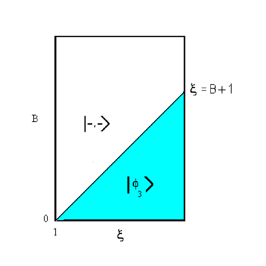
Figure 1: (color online)The ground state of the ferromagnetic case, as a function of inhomogeneity $\xi$ and the magnetic field $B$. We work in units where $B$ is dimensionless.

Thus for $\xi<B+1$, the ground state is the disentangled state $|\phi_{2}\rangle$ and for $\xi>B+1$, the ground state is the entangled state $|\phi_{3}\rangle$.
The phase diagram of the ground state is shown in figure (1).
For each value of the magnetic field $B$, there is a threshold parameter $\xi^{f}:=B+1$ above which the ground state will become entangled. Conversely for each value of inhomogeneity $\xi$ there is a value of magnetic field $B^{f}:=\xi-1$ above which the ground state will loose its entanglement.
In the entangled phase the entanglemenet of the ground state is found from (9) and (10) to be

$$C(\phi_{3})=\frac{1}{\xi},$$ (22)

which is solely determined by inhomogeneity. A very interesting point is that when $B=0$, with an infinitesimal value of $b\approx 0$ ($\xi\approx 1$) the system enters the maximally entangled phase $|\phi_{3}\rangle$ with etanglment $C=\frac{1}{\xi}\approx 1$. This remarkable feature means that the absence of entanglement in ferromagnetic Heisenberg chain is completely unstable against very small inhomogeneities. It is also reminiscent of quantum phase transitions where a slight change in one of the parameters of the system, changes the behavior of the system dramatically. Increasing further the inhomogeneity will move the ground state further into the entangled phase but reduces its entanglement due to (22).

3.2 The anti-ferromagnetic case, $\ J=1$

In this case we find that the ground state energy is equal to

$$\left\{\begin{array}[]{l}E_{2}=1-2B\ \ \ \ \ \ {if\ \ \ \ \xi<B-1},\\ \\ E_{4}=\ -1-2\xi\ \ \ \ \ \ {if\ \ \ \ \xi>B-1}\end{array}\right.$$ (26)

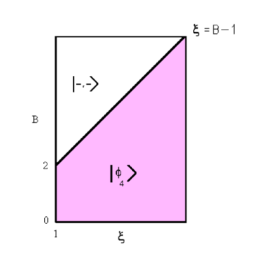
Figure 2: (color online) The ground state of the antiferrmagnetic case, as a function of inhomogeneity $\xi$ and the magnetic field $B$. We work in units where $B$ is dimensionless.

Thus for $\xi<B-1$, the ground state is the disentangled state $|\phi_{2}\rangle$ and for $\xi>B-1$, the ground state is the entangled state $|\phi_{4}\rangle$. The phase diagram of the ground state is shown in figure (2).

Again in the entangled phase the entanglement of the ground state is found from (9) and (10) to be

$$C(\phi_{4})=\frac{1}{\xi}.$$ (27)

which is independent of $B$. Increasing inhomogeneity again decreases the concurrence and hence the entanglement.

4 Thermal entanglement

Raising the temperature mixes the ground state with excited states. Depending on the sign of $J$ and the value of parameters this may increase or decrease the value of entanglement. In some cases the disentangled ground state mixes with entangled excited states and in some other cases the entangled ground state mixes with disentangled excited states. To see what happens exactly we calculate the entanglement of the thermal state $\rho=\frac{1}{Z}e^{-\beta H}$. The symmetry $[H,S_{z}]=0$ constrains the general form of $\rho$ to

$$\rho=\left(\begin{array}[]{cccc}u_{+}&&&\\ &w&z&\\ &z&w&\\ &&&u^{-}\\ \end{array}\right),$$ (28)

where $C$ is found from (6 and 7) to be given [22] by

$$C=2\ {\rm{max}}\ (0,|z|-\sqrt{u^{+}u^{-}}).$$ (29)

The exact values of the elements of $\rho$ is obtained by knowing the spectrum of $H$. After a simple calculation from

$$\rho=\frac{1}{Z}\sum_{i=1}^{4}e^{-\beta E_{i}}|\phi_{i}\rangle\langle\phi_{i}|$$ (30)

we obtain

$$u_{+} = \frac{1}{Z}e^{-\beta(J+2B)},$$ (31)

$$u_{-} = \frac{1}{Z}e^{-\beta(J-2B)},$$ (32)

and

$$z=\frac{-1}{Z}\frac{1}{\xi}e^{\beta J}\sinh{2J\beta\xi},$$ (33)

where $Z$ is the partition function given by

$$Z:=tre^{-\beta H}=2e^{-\beta J}\cosh{2\beta B}+2e^{\beta J}\cosh{2\beta J\xi}.$$ (34)

Thus from (29) we find that

$$C=\frac{2}{Z}\ \ {\rm{Max}}\ \left(0\ ,\ \frac{1}{\xi}e^{\beta J}|\sinh{2\beta J\xi}|-e^{-\beta J}\right).$$ (35)

We consider the ferromagnetic ($J=-1$) and the anti-ferromagnetic ($J=1$) cases separately.

4.1 Ferromagnetic case, $J=-1$

Setting $J=-1$ in (35) we have

$$C={\rm{Max}}\ \left(0,\frac{e^{-\beta}\sinh{2\beta\xi}-\xi e^{\beta}}{\xi(e^{\beta}\cosh{2\beta B}+e^{-\beta}\cosh{2\beta\xi})}\right).$$ (36)

The threshold temperature is obtained from the equation

$$e^{-2\beta}\sinh{2\beta\xi}=\xi.$$ (37)

In the uniform case ($\xi=1$), this equation turns into $e^{4\beta}=-1$ which has no solution. Thus in this limit there is no thermal entanglement in the spin system in accordance with previous results ([21, 23, 24]).
However in the inhomogeneous case ($\xi\neq 1$) this equation has nontrivial solutions. Figure (7) shows the variation of threshold temperature with $\xi$.

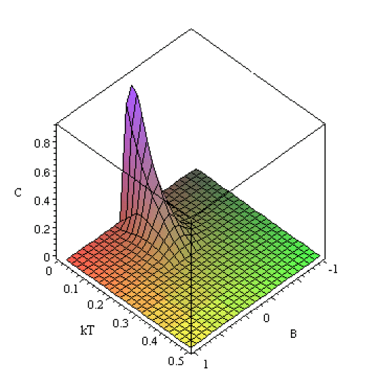
Figure 3: (color online) Concurrence versus temperature and magnetic field for $\xi=1.1$ in the ferromagnetic system.

Figure (3) shows the entanglement as measured by the concurrence for a fixed value of inhomogeneity $\xi=1.1$ in terms of the temperature and magnetic field. Below the threshold temperature (about $0.25$ for this value of $\xi$), thermal entanglement develops and is maximized for zero magnetic field $B$. The value of this maximum entanglement occurs of course at $T=0$, where its value is equal to $\frac{1}{\xi}$, equal to 0.9 in this case.

Figure (4) shows the value of entanglement in terms of the temperature and the inhomogeneity for zero magnetic field.

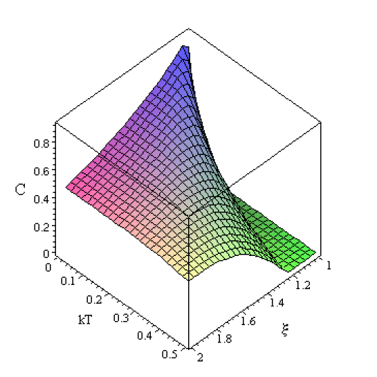
Figure 4: (color online) Concurrence versus temperature and inhomogeneity in zero magnetic field in the ferromagnetic system.

It is seen that at any temperature there is a parameter $\xi_{0}$ above which thermal entanglement will develop in the system. The value of $\xi_{0}$ is obtained from (37) and increases with increasing the temperature. At very low temperatures $\xi_{0}$ is very close to $1$ which shows that a small degree of inhomogeneity will develop maximal entanglement in the system.

4.2 Anti-Ferromagnetic case

Setting $J=1$ in (35) we obtain

$$C={\rm{Max}}\ \left(0,\frac{e^{\beta}\sinh{2\beta\xi}-\xi e^{-\beta}}{\xi(e^{-\beta}\cosh{2\beta B}+e^{\beta}\cosh{2\beta\xi})}\right)$$ (38)

The threshold temperature is obtained from the equation

$$e^{2\beta}\sinh{2\beta\xi}=\xi.$$ (39)

In the uniform case ($\xi=1$), this equation turns into $e^{4\beta}=3$ which gives the threshold temperature $kT_{c}=\frac{4}{\ln 3}$ .
In the inhomogeneous case ($\xi\geq 1$) this equation can be solved numerically, the results is shown in figure (7). It is seen that inhomogeneity only slightly increases the threshold temperature in contrast to the ferromagnetic case where it had appreciable effect.
Figure (5) shows the entanglement as measured by the concurrence for a fixed value of inhomogeneity $\xi=1.1$ in terms of the temperature and the magnetic field and figure (6) shows the value of entanglement in terms of the temperature and the inhomogeneity for zero magnetic field. Comparing these figures with figure (3) and with the corresponding figure of ([23]) we see that in the anti-ferromagnetic case, inhomogeneity has a small effect on the threshold temperature and magnetic field and only decreases the value of entanglement once it is developed. Its value is weakened by raising the temperature and near the threshold temperature it has a vanishingly small effect.

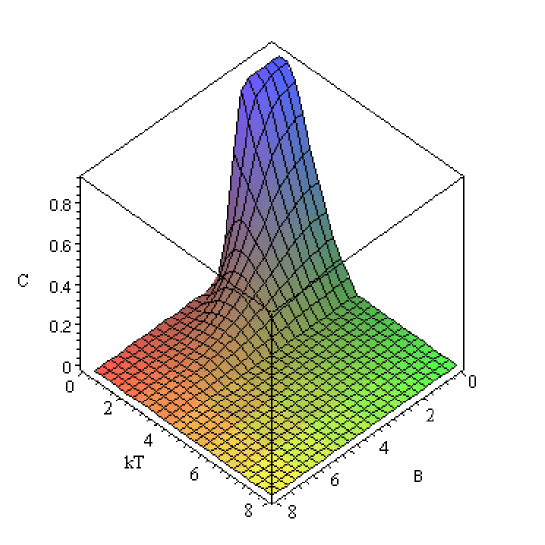
Figure 5: (color online) Concurrence versus temperature and magnetic field for $\xi=1.1$ in the anti-ferromgnetic system.

It is seen that for any fixed temperature inhomogeneity always decreases entanglement, in contrast to the ferromagnetic case.

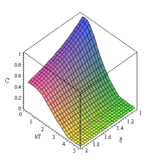
Figure 6: (color online) Concurrence versus temperature and inhomogeneity in zero magnetic field in the anti-ferromagnetic system.

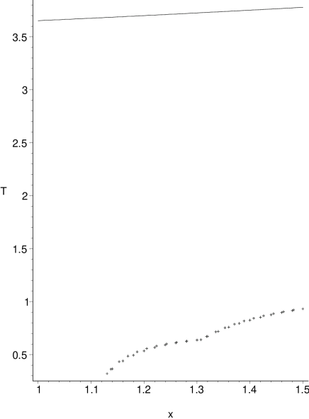
Figure 7: The variation of threshold temperature with inhomogeneity (denoted here as x) of the magnetic field in the ferromagnetic (dotted line) and anti-ferromagnetic (solid line) cases.

5 Discussion

We have studied the effect of a inhomogeneous magnetic field on the ground state entanglement and thermal entanglement of a two spin system. We have shown that the effect of inhomogeneity is most pronounced on ferromagnetic spins, i.e. spins coupled by ferromagnetic interactions. At zero temperature an infinitesimal magnetic field applied to the two spins in opposite directions maximally entangles the two spins. It is as if we twist the two spins into an entangled state. This effect also exists at higher temperatures but to much less degree. When the coupling of the spins is anti-ferromagnetic inhomogeneity can only have a weakening effect on entanglement. Although we have derived our results by studying a two spin systems, these results may also hold true more or less on spin chains. A parameter like $\xi:=\sqrt{1+\langle b^{2}\rangle}$, where $\langle b^{2}\rangle$ is the average of inhomogeneity on all sites, i.e. $\langle b^{2}\rangle:=\frac{1}{N}\sum_{i=1}^{N}(B_{i}-\langle B\rangle)^{2}$, may characterize the influence of inhomogeneity on the entanglement of a spin chain.

References

- [1] A. Einstein, B. Podolsky and N. Rozen, Phys. Rev., 47, 777 (1935).
- [2] E. Schrodinger, Naturwissenschaften, 23, 807 (1935).
- [3] J. S. Bell, Physics 1, 195 (1964).
- [4] C. H. Bennett, and D. P. Divincenzo, Nature, bf 407, 247 (2000).
- [5] M. A. Nielson and I. L. Chuang, Quantum Computation and Quantum Information, (Cambrdige University Press, Cambrdige, 2000).
- [6] B. E. Kane, Nature, 393 133 (1998).
- [7] D. Loss and D. P. DiVincenzo, Phys. Rev. A 57, 120(1998); J. Levy, Phys. Rev. A 64, 052306 (2001).
- [8] DiVincenzo et al, NATURE, Vol. 408, p. 339-342 (2000).
- [9] G. Burkard and G. Loss, Phys. Rev. Lett. 88, 047903 (2002).
- [10] A. Imamoglu et al, Phys. Rev. Lett. 83, 4204 (1999).
- [11] K. V. Kavokin, Phys. Rev. B 64, 075305 (2001).
- [12] L. A. Wu and D. A. Lidar, Phys. Rev. A 66, 062314 (2002).
- [13] S. Sachdev, Quantum Phase Transitions, (Cambrdige University Press, Cambrdige, 1999.)
- [14] N. E. Bonesteel, D. Stepanenko, and D. P. DiVincenzo, Phys. Rev. Lett. 87, 207901 (2001).
- [15] X. Hu, and S. Das Sarma, Phys. Rev. A. 61, 062301(2000).
- [16] X. Hu, R. de Sousa and S. Das Sarma, Phys. Rev. Lett. 86, 918(2001).
- [17] R. W. Keyes, Physics World Digest, August 2002, p. 15.
- [18] G. Burkard et al, Phys. Rev. B 60, 11404 (1999).
- [19] D. P. DiVincenzo, The Physical Implementation of Quantum Computation, quant-ph/0002077.
- [20] S. Hill and W. K. Wootters, Phys. Rev. Lett. 78, 5022 (1997); W. K. Wootters, Phys. Rev. Letts. 80, 2245 (1998).
- [21] M. A. Nielson, PhD thesis, University of New Mexico(1998), quant-ph/0011036.
- [22] M. K. O’Conner and W. K. Wootters,Phys. Rev. A 63, 052302 (2001).
- [23] M. C. Arnesen, S. Bose, and V. Vedral, Phys. Rev. Lett. 87, 277901 (2001).
- [24] X. Wang, and P. Zanardi, Phys. Lett. A 301 (1-2), 1 (2002).
- [25] A. Osterloh, L. Amico, G. Falci, and R. Fazio, Nature 416, 608 (2002).
- [26] T. Osborne, M. Nielsen, Entanglement in a simple quantum phase transition, quant-ph/0202162.
- [27] D. Gunlycke et al, Phys. Rev. A 64, 042302 (2001).
- [28] G. Rigolin, Thermal entanglement in the two qubit Heisenberg xy model, quant-ph/0311185.
- [29] X. Wang, Phys. Lett. A 281, 101(2001).
- [30] G. L. Kamta and A. F. Starace, Phys. Rev. Lett. 88, 107901 (2002).
- [31] N. Canosa and R. Rossignoli, Phys. Rev. A 69, 052306 (2004).
- [32] Y. Sun, Y. Chen and H. Chen, Phys. Rev. A 68, 044301 (2003).