[

Holonomic Quantum Computation Using Rf-SQUIDs Coupled Through A Microwave Cavity

Abstract

We propose a new scheme to realize holonomic quantum computation with rf-SQUID qubits in a microwave cavity. In this scheme associated with the non-Abelian holonomies, the single-qubit gates and a two-qubit control-Phase gate as well as a control-NOT gate can be easily constructed by tuning adiabatically the Rabi frequencies of classical microwave pulses coupled to the SQUIDs. The fidelity of these gates is estimated to be possibly higher than 90 % with the current technology.

]

Since the proposal of holonomic quantum computation [1], research on quantum gates based on Abelian or Non-Abelian geometric phase shifts has attracted significant interests both experimentally and theoretically[2, 3, 4, 5, 6, 7, 8, 9, 10]. It is believed that these quantum gates could be inherently robust against some local perturbations since the Abelian or Non-Abelian geometric phases(holonomies) depend only on the geometry of the path executed. On the other hand, quantum information processing using Josephson-junction systems coupled through a microwave cavity has been paid particular attentions recently[11, 12, 13, 14, 15, 16, 17, 18, 19]. Nevertheless, how to realize the holonomic quantum computation using superconducting quantum interference devices(SQUIDs) in a cavity has not been addressed.

In this paper, we propose a novel scheme to achieve holonomic quantum computation using SQUIDs in a cavity. Based on the non-Abelian holonomies, two non-commutating single-qubit gates and a two-qubit control-Phase gate as well as a control-NOT gate are realized by tuning adiabatically the Rabi frequencies of classical microwave pulses coupled to the SQUIDs. The distinct advantages of the present scheme may be summarized as follows. (i) The energy spectrum of each SQUID qubit may be adjusted by changing the bias field; (ii) the strong coupling limit $g^{2}>>\left(\gamma\kappa\right)$ may be easily realized, where $g$ is the coupling coefficients between the SQUID qubit and the cavity field, $\kappa$ the life time of the photon in the cavity and $\gamma$ the life time of the excited state of the SQUID qubit; (iii) the decoherence caused by the external environment can be significantly suppressed; (iv) the fidelity of these gates may be higher than 90 % with the current technology.

We consider an rf-SQUID (with junction capacitance $C$ and loop inductance $L$) in an microwave cavity. The Hamiltonian of the rf-SQUID can be written as [15, 20]

$$H_{s}=\frac{Q^{2}}{2C}+\frac{\left(\Phi-\Phi_{x}\right)^{2}}{2L}-E_{J}\cos\left(2\pi\frac{\Phi}{\Phi_{0}}\right)$$ (1)

where $E_{J}$ is the maximum Josephson coupling energy, $\Phi_{x}$ the external magnetic flux and $\Phi_{0}=h/2e$ the flux quantum. The conjugate variables of this system are the total charge $Q$ and the magnetic flux $\Phi$ which satisfy $\left[\Phi,Q\right]=i\hbar$. It is well known that the Hamiltonian of Eq. (1) is quite similar to that of a particle moving in a double well potential. By changing the device parameters $C$, $L$ and the control parameters $E_{J}$, $\Phi_{x}$, one can control the structure of energy levels in the SQUID.

Let us address a (3+1)-type system with three lowest levels ($\left|a_{0}\right\rangle$, $\left|a_{1}\right\rangle$, $\left|g\right\rangle$) and an excited level ($\left|e\right\rangle$) in the SQUID (see Fig. 1). In the system, the $\left|g\right\rangle\leftrightarrow\left|e\right\rangle$ transition with energy level difference $\omega_{eg}$ is coupled to an one-mode cavity field with frequency $\omega_{c}$ and the $\left|a_{i}\right\rangle\leftrightarrow\left|e\right\rangle$ transition with the energy level difference $\omega_{ei}$ ($i=0,1$) is coupled to the classical microwave pulse with the magnetic component as ${\bf B}_{i}\left({\bf r},t\right)\cos\left(\omega_{0}t\right)$ where $\omega_{i}$ is the energy difference between the states $\left|a_{i}\right\rangle$ and $\left|e\right\rangle$ and ${\bf B}_{i}$ can be adiabatically changed. We may ensure that the ”3-photon resonance” condition, i.e. $\omega_{eg}-\omega_{c}=\omega_{ei}-\omega_{i}=\Delta$, is satisfied. In the interaction picture, the Hamiltonian of the system can be written as

$$H = \Delta\left|e\right\rangle\left\langle e\right|+\Omega_{0}\left(t\right)\left|e\right\rangle\left\langle a_{0}\right|+\Omega_{1}\left(t\right)\left|e\right\rangle\left\langle a_{1}\right|$$ (3)

$$+ga\left|e\right\rangle\left\langle g\right|+h.c.$$

where $a$ ($a^{\dagger}$) is the photon annihilation (creation) operator of the cavity field. Here the coupling coefficients $g$ can be written as $g=L^{-1}\sqrt{\omega_{c}/\left(2\mu_{0}\hbar\right)}\left\langle g\right|\Phi\left|e\right\rangle\int_{S}{\bf B}_{c}\left({\bf r}\right)\cdot d{\bf S}$ where $\mu_{0}$ is the vacuum permeability, $S$ the surface bounded by the SQUID ring and ${\bf B}_{c}\left({\bf r}\right)$ the magnetic component of the cavity field[15]. The Rabi frequencies $\Omega_{i}\left(t\right)$ ($i=0,1$) are proportional to the matrix elements $\left\langle a_{i}\right|\Phi\left|e\right\rangle$ [15]. It is pointed out that the detuning $\Delta$ of the SQUID can be adjusted by changing the bias field.

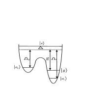
FIG. 1.: A schematic diagram of the energy level in the SQUID coupled to the single mode cavity field (with coupling constant $g$) and two microwave pulses (with coupling constants $\Omega_{0}$ and $\Omega_{1}$). The 3-photon resonance condition is satisfied and $\Delta$ is the detuning.

Regarding single-qubit operations, our scheme is similar to that proposed in [4, 5]. We choose the states $\left|a_{0}\right\rangle$ and $\left|a_{1}\right\rangle$ as the computational basis and $\left|g\right\rangle$ as an ancillary state. When $\Omega_{0}=\Omega_{1}=0$, the states $\left|a_{i}\right\rangle\left|0\right\rangle_{c}$ ($i=0,1$) span an eigenspace of the Hamiltonian (3) with zero eigenvalue., where, $\left|0\right\rangle_{c}$ is the vacuum state of the cavity field. If the cavity is cooled to zero temperature and the quantum gate operations are switched off, i.e., the Rabi frequencies of all the classical microwave pulses are set to zero, the state $\alpha\left|a_{0}\right\rangle+\beta\left|a_{1}\right\rangle$ of the qubit is isolated from the state of the cavity and does not change with time. When the Rabi frequencies $\Omega_{0}$ and $\Omega_{1}$ change adiabatically along a close path $C$ in the parameter space $M$ and return the point corresponding to $\Omega_{0}=\Omega_{1}=0$ (we refer to this point as $O$), an initial state $\left|\Psi_{0}\right\rangle=\left(\alpha\left|a_{0}\right\rangle+\beta\left|a_{1}\right\rangle\right)\left|0\right\rangle_{c}$ of the qubit-cavity composite system evolves according to the rule $\left|\Psi_{0}\right\rangle\rightarrow U\left(C\right)\left|\Psi_{0}\right\rangle$ [5, 21]. Here, $U\left(C\right)=P\exp\int_{C}A$ is the non-Abelian holonomy associated with the path $C$ and $A=\sum_{\mu}A_{\mu}d\lambda_{\mu}$ is the $U\left(2\right)$-valued connection expressed as $A_{\mu}^{ij}=\left\langle D_{i}\left(\lambda\right)\right|\frac{\partial}{\partial\lambda_{\mu}}\left|D_{j}\left(\lambda\right)\right\rangle$ where $\left\{\lambda_{\mu}\right\}$ are the coordinates of the parameter space $M$ and $\left|D_{i}\left(\lambda\right)\right\rangle$ ($i=0,1$) the basis of the eigenspace of the Hamiltonian (3) with zero eignevalue (hereafter we refer to the basis as dark states). Since the holonomy $U\left(C\right)$ is a unitary transformation in the space spanned by the states $\left|a_{0}\right\rangle\left|0\right\rangle_{c}$ and $\left|a_{1}\right\rangle\left|0\right\rangle_{c}$, it can actually be considered as a unitary transformation that only acts on the qubit state which is the superposition of $\left|a_{0}\right\rangle$ and $\left|a_{1}\right\rangle$.

Without loss of generality, we assume that the coupling coefficient $g$ is real and positive, and choose $\Omega_{0}=g\tan\left(\xi\right)e^{i\phi_{0}}$and $\Omega_{1}=g\tan\left(\theta\right)\sec\left(\xi\right)e^{i\phi_{1}}$ where $\theta,\xi\in\left[0,\frac{\pi}{2}\right)$ and $\phi_{i}\in\left[0,2\pi\right)$ $\left(i=0,1\right)$. We take the angles $\xi$, $\theta$, $\phi_{0}$ and $\phi_{1}$ as the coordinates of the parameter space $M$. The dark states of this invariant subspace spanned by the states $\{\left|a_{i}\right\rangle\left|0\right\rangle_{c}$, $\left|g\right\rangle\left|1\right\rangle_{c}$, $\left|e\right\rangle\left|0\right\rangle_{c}\}$ of the Hamiltonian (3) can be written as the vector functions in $M$: $\left|D_{0}\right\rangle=\cos\left(\xi\right)\left|a_{0}\right\rangle\left|0\right\rangle_{c}-\sin\left(\xi\right)e^{i\phi_{0}}\left|g\right\rangle\left|1\right\rangle_{c}$ and $\left|D_{1}\right\rangle=-\sin\left(\theta\right)\sin\left(\xi\right)e^{i\left(\phi_{1}-\phi_{0}\right)}\left|a_{0}\right\rangle\left|0\right\rangle_{c}-\sin\left(\theta\right)\cos\left(\xi\right)e^{i\phi_{1}}\left|g\right\rangle\left|1\right\rangle_{c}+\cos\left(\theta\right)\left|a_{1}\right\rangle\left|0\right\rangle_{c}.$ We wish to point out that our choices of the coordinates and dark states are quite different from those in Refs. [4, 5]. Here, the dark states $\left|D_{0}\right\rangle$ and $\left|D_{1}\right\rangle$ are single-valued at the point $O$ ($\theta=\xi=0$), e.g. $\left|D_{i}\left(O\right)\right\rangle=\left|a_{i}\right\rangle\left|0\right\rangle_{c}$.

It is well known that any single-qubit gate operation can be decomposed into the product of rotations about axies $z$ and $y$: $R_{z}\left(\varphi\right)=e^{i\varphi\sigma_{z}}$ and $R_{y}\left(\varphi\right)=e^{i\varphi\sigma_{y}}$, where, $\varphi$ is the angle, $\sigma_{z}$, and $\sigma_{y}$ are Pauli matrices defined as $\sigma_{y}=i\left(\left|a_{1}\right\rangle\left\langle a_{0}\right|-\left|a_{0}\right\rangle\left\langle a_{1}\right|\right)$ and $\sigma_{z}=\left(\left|a_{0}\right\rangle\left\langle a_{0}\right|-\left|a_{1}\right\rangle\left\langle a_{1}\right|\right)$. Therefore, we need only to show the realization of $R_{z}\left(\varphi\right)$ and $R_{y}\left(\varphi\right)$. To realize the gate $R_{y}\left(\varphi\right)$, we let the phases $\phi_{0}=\phi_{1}=0$. The $U\left(2\right)$ valued connections can be derived as $A_{\xi}=-i\sin\left(\theta\right)\sigma_{y}$, and $A_{\theta}=0$. After an adiabatic evolution along a closed path $C$ in the parameter space $M$, the related unitary transformation (holonomy) is just the rotation about $y$ axis $U\left(C\right)=\exp\left[i\varphi\left(C\right)\sigma_{y}\right]$, where the angle $\varphi\left(C\right)=-\left(\int_{C}\sin\left(\theta\right)d\xi\right)$ is dependent of the loop $C$. To achieve the gate $R_{z}\left(\varphi\right)$, we can set $\phi_{0}=\xi=0$ (i.e. $\Omega_{0}=0$) and change $\theta$ and $\phi_{1}$ adiabatically. In this case, the non-zero connection is $A_{\phi_{1}}=i\frac{1}{2}\sin^{2}\left(\theta\right)\left(1-\sigma_{z}\right)$. As a result, the holonomy associated with a close path $C$ can be written as $U\left(C\right)=e^{-i\chi\left(C\right)}e^{i\chi\left(C\right)\sigma_{z}}$ where $\chi\left(C\right)=-\frac{1}{2}\int\sin^{2}\left(\theta\right)d\phi_{1}$. It is easy to see that $U\left(C\right)$ is just a rotation about $z$ axis up to a global phase.

We now illustrate how to realize the controlled-PHASE gate as well as the controlled-NOT gate via the non-Abelian holonomy in the present system of SQUID qubits, which is the main and novel result of the present paper. At this stage, we consider the (3+1)-type energy-level structure of two rf-SQUIDs in a microwave cavity. We assume that the $\left|e\right\rangle\longleftrightarrow\left|g\right\rangle$ transition of each SQUID is coupled to the single mode cavity field. Also, we set the level spacing $\omega_{ei}$ between the states ($\left|e\right\rangle$, $\left|a_{i}\right\rangle,$ $i=0,1$) to be different. The transitions $\left|e\right\rangle\longleftrightarrow\left|a_{0}\right\rangle$ (or $\left|a_{1}\right\rangle$) in both SQUIDs are coupled to two distinguishable classical microwave pulses with different frequencies [15] and the ”3-photon resonance” condition of each SQUID is set to be satisfied. The Hamiltonian of such SQUIDs in a microwave cavity may be written as

$$H = \sum_{l=1,2}\left[\Omega_{0}^{\left(l\right)}\left|e\right\rangle_{l}\left\langle a_{0}\right|+\Omega_{1}^{\left(l\right)}\left|e\right\rangle_{l}\left\langle a_{1}\right|+h.c\right]$$ (5)

$$+\sum_{l=1,2}\left[g^{\left(l\right)}a\left|e\right\rangle_{l}\left\langle g\right|+h.c\right]+\sum_{l=1,2}\Delta^{\left(l\right)}\left|e\right\rangle_{l}\left\langle e\right|.$$

Here, $\Delta^{\left(l\right)}=\omega_{eg}^{\left(l\right)}-\omega_{c}^{\left(l\right)}=\omega_{ei}^{\left(l\right)}-\omega_{i}^{\left(l\right)}$ is the detunning of the $l$-th SQUID and $\Omega_{i}^{\left(l\right)}$ is the Rabi frequency of the microwave pulse coupled to the transition $\left|e\right\rangle_{l}\leftrightarrow\left|a_{i}\right\rangle_{l}$ of the $l$-th SQUID.

We still choose the states $\left|a_{i}\right\rangle_{l}$ $i=0,1$ as the computational basis of the $l$-th qubit. The two SQUIDs are coupled indirectly via the single mode cavity field. As in the previous discussions for the single-qubit gate case, it is seen that when all of the Rabi frequencies $\Omega_{i}^{\left(l\right)}$ of the classical microwave pluses are set to zero and the cavity is cooled to zero temperature, the two-qubit state, which can be written in terms of $\left|a_{i}\right\rangle_{1}\left|a_{j}\right\rangle_{2}$, is isolated from the state of the cavity and does not change with time. In the following, we show that the holonomy, associated with the adiabatic evolution of $\Omega_{i}^{\left(l\right)}$ along a closed path $C$ starting from the point $\Omega_{i}^{\left(l\right)}=0$ (we also refer to this point as $O$) in the parameter space $M$, can be used to achieve a controlled-PHASE gate or a controlled-NOT gate of the two qubits.

We first choose $\Omega_{0}^{\left(l\right)}=g^{\left(1\right)}\tan\left[\xi^{\left(l\right)}\right]e^{i\phi_{0}^{\left(l\right)}}$ and $\Omega_{1}^{\left(l\right)}=g^{\left(2\right)}\tan\left[\theta^{\left(l\right)}\right]\sec\left[\xi^{\left(l\right)}\right]e^{i\phi_{1}^{\left(l\right)}}$ ( $l=1,2$), and take $\xi^{\left(l\right)}$, $\phi_{0}^{\left(l\right)}$, $\theta^{\left(l\right)}$ and $\phi_{1}^{\left(l\right)}$ as the independent coordinates in the parameter space $M$. To realize the controlled-PHASE gate, we set $\theta^{\left(l\right)}=\phi_{1}^{\left(l\right)}=\phi_{0}^{\left(1\right)}=0$. This means that we set the Rabi frequencies $\Omega_{1}^{\left(1\right)}$ and $\Omega_{1}^{\left(2\right)}$ to zero and only change $\Omega_{0}^{\left(1\right)}$ and $\Omega_{0}^{\left(2\right)}$ adiabatically. It is found that the subspace spanned by the states $\left|a_{i}\right\rangle_{1}\left|a_{j}\right\rangle_{2}\left|0\right\rangle_{c}$, $\left|a_{i}\right\rangle_{1}\left|g\right\rangle_{2}\left|1\right\rangle_{c}$, $\left|g\right\rangle_{1}\left|g\right\rangle_{2}\left|2\right\rangle_{c}$, $\left|g\right\rangle_{1}\left|a_{i}\right\rangle_{2}\left|1\right\rangle_{c}$, $\left|e\right\rangle_{1}\left|a_{i}\right\rangle_{2}\left|0\right\rangle_{c}$, $\left|a_{i}\right\rangle_{1}\left|e\right\rangle_{2}\left|0\right\rangle_{c}$, $\left|e\right\rangle_{1}\left|g\right\rangle_{2}\left|1\right\rangle_{c}$, $\left|g\right\rangle_{1}\left|e\right\rangle_{2}\left|1\right\rangle_{c}$ and $\left|e\right\rangle_{1}\left|e\right\rangle_{2}\left|0\right\rangle_{c}$ $\left(i,j=0,1\right)$ is an invariance subspace (we call it as the subspace $I$) of the Hamiltonian (5). After some tedious derivations, the dark states, i.e. the basis of the eigenspace of Hamiltonian (5) with zero eigenvalue, can be obtained as:

$$\left|D_{00}\right\rangle = \Lambda_{00}^{-1}[\sin\left[\xi^{\left(1\right)}\right]\sin\left[\xi^{\left(2\right)}\right]e^{i\phi_{0}^{\left(2\right)}}\left|g\right\rangle_{1}\left|g\right\rangle_{2}\left|2\right\rangle_{c}$$ (9)

$$-\sqrt{2}\cos\left[\xi^{\left(1\right)}\right]\sin\left[\xi^{\left(2\right)}\right]e^{i\phi_{0}^{\left(2\right)}}\left|a_{0}\right\rangle_{1}\left|g\right\rangle_{2}\left|1\right\rangle_{c}$$

$$+\sqrt{2}\cos\left[\xi^{\left(1\right)}\right]\cos\left[\xi^{\left(2\right)}\right]\left|a_{0}\right\rangle_{1}\left|a_{0}\right\rangle_{2}\left|0\right\rangle_{c}$$

$$-\sqrt{2}\sin\left[\xi^{\left(1\right)}\right]\cos\left[\xi^{\left(2\right)}\right]\left|g\right\rangle_{1}\left|a_{0}\right\rangle_{2}\left|1\right\rangle_{c}]$$

$$\left|D_{01}\right\rangle = \cos\left[\xi^{\left(1\right)}\right]\left|a_{0}\right\rangle_{1}\left|a_{1}\right\rangle_{2}\left|0\right\rangle_{c}$$ (11)

$$-\sin\left[\xi^{\left(1\right)}\right]\left|g\right\rangle_{1}\left|a_{1}\right\rangle_{2}\left|1\right\rangle_{c}$$

$$\left|D_{10}\right\rangle = \cos\left[\xi^{\left(2\right)}\right]\left|a_{1}\right\rangle_{1}\left|a_{0}\right\rangle_{2}\left|0\right\rangle_{c}$$ (13)

$$-\sin\left[\xi^{\left(2\right)}\right]e^{i\phi_{0}^{\left(2\right)}}\left|a_{1}\right\rangle_{1}\left|g\right\rangle_{2}\left|1\right\rangle_{c}$$

$$\left|D_{11}\right\rangle = \left|a_{1}\right\rangle_{1}\left|a_{1}\right\rangle_{2}\left|0\right\rangle_{c}$$ (14)

where $\Lambda_{00}=\sqrt{2-\sin^{2}\left[\xi^{\left(1\right)}\right]\sin^{2}\left[\xi^{\left(2\right)}\right]}$. It is obvious that at the point $O$ where $\xi^{\left(1\right)}=\xi^{\left(2\right)}=0$, the above dark states are single valued: $\left|D_{ij}\left(O\right)\right\rangle=\left|a_{i}\right\rangle_{1}\left|a_{j}\right\rangle_{2}\left|0\right\rangle_{c}$ for $i,j=0,1$. The non-zero elements of $U\left(4\right)$-valued connections are just $A_{\phi_{0}^{\left(2\right)}}^{00,00}=i\Lambda_{00}^{-2}\left\{2-\sin^{2}\left[\xi^{\left(1\right)}\right]\right\}\sin^{2}\left[\xi^{\left(2\right)}\right]$ and $A_{\phi_{0}^{\left(2\right)}}^{10,10}=i\sin^{2}\left[\xi^{\left(2\right)}\right].$ When the system evolves adiabatically along a closed path $C$ in the parameter space $M$ and returns to the point $O$, the associated holonomy can be written as $U\left(C\right)=e^{i\eta\left(C\right)\left|a_{0}\right\rangle_{2}\left\langle a_{0}\right|}e^{i\phi\left(C\right)\left|a_{0}a_{0}\right\rangle\left\langle a_{0}a_{0}\right|}$. Here, the angles $\eta\left(C\right)$ and $\phi\left(C\right)$ are defined as $\phi\left(C\right)=\int\Lambda_{00}^{-2}\left[2-\sin^{2}\left[\xi^{\left(1\right)}\right]-\Lambda_{00}^{2}\right]\sin^{2}\left[\xi^{\left(2\right)}\right]d\phi_{0}^{\left(2\right)}$ and $\eta\left(C\right)=\int\sin^{2}\left[\xi^{\left(2\right)}\right]d\phi_{0}^{\left(2\right)}.$ In the above expression of $U\left(C\right)$, $\left|a_{0}\right\rangle_{2}\left\langle a_{0}\right|$ is the projection operator of the second qubit to the state $\left|a_{0}\right\rangle_{2}$. It is easy to see that the holonomy $U\left(C\right)$ is the production of a control phase gate operation and a single-qubit rotation about the $z$ axis operated on the second qubit. When $\phi\left(C\right)\neq 0$, $U\left(C\right)$ is an nontrivial two-qubit operation. If we choose the path $C$ which satisfing $\eta\left(C\right)=0$, we can obtain an explicit control phase gate via the holonomy $U\left(C\right)=$ $e^{i\phi\left(C\right)\left|a_{0}a_{0}\right\rangle\left\langle a_{0}a_{0}\right|}$.

Moreover, we may also realize the controlled-NOT by setting $\theta^{\left(1\right)}=\phi_{0}^{\left(j\right)}=\phi_{1}^{\left(j\right)}=0$ and choose $\theta^{\left(2\right)}$, $\xi^{\left(1\right)}$ and $\xi^{\left(2\right)}$ as the control parameters. In this case, the dark states can also be obtained with some straightforward derivations, but have quite complicated forms (not presented here). Our main result is that, when $-\int_{C}\sin\left[\theta^{\left(2\right)}\right]d\xi^{\left(2\right)}-\theta\left(C\right)=\pi/2$, the holonomy associated with a closed path can be expressed as $U\left(C\right)=e^{-i\frac{\pi}{4}}R_{y}^{\left(2\right)}\left[\theta\left(C\right)\right]R_{z}^{\left(1\right)}\left(\frac{\pi}{4}\right)R_{z}^{\left(2\right)}\left(\frac{\pi}{4}\right)U_{CN}R_{z}^{\left(2\right)}\left(-\frac{\pi}{4}\right)$, where

$$U_{CN}=\left|a_{0}\right\rangle_{1}\left\langle a_{0}\right|\otimes I^{\left(2\right)}+\left|a_{1}\right\rangle_{1}\left\langle a_{1}\right|\otimes\sigma_{x}^{\left(2\right)}$$ (15)

is just the controlled-NOT operation. Here, $I^{\left(2\right)}$ is the identity operator of the second qubit and the angle $\theta\left(C\right)$ are defined as $\theta\left(C\right)=-\int_{C}\beta^{-1}\Lambda_{01}^{-1}\Lambda_{00}^{-3}\Lambda_{2}d\xi^{\left(2\right)}-\int_{C}\beta^{-1}\Lambda_{01}^{-1}\Lambda_{00}^{-3}\Lambda_{1}d\xi^{\left(1\right)}$, where $\Lambda_{00}$ is defined as before and the other coefficients are defined as $\Lambda_{01}=\sqrt{2-\sin^{2}\left[\xi^{\left(1\right)}\right]\cos^{2}\left[\xi^{\left(2\right)}\right]\sin^{2}\left[\theta^{\left(2\right)}\right]}$, $\alpha=-\left(1/2\right)\Lambda_{00}^{-1}\Lambda_{01}^{-1}\sin^{2}\left[\xi^{\left(1\right)}\right]\sin\left[2\xi^{\left(2\right)}\right]\sin\left[\theta^{\left(2\right)}\right]$ and $\beta=\sqrt{1+\alpha^{2}}.$ Therefore, up to a global phase factor, $U\left(C\right)$ is just the product of control not operation and some single-qubit rotations.

In most cases, the Hamiltonian (5) has a four-dimension engenspace with zero eigenvalue in the invariant subspace $I$. The basis of the eigenspace are just the dark states $\left|D_{ij}\right\rangle$. Nevertheless, it is pointed out that, in some very special cases, there may be accidental degeneracy in a sub-manifold (we call it the AD sub-manifold) of the parameter space $M$. In the AD sub-manifold, in addition to the dark states $\left|D_{ij}\right\rangle$, the Hamiltonian has another two eigenstates with zero eigenvalue and thus the dimension of the Hamiltonian’s eigenspace with zero eigenvalue is six rather than four. It is apparently that if the path of the adiabatic evolution of the Rabi frequencies cross the AD manifold, there might be a transition from the four dark states $\left|D_{ij}\right\rangle$ to the two external states. To avoid this kind of unwanted transition, we should control the evolution path of the Rabi frequencies in the parameter space $M$ be far away enough from the AD sub-manifold. On the other hand, since the evolution of the Rabi frequencies in $M$ is assumed to begin and end at the same point $O$ where all the Rabi frequencies are set to zero, the accidental degeneracy at $O$ should be avoided. This can be implemented by adjusting the coupling strength $g^{\left(l\right)}$ via controlling the position of the SQUIDs in the cavity, or the detuning $\Delta^{\left(l\right)}$ of each SQUID via changing the bias fields. For instance, if the conditions $\Delta^{\left(1\right)}=\Delta^{\left(2\right)}\neq 0,g^{\left(1\right)}=g^{\left(2\right)}$ or $\Delta^{\left(1\right)}=\Delta^{\left(2\right)}=0,g^{\left(1\right)}\neq g^{\left(2\right)}$ are satisfied, the accidental degeneracy at point $O$ can be avoided.

Since the dark states have a non-zero projection to the single or two photon states, the photon dissipation caused by the imperfection would tend to destroy the dark states. To evaluate the influence of the photon dissipation, the Schoredinger equation controlled by the effective Hamiltonian

$$H_{eff}=H\left(t\right)-i\left(\kappa/2\right)a^{\dagger}a$$ (16)

needs to be solved. Here, $H\left(t\right)$ is the Hamiltonian defined in Eq. (5) (or Eq. (3)), and $\kappa$ the photon decay rate. The dissipation term $-i\left(\kappa/2\right)a^{\dagger}a$ can be considered as a perturbation. As a result of the first order perturbation theory, the fidelity of the quantum gate operation, i.e., the probability of the ideal finial state, may be expressed as

$$F\approx 1-\kappa\int_{0}^{T}\left\langle n\right\rangle_{ph}dt$$ (17)

where $T$ is the operation time and $\left\langle n\right\rangle_{ph}=\left\langle\Psi\left(t\right)\right|a^{\dagger}a\left|\Psi\left(t\right)\right\rangle$ is the instantaneous expectation value of photon number. Therefore, the condition under which the influence of photon dissipation can be neglected is simply $\kappa\int_{0}^{T}\left\langle n\right\rangle_{ph}dt<<1$. On the other hand, since our scheme is based on the adiabatic evolution of the quantum states, the adiabatic condition should be satisfied, which can be expressed as $\tilde{\Omega}T>>1$, where $\tilde{\Omega}$ is the energy gap between the dark state and other eigenstates of the Hamiltonian [5]. Here, $\tilde{\Omega}$ has the same order of amplitude as the SQUID-cavity coupling constant $g$. In practical quantum gate operations, we always have $T\sim 10^{3}g^{-1}$. Then the condition $\kappa\int_{0}^{T}\left\langle n\right\rangle_{ph}dt<<1$ can be satisfied when $g/\kappa\gtrsim 10^{4}$. The coupling constant of the SQUID and the cavity available at present is $g\sim 1.8\times 10^{8}s^{-1}$ [15]. The high quality factor of the cavity $Q=10^{6}\sim 10^{8}$ might be achieved experimentally [22]. This will lead to $\kappa\int_{0}^{T}\left\langle n\right\rangle_{ph}dt\lesssim 10^{-2}$ and thus the fidelity $F\simeq 1$.

FIG. 2.: The fidelities of a control phase gate for the initial states $\left|a_{0}\right\rangle_{1}\left|a_{0}\right\rangle_{2}$ (solid line), $\left|a_{0}\right\rangle_{1}\left|a_{1}\right\rangle_{2}$ (dashed line), $\left|a_{1}\right\rangle_{1}\left|a_{0}\right\rangle_{2}$ (dotted line), and $\left|a_{1}\right\rangle_{1}\left|a_{1}\right\rangle_{2}$ (dashed-dotted line), where the quantity $n$ is defined by the relation $g/\kappa=10^{n}$.

Finally, let us look into in some detail a typical control phase gate operation discussed before. In this operation, we assume $g^{\left(1\right)}=2g^{\left(2\right)}=g=1.8\times 10^{8}s^{-1}$ and $\Delta^{\left(1\right)}=\Delta^{\left(2\right)}=0$. The amplitudes of the Rabi frequencies $\Omega_{0}^{\left(1\right)}$ and $\Omega_{0}^{\left(2\right)}$ are varied following the Gaussian functions of time: $\Omega_{0}^{\left(1\right)}=2.5ge^{-\left(\frac{t-3\tau}{\tau}\right)^{2}},\Omega_{0}^{\left(2\right)}=ge^{-\left(\frac{t-3\tau}{\tau}\right)^{2}}e^{i\phi_{0}^{\left(2\right)}\left(t\right)}$, where $\tau=144g^{-1}$. The phase $\phi_{0}^{\left(2\right)}\left(t\right)$ is set to be a hyperbolic tangent function of time: $\phi_{0}^{\left(2\right)}\left(t\right)=\pi\times\left[1+\text{tanh}\left(\frac{t}{0.75\tau}\right)\right]$. As in the above discussions, the control gate operation can be written as an unitary transformation $U=e^{i\eta\left|a_{0}\right\rangle_{2}\left\langle a_{0}\right|}e^{i\phi\left|a_{0}a_{0}\right\rangle\left\langle a_{0}a_{0}\right|}$, where $\phi\approx\pi/6$ and $\eta\approx 4$. The operation time of this gate is about $8\times 10^{2}g^{-1}$. We estimate the fidelity of this operation using Eq. (17). In Fig. 2, the fidelity of the quantum gate operation with four possible initial states are plotted as a function of the ratio $g/\kappa$. It is seen that when $g/\kappa\sim 10^{3}-10^{4}$, the fidelity is larger than $90\%$. In particular, whenever $g/\kappa\sim 10^{5}$, the fidelity is improved to reach $99\%$.

We thank P. Zanardi and Y. Li for useful discussions. We also thank Prof. Siyuan-Han for his grate suggestion on the utilization of rf-SQUID whose effective potential is triple well. The work was supported by the RGC grant of Hong Kong (HKU7114/02P), the CRCG grant of HKU, the NSFC, the knowledge Innovation Program (KIP) of the Chinese Academy of Sciences, and the National Fundamental Research Program of China (001CB309310).

REFERENCES

• [1] P. Zanardi and M. Rasetti, Phys. Lett. A 264, 94 (1999), J. Pachos, P. Zanardi and M. Rasetti, Phys. Rev. A 61, 010305 (1999).
• [2] J. A. Jones, V. Vedral, A. Ekert, G. Castagnoli, Nature (London) 403, 869 (1999).
• [3] G. Falci, R. Fazo, G. M. Palma, J. Siewert and V. Vedral, Nature (London) 407, 355 (2000).
• [4] L. M. Duan, J. I. Cirac, and P. Zoller, Science 292, 1695 (2001).
• [5] A. Recati, T. Calarco, P. Zanardi, J. I. Cirac and P. Zoller, Phys. Rev. A 66, 032309 (2002).
• [6] S. L. Zhu and Z. D. Wang, Phys. Rev. Lett. 89, 097902 (2002); Phys. Rev. A 66, 042322 (2002).
• [7] J. Du et al., quant-ph/0207022.
• [8] L. Faoro, J. Siewert and R. Fazio, Phys. Rev. Lett. 90, 028301 (2003).
• [9] C. P. Sun, P. Zhang and Y. Li, LANAL eprint quant-ph/0311052; Y. Li, P. Zhang, P. Zanardi and C. P. Sun, quant-ph/0402177.
• [10] S. L. Zhu and Z. D. Wang, Phys. Rev. Lett 91, 187902 (2003).
• [11] Z. Kis and E. Paspalakis, Phys. Rev. B 69, 024510 (2004).
• [12] E. Paspalakis and N. J. Kylstra, Jour. Mod. Opt. 20 1679 (2004).
• [13] R. Migliore and A. MessinaPhys, Phys. Rev. B67 134505 (2003).
• [14] S. L. Zhu, Z. D. Wang and K. Yang, Phys. Rev. A 68, 034303 (2003).
• [15] C. P. Yang, S. I. Chu and S. Han, Phys. Rev. Lett. 92, 117902 (2004).
• [16] S. L. Zhu, Z. D. Wang and P. Zanardi, quant-ph/0403004.
• [17] Y. B. Gao, C. Li and C. P. Sun, LANAL eprint, quant-ph/0402172.
• [18] J. Q. You and F. Nori, Phys. Rev. B 68, 064509 (2003); J. Q. You and F. Nori, Physica E 18, 33 (2003).
• [19] Y. X. Liu, L. F. Wei and F. Nori, LANAL eprint, quant-ph/0402189.
• [20] S. Han, R. Rouse and J. E. Lukens, Phys. Rev. Lett. 76, 3404 (1996).
• [21] F. Wilczek and A. Zee, Phys. Rev. Lett. 52, 2111 (1984).
• [22] P.K. Day, H. G. LeDuc, B. Mazin, A. Vayonakis, and J. Zmuidzinas, Nature (London) 425, 817 (2003).