Quantum phase transitions and bipartite entanglement

Abstract

We develop a general theory of the relation between quantum phase transitions (QPTs) characterized by nonanalyticities in the energy and bipartite entanglement. We derive a functional relation between the matrix elements of two-particle reduced density matrices and the eigenvalues of general two-body Hamiltonians of $d$-level systems. The ground state energy eigenvalue and its derivatives, whose non-analyticity characterizes a QPT, are directly tied to bipartite entanglement measures. We show that first-order QPTs are signalled by density matrix elements themselves and second-order QPTs by the first derivative of density matrix elements. Our general conclusions are illustrated via several quantum spin models.

Recently, a great deal of effort has been devoted to the understanding of the connections between quantum information Chuang:book and the theory of quantum critical phenomena Sachdev:book . A key novel observation is that quantum entanglement can play an important role in a quantum phase transition (QPT) Osterloh:02 ; Osborne:02 ; JVidal:04a ; Huang:04 ; Vidal:03 ; Vidal:04 ; Verstraete:04a ; Barnum:04 ; Somma:04 ; Bose:02 ; Alcaraz:03 ; JVidal:04 ; Gu:03 ; Lambert:04 . In particular, for a number of spin systems, it has been shown that QPTs are signalled by a critical behavior of bipartite entanglement as measured, for instance, in terms of the concurrence Wootters:98 . For the case of second-order QPTs (2QPTs), the critical point was found to be associated to a singularity in the derivative of the ground state concurrence, as first illustrated, for the transverse field Ising chain, in Ref. Osterloh:02 , and generalized in Refs. Osborne:02 ; JVidal:04a ; Huang:04 (see Refs. Verstraete:04a ; Barnum:04 ; Somma:04 ; Vidal:03 ; Vidal:04 for an analysis in terms of other entanglement measures). In the case of first-order QPTs (1QPTs), discontinuities in the ground state concurrence were shown to detect the QPT Bose:02 ; Alcaraz:03 ; JVidal:04 . The studies conducted to date are based on the analysis of particular many-body models. Hence the general connection between bipartite entanglement and QPTs is not yet well understood. The aim of this work is to discuss, in a general framework, how bipartite entanglement can be related to a QPT characterized by nonanalyticities in the energy.

Expectation values and the reduced density matrix.— The most general Hamiltonian of non-identical particles, up to two-body interactions, reads

$$H=\sum_{i\alpha\beta}\epsilon_{\alpha\beta}^{i}\left|\alpha_{i}\right\rangle\left\langle\beta_{i}\right|+\sum_{ij\alpha\beta\gamma\delta}V_{\alpha\beta\gamma\delta}^{ij}\left|\alpha_{i}\right\rangle\left|\beta_{j}\right\rangle\left\langle\gamma_{i}\right|\left\langle\delta_{j}\right|,$$ (1)

where $\{\left|\alpha_{i}\right\rangle\}$ is a basis for the Hilbert space, $\alpha,\beta,\gamma,\delta\in\{0,1,...,d-1\}$, and $i,j$ enumerate $N$ “qudits” ($d$-level systems). Let $E=\langle\psi|H|\psi\rangle$ be the energy in a non-degenerate eigenstate $\left|\psi\right\rangle$ of the Hamiltonian. The two-spin reduced density operator ${\hat{\rho}}^{ij}$ is given by ${\hat{\rho}}^{ij}=\sum_{m}\left\langle m|\psi\right\rangle\left\langle\psi|m\right\rangle$, with $m$ running over all the $d^{N-2}$ orthonormal basis vectors, excluding qudits $i$ and $j$. ${\hat{\rho}}^{ij}$ has a $d^{2}\times d^{2}$ matrix representation ${\rho}^{ij}$, with elements ${\rho}_{\gamma\delta\alpha\beta}^{ij}=\left\langle\gamma_{i}\delta_{j}\right|{\hat{\rho}}^{ij}\left|\alpha_{i}\beta_{j}\right\rangle=\sum_{m}\left\langle\gamma_{i}\delta_{j}m|\psi\right\rangle\left\langle\psi|m\alpha_{i}\beta_{j}\right\rangle=\sum_{m}\left\langle\psi|m\alpha_{i}\beta_{j}\right\rangle\left\langle\gamma_{i}\delta_{j}m|\psi\right\rangle=\left\langle\psi|\alpha_{i}\beta_{j}\right\rangle\left\langle\gamma_{i}\delta_{j}|\psi\right\rangle$, where we have used that $\left\langle\psi|m\alpha_{i}\beta_{j}\right\rangle$ are $c$-numbers and $\sum_{m}\left|m\right\rangle\left\langle m\right|=1$. Similarly, we can show that ${\hat{\rho}}^{i}=\mathrm{Tr}_{j}({\hat{\rho}}^{ij})$ has a $d\times d$ matrix representation ${\rho}^{i}$ with elements $\rho_{\beta\alpha}^{i}=\left\langle\beta_{i}\right|{\hat{\rho}}^{i}\left|\alpha_{i}\right\rangle=\left\langle\psi|\alpha_{i}\right\rangle\left\langle\beta_{i}|\psi\right\rangle$. Therefore, the energy $\langle\psi|H|\psi\rangle$ is

$$E(\rho^{ij})=\sum_{ij}\mathrm{Tr}(\mathbf{U}(ij){\rho}^{ij}\mathbf{)},$$ (2)

with $\mathbf{U}(ij)$ denoting a $d^{2}\times d^{2}$ matrix whose elements are $U_{\alpha\beta,\gamma\delta}(ij)=\epsilon_{\alpha\gamma}^{i}\delta_{\beta\delta}^{j}/N_{i}+V_{\alpha\beta\gamma\delta}^{ij}$, where $N_{i}$ is the number of qudits that qudit $i$ interacts with, and $\delta_{\beta\delta}^{j}$ is the Kronecker symbol on qudit $j$. Clearly, Eq. (2) holds not only for the Hamiltonian operator but for any observable. Indeed, it turns out that the expectation value (or eigenvalue, for an eigenstate) of any two-qudit observable in an arbitrary state $\left|\psi\right\rangle$ is a linear function of the matrix elements of two-spin reduced density matrices. Moreover, it is easy to show that Eq. (2) is also valid for a set of qudits with distinct dimensions and for an arbitrary $D$-fold degenerate energy level, where $\rho^{ij}=(1/D)\sum_{p=1}^{D}\rho^{ij}_{p}$, with $\rho^{ij}_{p}$ denoting the reduced density operator associated to the degenerate eigenstate $|\psi_{p}\rangle$. These results easily generalize to the case of a Hamiltonian containing $n$-body terms; e.g., for a three-body operator $\hat{O}$, $\left\langle\psi\right|\hat{O}\left|\psi\right\rangle=\sum_{ijk}\mathrm{Tr}(\mathbf{O}(ijk){\rho}^{ijk})$, etc., for higher-order interactions. The above results hold for any value of $d$. Here we are especially interested in $d=2$, i.e., the qubit case. We then use the standard basis $\left\{\left|00\right\rangle,\left|01\right\rangle,\left|10\right\rangle,\left|11\right\rangle\right\}$ for any pair $(i,j)$ of spins, and denote $\rho_{11}^{ij}=\left\langle 0_{i}0_{j}\right|{\hat{\rho}}^{ij}\left|0_{i}0_{j}\right\rangle$, $\rho_{12}^{ij}=\left\langle 0_{i}0_{j}\right|{\hat{\rho}}^{ij}\left|0_{i}1_{j}\right\rangle$, etc.

QPT and the reduced density operator.— QPTs are critical changes in the properties of the ground state of a many-body system due to modifications in the interactions among its constituents, occurring at low temperatures $T$ where the de Broglie thermal wavelength is greater than the classical correlation length of the thermal fluctuations (effectively $T=0$) Sachdev:book . Typically, such a change is induced as a parameter $\lambda$ in the system Hamiltonian $H(\lambda)$ is varied across a critical point $\lambda_{c}$. Because they occur at $T=0$, QPTs are purely driven by quantum fluctuations. They are associated with level crossings which, in many cases, lead to the presence of nonanalyticities in the energy spectrum. Specifically, a 1QPT is characterized by a finite discontinuity in the first derivative of the ground state energy. A 2QPT (or continuous QPT) is similarly characterized by a finite discontinuity, or divergence, in the second derivative of the ground state energy, assuming the first derivative is continuous. These characterizations are the $T=0$ limits of the classical definition of the corresponding phase transitions, given in terms of the free energy Reichl . There are QPTs where this is not the case Zanardi:2004 ; Yang:04 . One such example is the QPT in the antiferromagnetic XXZ model, where a critical anisotropy separates a gapless phase from a gapful phase. As shown in Ref. Yang:66 , the ground state energy and all of its derivatives with respect to the anisotropy are continuous at the critical point, despite the existence of the QPT. Moreover, other examples where QPTs are not directly related to nonanlyticities in the ground state energy include transitions caused by level crossings in the low-lying excited states Nomura:94 ; Tian:03 and those associated with topological order (e.g., in fractional quantum Hall liquids), which is not characterized by symmetry breaking Wen:04 . We shall consider in this Letter only QPTs characterized by nonanalytic behavior in the derivatives of the ground state energy.

Assume that $\epsilon_{\alpha\beta}^{i}$ and $V_{\alpha\beta\gamma\delta}^{ij}$ are smooth functions of a set $\left\{\lambda_{k}\right\}$ of couplings. If $\left|\psi\right\rangle$ is an eigenstate of the Hamiltonian then, using $\partial_{\lambda}\langle\psi\left|\psi\right\rangle=0\Rightarrow\partial_{\lambda}E=\left\langle\psi\right|\partial_{\lambda}H\left|\psi\right\rangle$, we have from Eq. (2):

$$\partial_{\lambda}\mathcal{E}(\rho^{ij})=(1/N)\sum_{ij}\mathrm{Tr}([\partial_{\lambda}\mathbf{U}(ij)]\rho^{ij}),$$ (3)

where $\mathcal{E}=E/N$. It follows immediately from Eq. (3) that $\sum_{ij}\mathrm{Tr}(\mathbf{U}(ij)[\partial_{\lambda}\rho^{ij}])=0$. The origin of a 1QPT can now be seen to be the discontinuity of one or more of the $\rho^{ij}$’s at the critical point. The second derivative, obtained directly from Eq. (3), reads

$$\frac{\partial^{2}\mathcal{E}(\rho^{ij})}{\partial\lambda^{2}}=\frac{1}{N}\sum_{ij}\left\{\mathrm{Tr}(\frac{\partial^{2}\mathbf{U}(ij)}{\partial\lambda^{2}}\rho^{ij})+\mathrm{Tr}(\frac{\partial\mathbf{U}(ij)}{\partial\lambda}\frac{\partial\rho^{ij}}{\partial\lambda})\right\}$$ (4)

Since $\mathbf{U}(ij)$ is a smooth function of $\left\{\lambda_{k}\right\}$ and $\rho^{ij}$ is finite at the critical point $\lambda=\lambda_{c},$ it can now similarly be seen that the origin of the discontinuity or singularity of $\partial^{2}\mathcal{E}(\rho^{ij})/\partial\lambda^{2}$ is due to the fact that one or more of the $\partial\rho^{ij}/\partial\lambda$’s diverge at the critical point.

QPTs from bipartite entanglement.— In order to discuss the role of bipartite entanglement in a QPT we need appropriate entanglement measures $M(\rho^{ij})$: monotonic functions ranging from $0$ (no entanglement) to $1$ (maximal entanglement), invariant under local operations and classical communication Chuang:book . We consider two such measures: (i) concurrence Wootters:98 : $C(\rho^{ij})=\max(\gamma_{1}^{ij}-\gamma_{2}^{ij}-\gamma_{3}^{ij}-\gamma_{4}^{ij},0)$, where the $\gamma_{\alpha}^{ij}$ are the square-roots, in decreasing order, of the eigenvalues of the operator $R(\rho^{ij})\equiv\rho^{ij}(\sigma_{y}\otimes\sigma_{y})\rho^{ij\ast}(\sigma_{y}\otimes\sigma_{y})$, where $\rho^{ij\ast}$ denotes complex conjugation of $\rho^{ij}$ in the standard basis $\left\{\left|00\right\rangle,\left|01\right\rangle,\left|10\right\rangle,\left|11\right\rangle\right\}$; (ii) negativity Vidal:02a : $\mathcal{N}(\rho^{ij})=2\,\max(0,-\min_{\alpha}(\mu_{\alpha}^{ij}))$, where $\mu_{\alpha}^{ij}$ are the eigenvalues of the partial transpose $\rho^{ij,T_{A}}$ of the density operator $\rho^{ij}$, defined as $\left\langle\alpha\beta\right|\rho^{T_{A}}\left|\gamma\delta\right\rangle=\left\langle\gamma\beta\right|\rho\left|\alpha\delta\right\rangle$.

It is now a simple matter to connect these measures to the appearance of a QPT. From Eq. (2) we have $E(\rho^{ij})=\sum_{ij}\mathrm{Tr}(\mathbf{U}(ij)\rho^{ij})=\sum_{ij}\mathrm{Tr}(\mathbf{U}^{T_{A}}(ij)\rho^{ij,T_{A}})$, where the matrix elements of $\mathbf{U}^{T_{A}}(ij)$ are $\left\langle\alpha\beta\right|\mathbf{U}^{T_{A}}\left|\gamma\delta\right\rangle=\left\langle\gamma\beta\right|\mathbf{U}\left|\alpha\delta\right\rangle$. Let $W^{ij}$ be the unitary matrix that diagonalizes $\rho^{ij,T_{A}}$. Then, using Eq. (3), we obtain

$$\frac{\partial\mathcal{E}(\rho^{ij})}{\partial\lambda}=\frac{1}{N}\sum_{ij}\sum_{\alpha=1}^{4}\left\{W^{ij}\frac{\partial\mathbf{U}^{T_{A}}(ij)}{\partial\lambda}W^{ij\dagger}\right\}_{\alpha\alpha}\mu_{\alpha}^{ij}.$$ (5)

Theorem 1

Assume conditions (a)-(c) below are satisfied. Then: a discontinuity in [discontinuity in or divergence of the first derivative of] the concurrence or negativity is both necessary and sufficient to signal a 1QPT [2QPT].

(a) The 1QPT [2QPT] is associated to a discontinuity in [discontinuity in or divergence of] the first [second] derivative of the ground state energy, which originates exclusively from the elements of $\rho^{ij}$ and not, for instance, from the sum in Eq. (3) [Eq. (4)] itself. Similarly, a discontinuity in [discontinuity in or divergence of the first derivative of] the concurrence or negativity originates exclusively from $\rho^{ij}$ and not from other operations such as max or min.

(b) In the case of a 1QPT [2QPT] the discontinuous matrix elements of $\rho^{ij}$ present in Eq. (3) [discontinuous or divergent $\partial\rho^{ij}/\partial\lambda$ present in Eq. (4)] do not either all accidentally vanish or cancel with other terms in the expression for [the first derivative of] the concurrence or negativity.

(c) In the case of a 1QPT [2QPT] the discontinuous matrix elements of $\rho^{ij}$ present in [discontinuous or divergent $\partial\rho^{ij}/\partial\lambda$ present in the first derivative of] the concurrence or negativity do not either all accidentally vanish or cancel with other terms in Eq. (3) [Eq. (4)].

Conditions (a)-(c) above are meant to exclude artificial/accidental occurrences of non-analyticity. They are meant to emphasize that the entanglement-QPT connection may directly come from the ground state reduced density matrix. When non-analyticities originating from the density operator are present in both the entanglement measure (or its derivatives) and the derivatives of the ground state energy, bipartite entanglement and QPTs signal each other. These observations are also the basis of the proof we now give.

Proof. 1QPT: If condition (a) is satisfied then a 1QPT must come from the discontinuity of one (or more) matrix elements of $\rho^{ij}$, as given by Eq. (3). Thus, taking into account condition (b), the 1QPT will be associated to a discontinuity in the concurrence or negativity, which is therefore a necessary condition for the 1QPT. Sufficiency: (i) Concurrence – Taking into account condition (a), if one (or more) of the eigenvalues $\gamma_{\alpha}^{ij}$ of $R(\rho^{ij})$ is discontinuous then one (or more) of the matrix elements of $\rho^{ij}$ must be discontinuous. Assuming condition (c), a 1QPT then follows from Eq. (3). (ii) Negativity – the negativity and $\partial\mathcal{E}(\rho^{ij})/\partial\lambda$ are both linear in $\min_{\alpha}(\mu_{\alpha}^{ij})$. Therefore if the coefficient in front of $\min_{\alpha}(\mu_{\alpha}^{ij})$ in Eq. (5) does not accidentally vanish, as ensured by condition (c), a discontinuous negativity signals the 1QPT.

2QPT: Considering Eq. (4), if condition (a) is satisfied then a 2QPT must come from the discontinuity in or divergence of one (or more) $\partial\rho^{ij}/\partial\lambda$, since all the $\rho^{ij}$ are assumed to be continuous for the case of a 2QPT. Thus, taking into account condition (b), the 2QPT will be associated to a discontinuity in or divergence of the first derivative of the concurrence or negativity, which is therefore a necessary condition for the 2QPT. On the other hand, we have $\partial_{\lambda}M(\rho^{ij})=\sum_{a,b=1}^{4}[\partial M(\rho^{ij})/\partial\rho_{ab}^{ij}]\partial_{\lambda}\rho_{ab}^{ij}$. Therefore, taking into account condition (a), discontinuity in or divergence of $[\partial M(\rho^{ij})/\partial\lambda]_{\lambda_{c}}$ must be caused by one or more of the $[\partial\rho_{ab}^{ij}/\partial\lambda]_{\lambda_{c}}$. Assuming condition (c), this singular behavior of $\partial\rho^{ij}/\partial\lambda$ is then a sufficient condition for a 2QPT, which follows from Eq. (4).   

Some further features following from this general analysis are: (1) If $[\partial M(\rho^{ij})/\partial\lambda]_{\lambda_{c}}$ diverges then the maximal entanglement will not occur at the critical point $\lambda_{c}$. (2) Concerning the behavior in the vicinity of the critical point: our results above show that the speed of divergence of both energy and the entanglement measures is dominated by the fastest among the $\partial\rho_{ab}^{ij}/\partial\lambda$ (as illustrated in Fig. 1). Therefore $\partial M(\rho^{ij})/\partial\lambda$ should have similar divergent properties to the second derivative of energy. This is indeed the behavior observed for the transverse field Ising model in Ref. Osterloh:02 . (3) Examples exist wherein the max/min evaluations required by the definition of bipartite entanglement measures generate a singularity related to the derivative of these measures, without an associated QPT Yang:04 ; condition (a) of our Theorem excludes such (artificial) singularities. Moreover max/min can also eliminate singularities, a possibility which is excluded from consideration through condition (c). Next we consider examples to illustrate our general formalism.

Frustrated two-leg spin-$1/2$ ladder.— The Hamiltonian for this model is $H_{\mathrm{ladder}}=\sum_{\left\langle ij\right\rangle}J_{ij}\overrightarrow{S}_{i}\cdot\overrightarrow{S}_{j}-h\sum\limits_{i=1}^{N}S_{i}^{z}$, where $\overrightarrow{S}_{i}$ is the spin operator vector at site $i$, the exchange interaction along the rungs is $J_{ij}=J_{R}$, and both the intra-chain nearest-neighbor and diagonal exchange interactions are $J_{ij}=J$. We further assume $J_{R}>\gamma J$, with $\gamma\approx 1.401$ Bose:02 . This model is exactly solvable and exhibits 1QPTs for $h_{c_{1}}=J_{R}$ and $h_{c_{2}}=J_{R}+2J$. An analysis of pairwise entanglement for this model can be found in Ref. Bose:02 . For $h<h_{c_{1}}$, and in the limit $N\rightarrow\infty$, the ground state is a tensor product of (entangled) singlets, $(|01\rangle-|10\rangle)/\sqrt{2}$, along the rungs. When $h_{c_{1}}<h<h_{c_{2}}$, the ground state consists of rungs which are alternately in singlet and (unentangled) $S^{z}=1$ triplet spin configurations, $|00\rangle$. For $h>h_{c_{2}}$, the ground state is a tensor product of all rungs in the $S^{z}=1$ triplet state. The density matrix elements of the rungs are characterized by the following step-function discontinuities at the two critical points:

$$\rho^{r_{i}}_{22} = \rho^{r_{i}}_{33}=-\rho^{r_{i}}_{32}=-\rho^{r_{i}}_{23}=\left\{\begin{array}[]{l}\frac{1}{2},\text{\thinspace\thinspace}h<h_{c_{i}}\\ 0,\text{\thinspace\thinspace}h\geq h_{c_{i}}\end{array}\right.$$ (8)

$$\rho^{r_{i}}_{11} = \left\{\begin{array}[]{l}0,\text{\thinspace\thinspace}h<h_{c_{i}}\\ 1,\text{\thinspace\thinspace\thinspace}h\geq h_{c_{i}}\end{array}\right.$$ (11)

where $r_{i}$, with $i=1,2$, denotes rungs that transition to the $S^{z}=1$ configuration at the critical point $h_{c_{i}}$. All other density matrix elements for the rungs vanish. The ground state of the system is two-fold degenerate when $h_{c_{1}}\leq h<h_{c_{2}}$. The density operator for a rung is then represented by a statistical mixture of the broken-symmetry states $\rho^{r_{1}}$ and $\rho^{r_{2}}$, with equal probabilities. Indeed, for a general value of $h$, we can write the rung density matrix as $\rho^{r}=(\rho^{r_{1}}+\rho^{r_{2}})/2$. Below $h_{c_{2}}$, the ground state energy is given by the sum of the energies of each rung, due to the fact that all couplings proportional to $J$ vanish when acting on a singlet. Using Eq. (2) the energy density can be then written, for $h<h_{c_{2}}$, as ${\cal E}=\frac{1}{2}[\frac{J_{R}}{4}(\rho^{r}_{11}-\rho^{r}_{22}-\rho^{r}_{33}+\rho^{r}_{44}+2(\rho^{r}_{32}+\rho^{r}_{23}))-h(\rho^{r}_{11}-\rho^{r}_{44})]$. For $h\geq h_{c_{2}}$, contributions of the $J$ sector must be considered in the expression above. However the quantity $\partial{\cal E}/\partial h$, which characterizes the 1QPTs in this model, can be obtained directly from Eq. (3) for any $h$, resulting in $\partial_{h}\mathcal{E}=-\frac{1}{2}\,\rho^{r}_{11}=-\frac{1}{4}(\rho^{r_{1}}_{11}+\rho^{r_{2}}_{11})$, where we have used that $\rho^{r}_{44}=0$. It then follows from Eq. (11) that $\partial_{h}\mathcal{E}$ is discontinuous at both $h_{c_{1}}$ and $h_{c_{2}}$. The same discontinuous behavior is immediately revealed in the bipartite entanglement of the spins sharing a rung. For these pairs a direct calculation shows that the negativity and concurrence (which here turn out to be equal) read $\mathcal{N}=C=1-\rho^{r}_{11}=1-\frac{1}{2}(\rho^{r_{1}}_{11}+\rho^{r_{2}}_{11})$, which, therefore, are discontinuous functions at both $h=h_{c_{1}}$ and $h=h_{c_{2}}$. We thus find the remarkably simple result $\partial\mathcal{E}/\partial h=(\mathcal{N}-1)/2$, which can also be seen as a general consequence of Eq. (5). This expression exemplifies how entanglement directly detects a 1QPT.

Permutation invariance and the transverse field Ising chain.— We consider now the case of Hamiltonians whose ground states are invariant under a permutation $P_{ik}$ of an arbitrary pair $(i,k)$ of spins. In this case $P_{ik}\left|\psi\right\rangle=\pm\left|\psi\right\rangle$ so that $\left|\psi\right\rangle\left\langle\psi\right|=P_{ki}P_{lj}\left|\psi\right\rangle\left\langle\psi\right|P_{lj}P_{ki}.$ Therefore, from the general expression for the two-spin reduced density operator ${\hat{\rho}}^{ij}$: $\left\langle\gamma_{i}\delta_{j}\right|\widehat{\rho}^{ij}\left|\alpha_{i}\beta_{j}\right\rangle=\sum_{m}\left\langle\gamma_{i}\delta_{j}m|\psi\right\rangle\left\langle\psi|m\alpha_{i}\beta_{j}\right\rangle=\sum_{m}\left\langle\gamma_{k}\delta_{l}m|\psi\right\rangle\left\langle\psi|m\alpha_{k}\beta_{l}\right\rangle=\left\langle\gamma_{k}\delta_{l}\right|\widehat{\rho}^{kl}\left|\alpha_{k}\beta_{l}\right\rangle$, i.e., $\rho^{ij}=\rho^{kl}$. If only a constant nearest-neighbor interaction is taken into account then $\mathbf{U}(i,i+1)=\mathbf{U}(j,j+1)=\mathbf{U}$ $(\forall\,i,j)$. Then, denoting $\rho_{i,i+1}=\rho_{j,j+1}=\rho$ $(\forall\,i,j)$, we have $\mathcal{E}(\rho)=\mathrm{Tr}(\mathbf{U}\rho)$. As a specific example, consider the transverse field Ising chain with constant nearest-neighbor interactions, whose Hamiltonian is $H=-J\sum_{i=1}^{N}(\lambda\sigma_{i}^{x}\sigma_{i+1}^{x}+\sigma_{i}^{z})$, where $N$ is the number of spins along the chain, $\sigma_{i}^{\alpha}$ are the Pauli operators for a spin at site $i$, and we use periodic boundary conditions. Setting $J=1$, we obtain from Eq. (2) that $\mathcal{E}(\rho)=-\left\langle\psi\right|\sigma^{z}\left|\psi\right\rangle-2\lambda(\rho_{14}+\rho_{23})$, where the site-independent ground state expectation value of $\sigma^{z}$ is $\left\langle\psi\right|\sigma^{z}\left|\psi\right\rangle=\rho_{11}-\rho_{44}$. This model presents a 2QPT at $\lambda_{c}=1$ Sachdev:book . This can be identified within our framework by taking the second derivative of $\mathcal{E}(\rho)$, yielding

$$\frac{\partial^{2}\mathcal{E}(\rho)}{\partial\lambda^{2}}=-2\frac{1}{\lambda}\frac{\partial}{\partial\lambda}(\rho_{22}+\rho_{44}),$$ (12)

where we used $\sum_{ij}\mathrm{Tr}(\mathbf{U}(ij)\frac{\partial\rho^{ij}}{\partial\lambda})=0$ and $\mathrm{Tr}\rho=1$. We have calculated the $\rho_{ij}$ using the standard method of fermionization and a Bogoliubov transformation Sachdev:book . At the critical point $\lambda_{c}$, Eq. (12) displays a divergence in the limit of an infinite chain. This 2QPT originates from the singular behavior of $\partial_{\lambda}\rho_{22}$ and $\partial_{\lambda}\rho_{44}$, as shown in Fig. 1. It is clear from this figure that $\partial_{\lambda}\rho_{22}$ is dominantly responsible for the divergence.

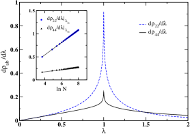
Figure 1: First derivative of elements of the two-spin reduced density matrix for the transverse field Ising model with $N=1000$ sites. Inset: $d\rho_{22}/d\lambda$ and $d\rho_{44}/d\lambda$ diverge logarithmically as a function of $N$. They are fitted by $x_{{\textrm{ab}}}\,{\textrm{ln}}\,N+const$, with $x_{22}=0.135$ and $x_{44}=0.024$.

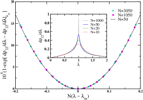
Figure 2: Finite size scaling of $\partial_{\lambda}\rho_{22}$ with the number $N$ of sites for the transverse field Ising chain. $\partial_{\lambda}\rho_{22}$ is a function of $N^{1/\nu}(\lambda-\lambda_{m})$ only, with the Ising model critical exponent $\nu=1$, and $\lambda_{m}$ being the position of the maximum of $\rho_{22}(N,\lambda)$. All the data from $N=50$ to $N=3050$ collapse onto a single curve. Inset: $\partial_{\lambda}\rho_{22}$ before scaling, showing increase in singular peak sharpness with $N$ and shift of $\lambda_{m}$.

Now, concerning the ground state nearest-neighbor bipartite entanglement, the global $\pi$-rotation invariance of the model about the spin $z$-axis ($Z_{2}$-symmetry) and a detailed computation of the density matrix elements leads to $C=\mathcal{N}=2(\rho_{41}-\rho_{22})$. As shown in Ref. Syl:03 , the concurrence in this case is not modified by spontaneous symmetry breaking. In the limit $N\rightarrow\infty$, $(\partial C/\partial\lambda)|_{\lambda_{c}}$ is logarithmically divergent Osterloh:02 . This result is here seen to be a direct consequence of the singular behavior of $\partial_{\lambda}\rho_{22}$, just as in the second derivative of energy, since $\partial_{\lambda}\rho_{41}$ is a smooth function of $\lambda$. Therefore $\partial^{2}\mathcal{E}/\partial\lambda^{2}$ and $\partial C/\partial\lambda$ exhibit similar critical behavior through their dependence upon $\partial\rho_{22}/\partial\lambda$, whose finite-size scaling is shown in Fig. 2. The conclusion of Osterloh:02 , that the concurrence detects the phase transition in the Ising model, is thus simply explained within our framework.

We gratefully acknowledge financial support from CNPq-Brazil (to M.S.S.), and the Sloan Foundation, PREA and NSERC (to D.A.L.). We thank Prof. L.-M. Duan and Dr. P. Zanardi for inspiring discussions and Dr. M.-F. Yang for useful correspondence.

References

(1) M. A. Nielsen and I. L. Chuang, Quantum Computation and
Quantum Information (Cambridge University Press, Cambridge, U.K., 2000).
(2)
S. Sachdev, Quantum Phase Transitions (Cambridge University Press,
Cambridge, U.K., 2001).
(3)
A. Osterloh, L. Amico, G. Falci, and R. Fazio, Nature 416, 608
(2002).
(4)
T. J. Osborne and M. A. Nielsen, Phys. Rev. A 66, 032110 (2002).
(5)
J. Vidal, G. Palacios, and R. Mosseri, Phys. Rev. A 69, 022107
(2004).
(6) Z. Huang, O. Osenda, and S. Kais, Phys. Lett. A 322,
137 (2004).
(7)
G. Vidal, J. I. Latorre, E. Rico, and A. Kitaev, Phys. Rev. Lett. 90,
227902 (2003).
(8)
J. I. Latorre, E. Rico, and G. Vidal, Quant. Inf. Comp. 4, 48 (2004).
(9)
F. Verstraete, M. Popp, and J. I. Cirac, Phys. Rev. Lett. 92, 027901
(2004).
(10)
H. Barnum, E. Knill, G. Ortiz, R. Somma, and L. Viola, Phys. Rev. Lett. 92, 107902 (2004).
(11)
R. Somma, G. Ortiz, H. Barnum, E. Knill, and L. Viola, Phys. Rev. A 70, 042311 (2004).
(12)
I. Bose and E. Chattopadhyay, Phys. Rev. A 66, 062320 (2002).
(13)
F. C. Alcaraz, A. Saguia, and M. S. Sarandy, Phys. Rev. A 70, 032333 (2004).
(14)
J. Vidal, R. Mosseri, and J. Dukelsky, Phys. Rev. A 69, 054101 (2004).
(15)
N. Lambert, C. Emary, and T. Brandes, Phys. Rev. Lett. 92, 073602
(2004).
(16)
S.-J. Gu, H.-Q. Lin, and Y.-Q. Li, Phys. Rev. A 68, 042330 (2003).
(17)
W. K. Wootters, Phys. Rev. Lett. 80, 2245 (1998).
(18) Y. Chen, P. Zanardi, Z. D. Wang, and F. C. Zhang,
e-print quant-ph/0407228 (2004).
(19) M.-F. Yang, e-print quant-ph/0407226 (2004).
(20) C. N. Yang and C. P. Yang, Phys. Rev. 150, 327 (1966).
(21) K. Nomura and K. Okamoto, J. Phys. A 27, 5773 (1994).
(22) G.-S. Tian and H.-Q. Lin, Phys. Rev. B 67, 245105 (2003).
(23) A. Hamma, P. Zanardi, and X.-G. Wen, e-print cond-mat/0411752.
(24)
L. E. Reichl, A Modern Course in Statistical Physics (John Wiley &
Sons, New York, 1998).
(25)
G. Vidal, R. F. Werner, Phys. Rev. A 65, 032314 (2002).
(26) O. F. Syljuåsen, Phys. Rev. A 68, 060301(R) (2003).