Implementation of Group-Covariant POVMs
by Orthogonal Measurements

Abstract

We consider group-covariant positive operator valued measures (POVMs) on a finite dimensional quantum system. Following Neumark’s theorem a POVM can be implemented by an orthogonal measurement on a larger system. Accordingly, our goal is to find an implementation of a given group-covariant POVM by a quantum circuit using its symmetry. Based on representation theory of the symmetry group we develop a general approach for the implementation of group-covariant POVMs which consist of rank-one operators. The construction relies on a method to decompose matrices that intertwine two representations of a finite group. We give several examples for which the resulting quantum circuits are efficient. In particular, we obtain efficient quantum circuits for a class of POVMs generated by Weyl-Heisenberg groups. These circuits allow to implement an approximative simultaneous measurement of the position and crystal momentum of a particle moving on a cyclic chain.

1 Introduction

General measurements of quantum systems are described by positive operator-valued measures (POVMs) [1, 2]. For several optimality criteria the use of POVMs can be advantageous as compared to projector valued measurements. This is true, e. g., for the mean square error, the minimum probability of error [3], and the mutual information [4]. POVMs are more flexible than orthogonal von Neumann measurements and can consist of finite as well as of an infinite number of elements. An example for the latter is given in [5] where a POVM for measuring the spin direction is proposed. Here we restrict our attention to the finite case where a POVM is described by a set of positive operators which sum up to the identity. Such a POVM is called group-covariant if the set is invariant under the action of a group. The example of POVMs for the Weyl-Heisenberg groups as well as the example in [5] show that POVMs are needed to describe phenomenologically the mesoscopic scale of quantum systems. They allow approximatively simultaneous measurements of quantum observables which are actually incompatible. For instance, the classical phase space of a particle can be approximatively reproduced by simultaneous measurements of momentum and position. Descriptions of quantum particles which have strong analogy to the classical phase space are helpful to understand the relations between the classical and the quantum world [6]. Also for several other tasks in quantum information processing the implementation of POVMs is of interest [7, 8, 9].

Neumark’s theorem [10, 11] states that in principle every POVM can be implemented by an orthogonal measurement of the joint system consisting of the system and an ancilla system. However, the orthogonal measurement required by this construction may not be a “natural” observable of the joint system. One may need an additional unitary transform to obtain a reduction to a more natural observable which henceforth will be called the measurement in the computational basis of the quantum system.

Therefore, the question arises how to actually implement a POVM in terms of a quantum circuit which itself is composed of a sequence of elementary quantum gates [12]. So far, only little is known about the implementation of POVMs even in quantum systems with a small number of dimensions. While some rather specific single-qubit measurements have been studied [4, 13, 14], not much is known about the general problem of how to implement a POVM by a unitary transform on the quantum register of a possibly larger space followed by an orthogonal measurement in the computational basis.

When studying quantum circuits for families of POVMs questions about the complexity of the required unitary transforms arise. In some cases we can exploit the fact that they admit some additional symmetry. This leads to the study of group-covariant POVMs which has been studied extensively in the literature [15, 4, 16, 17]. As a recent example we mention the construction of symmetric informationally complete POVMs by means of suitable finite symmetry groups [18].

The main contribution of this paper is a general method which computes an embedding of group-covariant POVMs into orthogonal measurements on a larger Hilbert space. A particular feature of the computed embedding is that it uses the symmetry. This in turn allows to apply known techniques for decomposing matrices with symmetry to the unitary matrices obtained by this embedding. For several cases this leads to families of efficient quantum circuits implementing the given POVMs.

Outline. In Section 2 we briefly recall the definition of POVMs. In Section 3 we consider the decomposition of matrices that have a symmetry with respect to a group. This type of decomposition is a basic tool for our constructions. We also define group-covariance of POVMs with respect to a symmetry group and a group representation. Furthermore, we explain how POVMs with this group-covariance are related to so-called monomial representations of the symmetry group. In Section 4 we explain the general scheme for the construction of a unitary transform that implements a group-covariant POVM. The basis for this construction is the analysis of the intertwining space between the group representation that is given by the group-covariance of the POVM and the monomial representation. This is the starting point for methods using fast quantum Fourier transforms as described in Section 5. Finally, in Section 6 we give several examples of implementations of group-covariant POVMs.

Notations. We denote the field of complex numbers by ${\mathbb{C}}$. The group of invertible $n\times n$ matrices is denoted by ${\rm GL}_{n}({\mathbb{C}})$ and the subgroup consisting the unitary $n\times n$ matrices is denoted by ${\cal U}(n)$. We denote the identity matrix in ${\cal U}(n)$ by $\mbox{\bf 1}_{n}$. If not denoted otherwise all matrices are matrices over the complex numbers. The cyclic group of order $n$ is denoted by ${\mathbb{Z}}_{n}$. Representations are denoted by small Greek letters, e. g., $\varphi$, $\psi$ etc. By abuse of notation we also denote the trivial representation of degree $n$ (i.e. dimension $n$) by $\mbox{\bf 1}_{n}$. The base change of a matrix $A$ with respect to a matrix $B$ is denoted by $A^{B}=BAB^{\dagger}$. The direct sum of matrices and representations is denoted by $A\oplus B$ and $\varphi\oplus\psi$ and the tensor product is denoted by $A\otimes B$ and $\varphi\otimes\psi$, respectively. We make frequent use of the Pauli matrices

$$\sigma_{x}=\left(\begin{array}[]{rr}0&1\\ 1&0\end{array}\right),\quad\sigma_{y}=\left(\begin{array}[]{rr}0&-i\\ i&0\end{array}\right),\quad\sigma_{z}=\left(\begin{array}[]{rr}1&0\\ 0&-1\end{array}\right).$$

A diagonal matrix with diagonal entries $\lambda_{1},\ldots,\lambda_{n}$ is abbreviated by ${\rm diag}(\lambda_{1},\ldots,\lambda_{n})$. We denote the symmetric group on $n$ symbols by ${\cal S}_{n}$. To each permutation $\sigma\in{\cal S}_{n}$ naturally corresponds the permutation matrix $\sum_{i}|\sigma(i)\rangle\langle i|$. By abuse of notation we identify $\sigma$ with the corresponding permutation matrix. We often use the permutation matrix $S_{m}$ which corresponds to the $m$-cycle $(1,2,\ldots,m)$ and the matrix $T_{m}={\rm diag}(1,\omega_{m},\ldots\omega_{m}^{m-1})$ which contains the eigenvalues of $S_{m}$. The basis states of an $n$-qubit system correspond to binary strings of length $n$. Quantum circuits are written from the left to the right, and the qubits are arranged such that the most significant qubit (characterizing the left-most symbol of a binary string) is on top. Throughout the paper a matrix entry “$\cdot$” stands for zero.

2 POVMs and orthogonal measurements

A POVM for a quantum system with Hilbert space ${\mathbb{C}}^{d}$ is a set $P=\{A_{1},\ldots,A_{n}\}\subseteq{\mathbb{C}}^{d\times d}$ of non-negative operators, where $\sum_{k}A_{k}=\mbox{\bf 1}_{d}$. For a more general definition for POVMs with an infinite number of operators we refer to [19]. For example, the set of matrices

$$P_{2}=\left\{\frac{1}{3}\left(\begin{array}[]{rr}1&1\\ 1&1\end{array}\right),\ \frac{1}{3}\left(\begin{array}[]{rr}1&\omega\\ \omega^{2}&1\end{array}\right),\ \frac{1}{3}\left(\begin{array}[]{rr}1&\omega^{2}\\ \omega&1\end{array}\right)\right\}\subseteq{\mathbb{C}}^{2\times 2},$$

where $\omega={\rm exp}(2\pi i/3)$ is a third root of unity, defines a POVM on a system with corresponding Hilbert space ${\mathbb{C}}^{2}$. Suppose that the state of the system is described by the density matrix $\rho\in{\mathbb{C}}^{d\times d}$. Then for a general POVM the probability $p_{k}$ for the result $k$ is given by $p_{k}={\rm tr}(\rho A_{k})$. An orthogonal measurement is a POVM with mutually orthogonal operators $A_{k}$, i. e., we have that $A_{k}A_{l}=A_{l}A_{k}=0$ for $k\not=l$.

In the following we restrict ourselves to rank-one operators $A_{k}=|\Psi_{k}\rangle\langle\Psi_{k}|$. Note that the POVM vectors $|\Psi_{k}\rangle$ need not be normalized and that the restriction to operators of rank one is for some applications justified by Davies’ theorem [15]. It states that we can always find a POVM with rank-one operators that maximizes the mutual information. The example $P_{2}$, which consists of three rank-one operators, can be written as $P_{2}=\{|\Psi_{1}\rangle\langle\Psi_{1}|,|\Psi_{2}\rangle\langle\Psi_{2}|,|\Psi_{3}\rangle\langle\Psi_{3}|\}$, where

$$|\Psi_{1}\rangle=\frac{1}{\sqrt{3}}\left(\begin{array}[]{c}1\\ 1\end{array}\right),\ |\Psi_{2}\rangle=\frac{1}{\sqrt{3}}\left(\begin{array}[]{c}1\\ \omega^{2}\end{array}\right),\quad{\rm and}\quad|\Psi_{3}\rangle=\frac{1}{\sqrt{3}}\left(\begin{array}[]{c}1\\ \omega\end{array}\right)$$

are the corresponding POVM vectors in ${\mathbb{C}}^{2}$. Neumark’s theorem [11] states that it is possible to implement a POVM by reducing it to an orthogonal measurement on a larger system. We briefly recall this construction. Let $P=\{A_{k}\}=\{|\Psi_{k}\rangle\langle\Psi_{k}|\}$ be a POVM with $n$ operators that acts on the Hilbert space ${\mathbb{C}}^{d}$. For $n>d$ the vectors $|\Psi_{k}\rangle$ cannot be mutually orthogonal. Consequently, we have to extend the system by at least $n-d$ dimensions in order to define an orthogonal measurement with $n$ different measurement outcomes. We want to implement an orthogonal measurement ${\tilde{P}}=\{{\tilde{A}}_{k}\}=\{|{\tilde{\Psi}}_{k}\rangle\langle{\tilde{\Psi}}_{k}|\}$ on the system with $n$ dimensions such that ${\tilde{P}}$ corresponds to the POVM $P$ on the subsystem with $d$ dimensions, i. e., $p_{k}={\rm tr}(\rho A_{k})={\rm tr}(\tilde{\rho}\tilde{A}_{k})$. Here ${\tilde{\rho}}=\rho\oplus 0_{n-d}\in{\mathbb{C}}^{n\times n}$ where $0_{n-d}$ denotes the zero matrix of size $n-d$ is the embedding of the state into the larger system.

We write the POVM vectors $|\Psi_{k}\rangle$ as columns of the matrix $M=\left(|\Psi_{1}\rangle\ldots|\Psi_{n}\rangle\right)\in{\mathbb{C}}^{d\times n}$. In the following we refer to $M$ as the defining matrix for the POVM $P$. Now, the operators ${\tilde{A}}_{k}=|{\tilde{\Psi}}_{k}\rangle\langle{\tilde{\Psi}}_{k}|\in{\mathbb{C}}^{n\times n}$ with $|{\tilde{\Psi}}_{k}\rangle=|\Psi_{k}\rangle\oplus|\Phi_{k}\rangle$ are the columns of the matrix

$${\tilde{M}}=\left(\begin{array}[]{ccc}|\Psi_{1}\rangle&\ldots&|\Psi_{n}\rangle\\ |\Phi_{1}\rangle&\ldots&|\Phi_{n}\rangle\end{array}\right)\in{\cal U}(n).$$

Note that $\tilde{M}$ can be an arbitrary unitary matrix which contains $M$ as upper part of size $d\times n$. Since $P$ is a POVM we have $MM^{\dagger}=\sum_{k}|\Psi_{k}\rangle\langle\Psi_{k}|=\sum_{k}A_{k}=\mbox{\bf 1}_{d}$, i. e., finding a suitable $\tilde{M}$ is always possible. For example in case of $P_{2}$ we obtain the defining matrix

$$M=\frac{1}{\sqrt{3}}\left(\begin{array}[]{ccc}1&1&1\\ 1&\omega^{2}&\omega\end{array}\right)\in{\mathbb{C}}^{2\times 3}$$

and one possible choice for $\tilde{M}$ is to add the row given by $(1/\sqrt{3})(1,\omega,\omega^{2})$. Hence the rank-one projectors corresponding to the orthogonal measurement ${\tilde{M}}$ are

$$|{\tilde{\Psi}}_{1}\rangle=\frac{1}{\sqrt{3}}\left(\begin{array}[]{c}1\\ 1\\ 1\end{array}\right),\ |{\tilde{\Psi}}_{2}\rangle=\frac{1}{\sqrt{3}}\left(\begin{array}[]{c}1\\ \omega^{2}\\ \omega\end{array}\right),{\rm and}\ \ |{\tilde{\Psi}}_{3}\rangle=\frac{1}{\sqrt{3}}\left(\begin{array}[]{c}1\\ \omega\\ \omega^{2}\end{array}\right).$$

The probability distribution ${\tilde{p}}_{k}={\rm tr}({\tilde{\rho}}{\tilde{A}}_{k})$ of the constructed orthogonal measurement equals the distribution $p_{k}$ of the original POVM since

$${\tilde{p}}_{k}={\rm tr}\left({\tilde{\rho}}{\tilde{A}}_{k}\right)={\rm tr}\left(\left(\rho\oplus 0_{n-d}\right)\left(\begin{array}[]{cc}|\Psi_{k}\rangle\langle\Psi_{k}|&|\Psi_{k}\rangle\langle\Phi_{k}|\\ |\Phi_{k}\rangle\langle\Psi_{k}|&|\Phi_{k}\rangle\langle\Phi_{k}|\end{array}\right)\right)={\rm tr}\left(\rho A_{k}\right)=p_{k}.$$

The embedding into a larger system can be realized by using an ancilla register of a quantum computer. It consists of $l$ qubits such that $2^{l}\geq n-d$. They are initially in the state $|0\dots 0\rangle$. Then the space ${\mathbb{C}}^{d}\otimes|0\dots 0\rangle$ is the subspace where the POVM acts on and ${\mathbb{C}}^{d}\otimes({\mathbb{C}}^{2})^{\otimes l}$ is the extension. The density operator $\tilde{\rho}$ acts on an $n$ dimensional subspace of the joint system consisting of the original system and the ancilla register. In the following we will assume that also the system space ${\mathbb{C}}^{d}$ is embedded into the state space of some qubits.

As explained above, we can implement the POVM with corresponding matrix $M$ by applying the unitary transform ${\tilde{M}}^{\dagger}$ to the initial state ${\tilde{\rho}}$ of the joint system followed by a measurement in the computational basis. Note that for the special case where the columns of $M$ are already orthogonal we have that ${\tilde{M}}=M$. In this case by implementing the matrix $M^{\dagger}$ followed by a measurement in the computational basis we can perfectly distinguish between the columns of $M$.

In principle, the construction of an appropriate matrix ${\tilde{M}}$ is simple since we just have to find mutually orthogonal rows that lead to a unitary matrix. However, $k$ qubits allow POVMs with $n=2^{k}$ operators. Hence the size of $\tilde{M}$ is exponential in $k$. The complexity to implement a unitary matrix on $k$ qubits can be upper bounded by $O(4^{k})$ [20] and a generic element of ${\cal U}(2^{k})$ will indeed require an exponential number of elementary transforms (e.g. one- and two-qubit-gates). Therefore we are interested in the construction of a matrix ${\tilde{M}}$ that can be implemented efficiently, if such a construction exists at all. While finding efficient factorizations is a hard problem in general, the situation becomes easier in some cases where we are given the additional structure of a group-covariant POVM. In the following sections we will give a definition of group-covariance and the related notion of symmetry. Later, we exploit the symmetry of the matrix $M$ and give several examples of POVMs that have efficient quantum circuit implementations.

3 Group-covariant POVMs and matrices with symmetry

In the following we give a precise mathematical definition of the notion of symmetry of a matrix $M\in{\mathbb{C}}^{m\times n}$. Later we define group-covariance of a POVM and show that the group-covariance in a natural way leads to matrices with symmetry. For the necessary background on finite groups and representations we refer to standard textbooks such as [21, 22].

We start with a finite group $G$ and a pair $(\varphi,\psi)$ of matrix representations of $G$ which are compatible with the size of $M$, i. e., $\varphi:G\to{\rm GL}_{m}({\mathbb{C}})$ and $\psi:G\to{\rm GL}_{n}({\mathbb{C}})$. Following, [23, 24] we call the triple $(G,\varphi,\psi)$ a symmetry of $M$ if the identity $\varphi(g)M=M\psi(g)$ holds for all $g\in G$. Sometimes we abbreviate this by using the shorthand notation $\varphi M=M\psi$. Note that if $M$ is not a square matrix the representations $\varphi$ and $\psi$ have different degrees.

To give an example we let $\omega=\exp(2\pi i/3)$ and let $\alpha,\beta,\gamma\in{\mathbb{C}}$. Then for all $j\in\{0,1,2\}$ we have that

$$\left(\begin{array}[]{ccc}1&\cdot&\cdot\\ \cdot&\omega&\cdot\\ \cdot&\cdot&\omega^{2}\end{array}\right)^{j}\left(\begin{array}[]{ccc}\alpha&\alpha&\alpha\\ \beta&\beta\omega&\beta\omega^{2}\\ \gamma&\gamma\omega^{2}&\gamma\omega\end{array}\right)=\left(\begin{array}[]{ccc}\alpha&\alpha&\alpha\\ \beta&\beta\omega&\beta\omega^{2}\\ \gamma&\gamma\omega^{2}&\gamma\omega\end{array}\right)\left(\begin{array}[]{ccc}\cdot&\cdot&1\\ 1&\cdot&\cdot\\ \cdot&1&\cdot\end{array}\right)^{j}.$$

Hence we obtain a symmetry which is given by the cyclic group ${\mathbb{Z}}_{3}=\{0,1,2\}$ together with the two representations $\varphi,\sigma:{\mathbb{Z}}_{3}\to{\cal U}(3)$ given by $\varphi(1)={\rm diag}(1,\omega,\omega^{2})$ and $\sigma(1)=(1,3,2)$.

Note that given two representations $\varphi$, $\psi$ of a group $G$ the set of all matrices $M$ which fulfill $\varphi(g)M=M\psi(g)$ for all $g\in G$ is a vector space. It turns out that the matrices in this vector space have a special form. Hence we explore its structure in more detail in the following.

Definition 1 (Intertwining space)

Let $G$ be a group and let $\varphi$, $\psi$ be representations of $G$ of degrees $n$ and $m$, respectively. Then

$${\rm Int}(\varphi,\psi):=\{M:\varphi(g)M=M\psi(g),\;\mbox{for all}\;g\in G\}$$

with $M\in{\mathbb{C}}^{n\times m}$ is called the intertwining space of $\varphi$ and $\psi$.

In the following we denote by $\varphi_{1},\ldots,\varphi_{k}$ a list of all pairwise inequivalent irreducible representations of $G$. Recall that for any representation of a finite group it is always possible to find a base change such that the corresponding representation is a direct sum of irreducible representations [22]. For representations which are completely decomposed into a direct sum of irreducibles the structure of the intertwining space is known. This is the content of the following theorem which follows directly from Schur’s Lemma (see [25, Section §29]).

Theorem 2

Let $G$ be a finite group and $\varphi=\bigoplus_{i=1}^{k}(\mbox{\bf 1}_{n_{i}}\otimes\varphi_{i})$ and $\psi=\bigoplus_{i=1}^{k}(\mbox{\bf 1}_{m_{i}}\otimes\varphi_{i})$ two representations of $G$ which have been completely decomposed into pairwise inequivalent representations $\varphi_{i},i=1,\ldots,k$. Then the intertwining space of $\varphi$ and $\psi$ has the following structure:

$${\rm Int}(\varphi,\psi)=({\mathbb{C}}^{n_{1}\times m_{1}}\otimes\mbox{\bf 1}_{{\rm deg}(\varphi_{1})})\oplus\ldots\oplus({\mathbb{C}}^{n_{k}\times m_{k}}\otimes\mbox{\bf 1}_{{\rm deg}(\varphi_{k})}).$$

A matrix $A$ is called block permuted if there are permutation matrices $P$ and $Q$ such that $PAQ=B_{1}\oplus\ldots\oplus B_{k}$, where $B_{1},\ldots,B_{k}$ are (rectangular) matrices. For all $n,m,k\in{\mathbb{N}}$ there exist permutation matrices $P_{n,m,k}$ and $Q_{n,m,k}$ such that for all $A\in{\mathbb{C}}^{n\times m}$ we have ${P_{n,m,k}}(A\otimes\mbox{\bf 1}_{k}){Q_{n,m,k}}=\mbox{\bf 1}_{k}\otimes A$. Hence we have shown that the elements of the intertwining space of completely reduced representations are block permuted.

We continue with an easy observation which turns out to be essential for the approach of extending the symmetry of a given group-covariant POVM to a measurement on a larger space. Suppose that $M\in{\rm Int}(\varphi,\psi)$ and that the matrices $U$ and $W$ decompose the representations $\varphi$ and $\psi$ into the direct sums, i. e., $U\varphi U^{\dagger}=\varphi_{1}\oplus\ldots\oplus\varphi_{n}$ and $V\psi V^{\dagger}=\psi_{1},\oplus\ldots\oplus\psi_{m}$. Then we can rewrite $\varphi M=M\sigma$ as

$$U^{\dagger}(\varphi_{1}\oplus\ldots\oplus\varphi_{n})UM=MW^{\dagger}(\psi_{1}\oplus\ldots\oplus\psi_{m})W.$$

Multiplying this from the left by $U$ and from the right by $W^{\dagger}$ shows that $C:=UMW^{\dagger}$ is an element of the intertwining space ${\rm Int}(\varphi_{1}\oplus\ldots\oplus\varphi_{n},\psi_{1}\oplus\ldots\oplus\psi_{m})$ of two completely reduced representations. In particular, we can apply Theorem 2 to determine the structure of $C$. In particular we obtain that $C$ is block permuted and the size of the blocks depend on the multiplicities and degrees of the irreducible representations contained in $\varphi$ and $\psi$.

Matrices with symmetry arise naturally in context of group-covariant POVMs. We first give a definition of these POVMs and then establish a connection between the notions of group-covariance and symmetry.

Definition 3 (Group-covariant POVMs)

A POVM $P=\{A_{1},\ldots,A_{n}\}\subseteq{\mathbb{C}}^{d\times d}$ with $A_{k}\not=A_{l}$ for $k\not=l$ is group-covariant with respect to the group $G$ if there exists a projective unitary representation $\varphi:G\to{\cal U}(d)$ with $\varphi(g)\,A_{k}\,\varphi(g)^{\dagger}\in P$ for all $g\in G$ and all $k$.

Note that a group-covariant POVM is also group-covariant for all subgroups $H\leq G$ and the restriction of the representation $\varphi$ to $H$. As a special case, the choice of the trivial subgroup $H=\{1\}$ means that we do not use the symmetry of the POVM at all.

A minor complication arises due to the fact that while the notion of symmetry of matrices relies on ordinary, i. e., non-projective representations, the definition of group-covariant POVMs relies on projective representations. Therefore, we need a construction which allows to transform the projective representation of the symmetry group of a group-covariant POVM into a non-projective representation. This connection is established using so-called central extensions which is a method going back to I. Schur. We briefly recall this construction (see also [22, Lemma (11.16)]). Let $\varphi:G\to{\rm GL}_{d}({\mathbb{C}})$ be a projective representation of the group $G$. More precisely, we have $\varphi(gh)=\gamma_{gh}\varphi(g)\varphi(h)$ for $g,h\in G$, where $\gamma_{gh}$ is a factor system. Let $H=\langle\gamma_{gh}:g,h\in G\rangle$ be the group generated by the $\gamma_{gh}$. We consider the group $\hat{G}$ consisting of the elements $(g,h)$ with $g\in G$ and $h\in H$. The multiplication of two elements $(g,h)$ and $(g^{\prime},h^{\prime})$ of $\hat{G}$ is defined by $(g,h)(g^{\prime},h^{\prime})=(gg^{\prime},\gamma_{gg^{\prime}}hh^{\prime})$. Then the map ${\tilde{\varphi}}((g,h))=h\varphi(g)$ is a representation with ${\tilde{\varphi}}((g,1))=\varphi(g)$, i. e., the representation ${\tilde{\varphi}}$ equals $\varphi$ on the elements $(g,1)$ and the group $\hat{G}$ is a central extension of the group $G$.

In the following we always assume $\varphi$ to be a non-projective representation of the symmetry group $G$ by this construction. This is justified since the set of POVM operators does not change by switching from $G$ to a central extension $\hat{G}$ because scalar multiples of the identity operate trivial under conjugation.

We now analyze the structure of the matrix $M$ corresponding to the group-covariant POVM $P=\{|\Psi_{k}\rangle\langle\Psi_{k}|\}$ with rank-one operators. Note that the phases of the vectors $|\Psi_{k}\rangle$ can be chosen arbitrarily without changing the POVM. Let $\varphi:G\to{\cal U}(d)$ be the representation corresponding to the symmetry of $P$. We then have the equation

$$\varphi(g)|\Psi_{k}\rangle\langle\Psi_{k}|\varphi(g)^{\dagger}=|\Psi_{\pi(g)k}\rangle\langle\Psi_{\pi(g)k}|$$

where $\pi:G\to S_{n}$ denotes a permutation representation of the group $G$. Indeed, the equation $|\Psi_{\pi(g)j}\rangle\langle\Psi_{\pi(g)j}|=|\Psi_{\pi(g)k}\rangle\langle\Psi_{\pi(g)k}|$ implies $|\Psi_{j}\rangle\langle\Psi_{j}|=|\Psi_{k}\rangle\langle\Psi_{k}|$ by conjugation with $\varphi(g)^{\dagger}$ since $A_{j}\not=A_{k}$ for $j\not=k$. Therefore, the map $\pi(g)$ is injective for all $g\in G$. Since an injective map on a finite set is also surjective the map $\pi(g)$ defines a permutation.

Next, we consider the action of $\varphi$ on the columns of the matrix $M$. As stated above the columns $|\Psi_{k}\rangle$ of $M$ can have arbitrary phase factors. The action of $\varphi(g)$ on the columns of $M$ can be described by the equation $\varphi(g)|\Psi_{k}\rangle=e^{i\phi(g,k)}|\Psi_{\pi(g)k}\rangle$ where $\phi(g,k)$ depends on $k$, $g$ and the fixed phase factors of the vectors $|\Psi_{k}\rangle$. We identify the columns $|\Psi_{k}\rangle$ with a basis $b_{k}$ of the vector space ${\mathbb{C}}^{n}$ in order to construct a representation that describes the action of $\varphi$ on the columns of $M$. With this identification the action of $\varphi(g)$ corresponds to the map $b_{k}\mapsto e^{i\phi(g,k)}b_{\pi(g)k}$.

By writing down the matrix corresponding to this map, we see that in each row and each column there is precisely one entry different from zero. Matrices having a structure like this are called monomial matrices [25, Section §43]. Whenever the images under a representation consist entirely of monomial matrices, we denote this with an underscript, i. e., we write $\varphi_{\rm mon}(g)$. Now, the two representations $\varphi$ and $\varphi_{\rm mon}$ define the symmetry $\varphi M=M\varphi_{\rm mon}$ of the matrix $M$. The monomial representation $\varphi_{\rm mon}$ acts on the columns of $M$. For each $g\in G$ it permutes the columns of $M$ and multiplies each column with a phase factor.

Example 4

As an example in two dimensions we consider the following POVM:

$$P=\left\{\left(\begin{array}[]{cc}|\alpha|^{2}&\alpha{\overline{\beta}}\\ {\overline{\alpha}}\beta&|\beta|^{2}\end{array}\right),\left(\begin{array}[]{cc}|\alpha|^{2}&-\alpha{\overline{\beta}}\\ -{\overline{\alpha}}\beta&|\beta|^{2}\end{array}\right),\left(\begin{array}[]{cc}|\beta|^{2}&{\overline{\alpha}}\beta\\ \alpha{\overline{\beta}}&|\alpha|^{2}\end{array}\right),\left(\begin{array}[]{cc}|\beta|^{2}&-{\overline{\alpha}}\beta\\ -\alpha{\overline{\beta}}&|\alpha|^{2}\end{array}\right)\right\}\subseteq{\mathbb{C}}^{2\times 2}$$

with $\alpha,\beta\in{\mathbb{C}}$ and $|\alpha|^{2}+|\beta|^{2}=1/2$. Then $P$ is covariant with respect to ${\mathbb{Z}}_{2}\times{\mathbb{Z}}_{2}$. The corresponding projective representation $\varphi:{\mathbb{Z}}_{2}\times{\mathbb{Z}}_{2}\to{\cal U}(2)$ is defined by the equations

$$\varphi(0,0)=\mbox{\bf 1}_{2},\;\varphi(0,1)=\sigma_{z},\;\varphi(1,0)=\sigma_{x},\;\varphi(1,1)=\sigma_{z}\sigma_{x}$$

where $(0,0)$, $(0,1)$, $(1,0)$ and $(1,1)$ denote the elements of the group ${\mathbb{Z}}_{2}\times{\mathbb{Z}}_{2}$.

For this projective representation of ${\mathbb{Z}}_{2}\times{\mathbb{Z}}_{2}$ a simple computation shows that the central extension $\hat{G}$ of ${\mathbb{Z}}_{2}\times{\mathbb{Z}}_{2}$ is isomorphic to the dihedral group with eight elements. In the following it is sufficient to consider the definition of the representation on the elements $((0,1),1)$ and $((1,0),1)$ since these elements generate $\hat{G}=\{(g,h):g\in{\mathbb{Z}}_{2}\times{\mathbb{Z}}_{2},h\in\{\pm 1\}\}$. We can choose

$$M=\left(\begin{array}[]{rrrr}\alpha&\alpha&\beta&\beta\\ \beta&-\beta&\alpha&-\alpha\end{array}\right)\in{\mathbb{C}}^{2\times 4}$$

or a matrix with the same columns (up to an arbitrary phase factor for each column). This leads to a symmetry group given by the monomial representation

$$\varphi_{\rm mon}((0,1),1)=\left(\begin{array}[]{rrrr}\cdot&1&\cdot&\cdot\\ 1&\cdot&\cdot&\cdot\\ \cdot&\cdot&\cdot&1\\ \cdot&\cdot&1&\cdot\end{array}\right)\quad{\rm and}\quad\varphi_{\rm mon}((1,0),1)=\left(\begin{array}[]{rrrr}\cdot&\cdot&1&\cdot\\ \cdot&\cdot&\cdot&-1\\ 1&\cdot&\cdot&\cdot\\ \cdot&-1&\cdot&\cdot\end{array}\right).$$

For a different choice of phase factors we obtain another representation $\varphi_{\rm mon}$. The modified pair of representations $\varphi,\varphi_{\rm mon}$ also defines a symmetry of $M$.

An important special case of group-covariant POVMs are group-generated POVMs which we describe next. Let $G$ be a group and $\varphi:G\to{\mathbb{C}}^{d\times d}$ an (ordinary) unitary representation. A group-generated POVM is described by the POVM vectors $\varphi(g)|\Psi\rangle$ for $g\in G$ and an initial vector $|\Psi\rangle\in{\mathbb{C}}^{d}$. The corresponding operators of the POVM are given by $A_{g}=\varphi(g)|\Psi\rangle\langle\Psi|\varphi(g)^{\dagger}$ for $g\in G$. In other words, all POVM vectors are obtained by the initial vector $|\Psi\rangle$ under the operation of the group $G$, i. e., they form an orbit. Obviously, a group-generated POVM is a group-covariant POVM with a single orbit under the action of the group. With this construction, the phase factors of the POVM vectors $\varphi(g)|\Psi\rangle$ are fixed by the phase factor of the initial vector $|\Psi\rangle$. The phase factors $e^{i\phi(g,k)}$ of the monomial representation $\varphi_{\rm mon}$ corresponding to $\varphi$ equal $1$. As a consequence, the monomial representation $\varphi_{\rm mon}$ equals the regular representation of $G$ where we have to consider a fixed order of the elements of $G$.

Note that the operators $\{\varphi(g)|\Psi\rangle\langle\Psi|\varphi(g)^{\dagger}\}$ in general do not define a POVM for arbitrary representations $\varphi$ and initial vectors $|\Psi\rangle$. However, if $\varphi$ acts irreducibly one has (after appropriate normalization) for every vector $|\Psi\rangle$ the equation $\sum_{g\in G}\varphi(g)|\Psi\rangle\langle\Psi|\varphi(g)^{\dagger}=\mbox{\bf 1}_{d}$.

4 Construction of the orthogonal measurement

Following the previous section we can arrange the vectors which correspond to the elements of a POVM with rank one projectors into the columns of a matrix $M$. We have seen that in case of a group-covariant POVM the matrix $M\in{\mathbb{C}}^{d\times n}$ always has the symmetry $\varphi M=M\varphi_{\rm mon}$ where $\varphi$ is the given representation and $\varphi_{\rm mon}$ is a monomial representation. Both representations are representations of the symmetry group of the group-covariant POVM. We know that both representations are equivalent to direct sums of irreducible representations. Hence we can find unitary matrices $U$ and $W$ such that $U\varphi U^{\dagger}=\varphi_{1}\oplus\ldots\oplus\varphi_{n}$ and $W\varphi_{\rm mon}W^{\dagger}=\sigma_{1}\oplus\ldots\oplus\sigma_{m}$ where the $\varphi_{k}$ and the $\sigma_{l}$ denote irreducible representations of the group $G$. In general, we can write the equation $\varphi M=M\varphi_{\rm mon}$ as

$$U^{\dagger}(\varphi_{1}\oplus\ldots\oplus\varphi_{n})UM=MW^{\dagger}(\sigma_{1}\oplus\ldots\oplus\sigma_{m})W.$$

This is equivalent to $C=UMW^{\dagger}\in T:={\rm Int}(\varphi_{1}\oplus\ldots\oplus\varphi_{n},\sigma_{1}\oplus\ldots\oplus\sigma_{m})$. Conversely, a matrix $C$ which is contained in this intertwining space and has orthogonal rows defines (up to an appropriate normalization) a group-covariant POVM with corresponding matrix $M=U^{\dagger}CW$.

For a given matrix $M\in{\mathbb{C}}^{d\times n}$ we now consider the construction of a unitary matrix ${\tilde{M}}\in{\cal U}(n)$ such that ${\tilde{M}}$ contains $M$ as upper part, i. e., we are looking for a matrix ${\tilde{M}}$ such that

$${\tilde{M}}=\left(\begin{array}[]{c}M\\ \hline\cr N\end{array}\right),$$

where $N\in{\mathbb{C}}^{(n-d)\times n}$. In addition to this we intend to get the symmetry $(\varphi\oplus\varphi^{\prime}){\tilde{M}}={\tilde{M}}\varphi_{\rm mon}$ with an appropriate representation $\varphi^{\prime}:G\to{\cal U}(n-d)$. If we succeed in constructing an appropriate representation $\varphi^{\prime}$ and matrix ${\tilde{M}}$ then we have the equation $\varphi\oplus\varphi^{\prime}={\tilde{M}}\varphi_{\rm mon}{\tilde{M}}^{\dagger}$, i. e., the representation $\varphi\oplus\varphi^{\prime}$ has to be equivalent to $\varphi_{\rm mon}$. In other words, each irreducible representation of $G$ is contained the same number of times in $\varphi\oplus\varphi^{\prime}$ and in $\varphi_{\rm mon}$. Furthermore, from the decompositions $(U\oplus\mbox{\bf 1}_{n-d})(\varphi\oplus\varphi^{\prime})(U^{\dagger}\oplus\mbox{\bf 1}_{n-d})=\sigma_{\tau(1)}\oplus\ldots\oplus\sigma_{\tau(m)}$ and $W\varphi_{\rm mon}W^{\dagger}=\sigma_{1}\oplus\ldots\oplus\sigma_{m}$ we obtain that

$$(U\oplus\mbox{\bf 1}){\tilde{M}}W^{\dagger}\in{\tilde{T}}:={\rm Int}(\sigma_{\tau(1)}\oplus\ldots\oplus\sigma_{\tau(m)},\sigma_{1}\oplus\ldots\oplus\sigma_{m})\subseteq{\mathbb{C}}^{n\times n}.$$ (1)

The permutation $\tau$ used in eq. (1) is a suitable reordering of the irreducible representations. The structure of the intertwining space ${\tilde{T}}$ is known from Theorem 2 since we can compute the irreducible representations $\sigma_{j}$ from $\varphi_{\rm mon}$.

In the following discussion we consider the construction of $\varphi^{\prime}$ and ${\tilde{M}}$. Our goal is to show that the construction of $\varphi^{\prime}$ that makes $U\varphi U^{\dagger}\oplus\varphi^{\prime}$ equal to $W\varphi_{\rm mon}W^{\dagger}$ up to a permutation $\tau$ of the irreducible components is always possible.

Important for the extension of $M$ to $\tilde{M}$ will be the following theorem which characterizes the relations of two representations in case there is an intertwiner of maximal possible rank. Recall that $\psi_{1}$ is a constituent of $\psi_{2}$ if and only if there is a base change $U$ such that $U^{-1}\psi_{2}(g)U=\psi_{1}(g)\oplus\psi_{1}^{\prime}(g)$ where $\psi_{1}^{\prime}$ is a representation of $G$.

Theorem 5

Let $G$ be a finite group and let $\psi_{1},\psi_{2}$ be representations of $G$ of degrees $d_{1}={\rm deg}(\psi_{1})$ and $d_{2}={\rm deg}(\psi_{2})$, respectively. Let $M\in{\mathbb{C}}^{d_{1}\times d_{2}}$ be a matrix with $\psi_{1}(g)M=M\psi_{2}(g)$ for all $g\in G$ and ${\rm rk}(M)={\rm deg}(\psi_{1})$. Then $\psi_{1}$ is a constituent of $\psi_{2}$.

Proof: Let $M$ be such that $\psi_{1}(g)M=M\psi_{2}(g)$ and let $\varphi_{1},\ldots,\varphi_{k}$ be a complete set of pairwise inequivalent irreducible representations of $G$. Since $\psi_{1}$, $\psi_{2}$ are representations of a finite group over the field of complex numbers we find unitary matrices $U,W$ such that $U\psi_{1}U^{\dagger}=\bigoplus_{i=1}^{k}m_{i}\varphi_{i}$ and $W\psi_{2}W^{\dagger}=\bigoplus_{i=1}^{k}n_{i}\varphi_{i}$, where the multiplicities $m_{i}$ and $n_{i}$ are non-negative integers. We have to show that actually $m_{i}\leq n_{i}$ for all $i=1,\ldots,k$.

From $\psi_{1}M=M\psi_{2}$ and by the choice of $U$ and $W$ we obtain that $(\bigoplus m_{i}\varphi_{i})(UMW^{\dagger})=(UMW^{\dagger})(\bigoplus n_{i}\varphi_{i})$, i. e., we have that $UMW^{\dagger}\in{\rm Int}(\bigoplus_{i=1}^{k}m_{i}\varphi_{i},\bigoplus_{i=1}^{k}n_{i}\varphi_{i})$. By the remarks following Theorem 2 we know that there are permutation matrices $P$ and $Q$ such that $M_{0}:=P(UMW^{\dagger})Q=(\mbox{\bf 1}_{{\rm deg}(\varphi_{1})}\otimes B_{1})\oplus\ldots\oplus(\mbox{\bf 1}_{{\rm deg}(\varphi_{k})}\otimes B_{k})$ where each $B_{i}\in{\mathbb{C}}^{m_{i}\times n_{i}}$. Multiplication with invertible matrices preserves the property that $M$ and hence also $M_{0}$ have full rank (given by ${\rm deg}(\psi_{1})$). On the other hand we know that the rank of a block diagonal matrix is given by the sum of the ranks of the blocks. Hence ${\rm rk}(M_{0})=\sum_{i=1}^{k}{\rm deg}(\varphi_{i})\cdot{\rm rk}(B_{i})$ which shows that each $B_{i}$ must have full rank. Since $B_{i}$ is an $m_{i}\times n_{i}$ matrix this in particular implies that $m_{i}\leq n_{i}$. This shows that $\psi_{1}$ is a constituent of $\psi_{2}$. $\Box$

We now use Equation (1) to construct the matrix ${\tilde{M}}$ for the implementation of a group-covariant POVM. Having determined $U$ and $W$ we can compute the matrix $C=UMW^{\dagger}\in{\rm Int}(U\varphi U^{\dagger},W\varphi_{\rm mon}W^{\dagger})$. The number of times each irreducible representation has to occur in $\varphi^{\prime}$ can be computed. Since the structure of the intertwining space ${\tilde{T}}={\rm Int}(U\varphi U^{\dagger}\oplus\varphi^{\prime},W\varphi_{\rm mon}W^{\dagger})$ is known we can extend $C$ to an arbitrary unitary matrix ${\tilde{C}}$ of the intertwining space ${\tilde{T}}$. This extension is always possible since both representations $U\varphi U^{\dagger}\oplus\varphi^{\prime}$ and $W\varphi_{\rm mon}W^{\dagger}$ contain each irreducible representation the same number of times. The matrix $C$ defines some of the rows of $A$. Since $M$ defines a POVM the rows are mutually orthogonal. Consequently, the matrix components of ${\tilde{C}}$ corresponding to an irreducible representation can be chosen under the constraint that they are orthogonal. We now have that for any $V\in{\cal U}(n-d)$ the matrix ${\tilde{M}}=(U^{\dagger}\oplus V^{\dagger}){\tilde{C}}W$ yields a unitary that extends the matrix $M$ and has the symmetry we wanted to construct.

Hence, we obtain the following algorithm to construct an orthogonal measurement which realizes the given POVM and preserves the symmetry.

Algorithm 6

Let $P=\{A_{1},\ldots,A_{n}\}\subseteq{\mathbb{C}}^{d\times d}$ be a POVM. Then the following steps implement $P$ by a von Neumann measurement on a larger space.

1. Write the rank-one operators $A_{k}=|\Psi_{k}\rangle\langle\Psi_{k}|$ of the POVM as columns of the matrix $M\in{\mathbb{C}}^{d\times n}$.

2. Determine an appropriate symmetry group with corresponding representation $\varphi:G\to{\cal U}(d)$.

3. Compute the monomial representation $\varphi_{\rm mon}:G\to{\cal U}(n)$.

4. Find a matrix $U\in{\cal U}(d)$ that decomposes $\varphi$ into irreducible representations where equivalent ones are equal.

5. Find a matrix $W\in{\cal U}(n)$ that decomposes $\varphi_{\rm mon}$ into irreducible representations where equivalent ones are equal.

6. Construct the representation $\varphi^{\prime}$ such that $U\varphi U^{\dagger}\oplus\varphi^{\prime}$ is equal to $W\varphi_{\rm mon}W^{\dagger}$ up to a permutation $\tau$ of the irreducibles.

7. Construct ${\tilde{C}}\in{\cal U}(n)$ that contains $C=UMW^{\dagger}\in{\mathbb{C}}^{d\times n}$ as upper part and is in the intertwining space ${\tilde{T}}$ of $U\varphi U^{\dagger}\oplus\varphi^{\prime}$ and $W\varphi_{\rm mon}W^{\dagger}$.

8. Choose an arbitrary unitary matrix $V\in{\cal U}(n-d)$.

9. Compute ${\tilde{M}}=(U^{\dagger}\oplus V^{\dagger}){\tilde{C}}W\in{\cal U}(n)$.

Then ${\tilde{M}}^{\dagger}$ implements the POVM $P$ by a von Neumann measurement on a larger space, i. e., for any state $\rho$ on the original $d$-dimensional system we have that $p_{k}={\rm tr}({\tilde{\rho}}{\tilde{A}}_{k})=\langle{\tilde{\Psi}}_{k}|{\tilde{\rho}}|{\tilde{\Psi}}_{k}\rangle$. Here $|{\tilde{\Psi}}_{k}\rangle$ denote the rows of ${\tilde{M}}$ and ${\tilde{\rho}}=\rho\oplus 0_{n-d}$ is the embedding of $\rho$ to a state of an $n$-dimensional system.

Example 7

We consider the example of the previous section with the matrix

$$M=\left(\begin{array}[]{rrrr}\alpha&\alpha&\beta&\beta\\ \beta&-\beta&\alpha&-\alpha\end{array}\right)\in{\mathbb{C}}^{2\times 4}$$

and the group $G=\{(g,h):g\in{\mathbb{Z}}_{2}\times{\mathbb{Z}}_{2},h\in\{\pm 1\}\}$ which is isomorphic to the dihedral group of order eight. The representation $\varphi:G\to{\cal U}(2)$ is given by $\varphi((0,1),1)=\sigma_{z}$ and $\varphi((1,0),1)=\sigma_{x}$. We have $U=\mbox{\bf 1}_{2}$ and $U\varphi U^{\dagger}=\varphi$ since the representation $\varphi$ is already irreducible. An elementary computation shows that the corresponding monomial representation $\varphi_{\rm mon}$ is given by

$$W\varphi_{\rm mon}((0,1),1)W^{\dagger}=\left(\begin{array}[]{rrrr}1&\cdot&\cdot&\cdot\\ \cdot&-1&\cdot&\cdot\\ \cdot&\cdot&1&\cdot\\ \cdot&\cdot&\cdot&-1\end{array}\right)\ {\rm and}\ W\varphi_{\rm mon}((1,0),1)W^{\dagger}=\left(\begin{array}[]{rrrr}\cdot&1&\cdot&\cdot\\ 1&\cdot&\cdot&\cdot\\ \cdot&\cdot&\cdot&1\\ \cdot&\cdot&1&\cdot\end{array}\right)$$

with the unitary matrix

$$W=\frac{1}{\sqrt{2}}\left(\begin{array}[]{rrrr}1&1&\cdot&\cdot\\ \cdot&\cdot&1&-1\\ \cdot&\cdot&1&1\\ 1&-1&\cdot&\cdot\end{array}\right)\in{\cal U}(4).$$

Therefore, $\varphi_{\rm mon}$ contains the irreducible representation $\varphi$ twice, i. e., $W\varphi_{\rm mon}W^{\dagger}=\varphi\oplus\varphi$.

With the matrices $M\in{\mathbb{C}}^{2\times 4},U\in{\cal U}(2),$ and $W\in{\cal U}(4)$ as above we find that $C=UMW^{\dagger}=\sqrt{2}\left(\begin{array}[]{cc}\alpha&\beta\end{array}\right)\otimes\mbox{\bf 1}_{2}\in{\mathbb{C}}^{2\times 4},$ which is an element of the intertwining space

$${\rm Int}(\varphi,W\varphi_{\rm mon}W^{\dagger})={\rm Int}(\varphi,\varphi\oplus\varphi)\,.$$

Since we have $W\varphi_{\rm mon}W^{\dagger}=\varphi\oplus\varphi$, we have to choose $\varphi^{\prime}=\varphi$. The intertwining space ${\tilde{T}}$ is given by

$${\tilde{T}}={\rm Int}(\varphi\oplus\varphi,\varphi\oplus\varphi)=\left\{\left(\begin{array}[]{cccc}\lambda_{11}&\cdot&\lambda_{12}&\cdot\\ \cdot&\lambda_{11}&\cdot&\lambda_{12}\\ \lambda_{21}&\cdot&\lambda_{22}&\cdot\\ \cdot&\lambda_{21}&\cdot&\lambda_{22}\end{array}\right)\;:\;\lambda_{ij}\in{\mathbb{C}}\right\}\subseteq{\mathbb{C}}^{4\times 4}.$$

In our example, the matrix $C=UMW^{\dagger}$ defines the first two rows of the matrix $\tilde{C}\in{\tilde{T}}={\rm Int}(\varphi\oplus\varphi,\varphi\oplus\varphi)$.

In particular, we have the equations $\lambda_{11}=\sqrt{2}\alpha$ and $\lambda_{12}=\sqrt{2}\beta$. For example, it is possible to choose $\lambda_{21}=\sqrt{2}\,{\overline{\beta}}$ and $\lambda_{22}=-\sqrt{2}\,{\overline{\alpha}}$ for $\alpha,\beta\in{\mathbb{C}}$ to obtain the unitary matrix

$${\tilde{C}}=\sqrt{2}\left(\begin{array}[]{rrrr}\alpha&\cdot&\beta&\cdot\\ \cdot&\alpha&\cdot&\beta\\ {\overline{\beta}}&\cdot&-{\overline{\alpha}}&\cdot\\ \cdot&{\overline{\beta}}&\cdot&-{\overline{\alpha}}\end{array}\right)\in{\cal U}(4)$$

which has the symmetry $(\varphi\oplus\varphi){\tilde{C}}={\tilde{C}}(\varphi\oplus\varphi)$. With ${\tilde{M}}=(U^{\dagger}\oplus V^{\dagger}){\tilde{C}}W$ and $V=\mbox{\bf 1}_{2}$ we compute the matrix

$${\tilde{M}}=\left(\begin{array}[]{rrrr}\alpha&\alpha&\beta&\beta\\ \beta&-\beta&\alpha&-\alpha\\ {\overline{\beta}}&{\overline{\beta}}&-{\overline{\alpha}}&-{\overline{\alpha}}\\ -{\overline{\alpha}}&{\overline{\alpha}}&{\overline{\beta}}&-{\overline{\beta}}\end{array}\right)\in{\cal U}(4)$$

that contains $M$ as upper part and has the symmetry $(\varphi\oplus\varphi){\tilde{M}}={\tilde{M}}\varphi_{\rm mon}$. Note that all unitary matrices $V\in{\cal U}(2)$ give rise to possible extensions ${\tilde{M}}$.

5 Efficient implementations of group-covariant POVMs

From the general construction of a von Neumann measurement which realizes a given POVM using the symmetry of the POVM we now turn to the question of decomposing the unitary $\tilde{M}$ into gates. This can be seen as a first step towards the more general question of how POVMs can be implemented efficiently on a quantum computer.

When speaking about the efficiency, we mean the cost of implementing the POVM as a von Neumann measurement on a larger Hilbert space, i. e., the number of elementary gates we need to actually implement the necessary unitary operation on this bigger space. First note that the discussed construction of ${\tilde{M}}$ has several degrees of freedom:

1. The matrix ${\tilde{C}}$ that contains $C$ as upper part can be chosen arbitrarily. The matrix ${\tilde{C}}$ has to be a unitary matrix in the intertwining space ${\tilde{T}}$.

2. The matrix $V\in{\cal U}(n-d)$ can be an arbitrary unitary matrix.

3. The order and phase factors of the POVM vectors in the matrix $M$ can be chosen arbitrarily. However, it must be possible to deduce the applied POVM operator from the result of the orthogonal measurement efficiently.

4. The permutation $\tau$ of the irreducible representations in $U\varphi U^{\dagger}\oplus\varphi^{\prime}$ can be chosen arbitrarily.

5. The symmetry group $G$ can be restricted to subgroups $H\leq G$ which might lead to different realizations of the POVM.

The constructions depend on the symmetry group $G$ we consider for the POVM. Sometimes, we can obtain simple implementations by restricting the symmetry group to a subgroup $H\leq G$. If we consider a subgroup $H$ of $G$ and construct the POVM with respect to $H$ we have several changes in the construction compared to the construction with the group $G$. On the one hand, the number of occurrences of the irreducible representations in $\varphi_{\rm mon}$ increase. On the other hand the number of inequivalent irreducible representations of the symmetry group decreases. Consequently, the matrices of the intertwining spaces are more complex since there are more irreducible representations in $\varphi$ and $\varphi_{\rm mon}$ that are equivalent. As a tradeoff we have that the complexity of the transform $W$ decreases. The circuits constructed in [14] show that the restriction of the symmetry group to a cyclic subgroup can lead to efficient algorithms in some cases.

Let $G$ be a finite group and $\{\varphi_{1},\ldots,\varphi_{k}\}$ a system of representatives for the irreducible representations of $G$. Let the coefficients of these representation be indexed by the list $L^{\prime}:=[(m;i,j),1\leq m\leq k,1\leq i,j\leq{\rm deg}(\varphi_{m})]$. Furthermore, let the elements of $G$ be indexed by the list $L$. Then the matrix $1/\sqrt{|G|}(\sqrt{{\rm deg}(\varphi_{m})}\,\varphi_{m}(g)_{ij})_{(m;i,j),g}$ is unitary and is called a Fourier transform (or DFT for short) for $G$ [26, 27] (with respect to $L$ and $L^{\prime}$).

For several groups it is known how to realize a DFT efficiently on a quantum computer [28, 29, 30]. In these cases the symmetry $\varphi_{\rm mon}$ can be decomposed efficiently whenever we have that (i) $\varphi_{\rm mon}$ is a regular representation of $G$ and that (ii) the DFT for $G$ can be computed efficiently. Note that the computational complexity of this von Neumann measurement depends essentially on the complexity of implementing ${\rm DFT}_{G}$ in terms of elementary quantum gates. Hence we obtain several families of POVMs for which the monomial representation $\varphi_{\rm mon}$ can be decomposed efficiently. The complexity of the corresponding POVM then depends on the remaining matrices $C$, $U$, and $W$ used in Algorithm 6.

6 Examples

In this section we apply the methods discussed in the preceding sections to some examples of group-covariant POVMs. We exploit the symmetry of group-covariant POVMs with respect to cyclic groups, dihedral groups, and Weyl-Heisenberg groups in order to construct quantum circuits for the implementation of these POVMs. Quantum circuits for the implementation of group-covariant POVMs on a single qubit with respect to the cyclic and dihedral groups are also discussed in [14].

6.1 Cyclic groups

Let ${\mathbb{Z}}_{n}=\{0,1,\ldots,n-1\}$ be a cyclic group with $n$ elements and let $\omega={\rm exp}(2\pi i/n)$ be a primitive $n$th root of unity. On a $d$-dimensional Hilbert space we consider a group-generated POVM with respect to the representation $\varphi:{\mathbb{Z}}_{n}\to{\cal U}(d)$ that is defined on the generator by $\varphi(1)={\rm diag}(1,\omega,\omega^{2},\ldots,\omega^{d-1})$. With an appropriate initial vector $|\Psi\rangle\in{\mathbb{C}}^{d}$ the elements $\varphi(g)|\Psi\rangle$ for $g\in{\mathbb{Z}}_{n}$ define a POVM. In the following, we only consider the vector $|\Psi\rangle=1/\sqrt{n}(1,\ldots,1)^{T}\in{\mathbb{C}}^{d}$. This vector leads to the POVM with the defining matrix

$$M=\frac{1}{\sqrt{n}}\left(\begin{array}[]{ccccc}1&1&1&\ldots&1\\ 1&\omega&\omega^{2}&\ldots&\omega^{n-1}\\ \vdots&\vdots&\vdots&\ddots&\vdots\\ 1&\omega^{d-1}&\omega^{2(d-1)}&\ldots&\omega^{(n-1)(d-1)}\end{array}\right)\in{\mathbb{C}}^{d\times n}.$$ (2)

The matrix $M\in{\mathbb{C}}^{d\times n}$ has the symmetry $\varphi M=M\varphi_{\rm mon}$ where $\varphi_{\rm mon}(1)=(1,2,\ldots,n)$. The representation $\varphi_{\rm mon}$ is the regular representation of the cyclic group where the elements are ordered as $[0,1,\ldots,(n-1)]$. With the Fourier matrix

$$F_{n}=\frac{1}{\sqrt{n}}\left(\omega^{jk}\right)_{j,k=0}^{n-1}\in{\cal U}(n)$$

we can write $F_{n}\,\varphi_{\rm mon}(1)\,F_{n}^{\dagger}={\rm diag}(1,\omega,\omega^{2},\ldots,\omega^{n-1})$. This shows that the Fourier transform decomposes the regular representation of ${\mathbb{Z}}_{n}$ into a direct sum of irreducible representations.

According to the preceding discussion (and notation) we have that $U=\mbox{\bf 1}_{d}$ and $W=F_{n}$. As a consequence we have the equation $C=UMW^{\dagger}=MF_{n}^{\dagger}$. More precisely, we have $C=MF_{n}^{\dagger}={\rm diag}(1,1,\ldots,1)\in{\mathbb{C}}^{d\times n}$.

We now consider the construction of the matrices ${\tilde{C}}$ and ${\tilde{M}}$. The representation $\varphi:{\mathbb{Z}}_{n}\to{\cal U}(d)$ with $\varphi(1)={\rm diag}(1,\omega,\omega^{2},\ldots,\omega^{d-1})$ contains the irreducible representations $1\mapsto(\omega^{k})$ for all $k\in\{0,\ldots d-1\}$. The representation $F_{n}\varphi_{\rm mon}F_{n}^{\dagger}:{\mathbb{Z}}_{n}\to{\cal U}(n)$ with $F_{n}\varphi_{\rm mon}(1)F_{n}^{\dagger}={\rm diag}(1,\omega,\omega^{2},\ldots,\omega^{n-1})$ contains the irreducible representations $1\mapsto(\omega^{k})$ for all $k\in\{0,1,\ldots,n-1\}$. Following Algorithm 6 from Section 4, we choose $\varphi^{\prime}$ with $\varphi^{\prime}(1)={\rm diag}(\omega^{d},\ldots,\omega^{n-1})$ in order to obtain $\varphi\oplus\varphi^{\prime}=F_{n}\varphi_{\rm mon}F_{n}^{\dagger}$. Since each irreducible representation $1\mapsto(\omega^{k})$ with $k\in\{0,1,\ldots,n-1\}$ has dimension one and the irreducible representations defined by $1\mapsto(\omega^{k})$ are inequivalent for different $k$ we have the intertwining space

$${\tilde{T}}={\rm Int}(\varphi\oplus\varphi^{\prime},F_{n}\varphi_{\rm mon}F_{n}^{\dagger})=\{{\rm diag}(\lambda_{1},\ldots,\lambda_{n}):\lambda_{j}\in{\mathbb{C}}\}\subseteq{\mathbb{C}}^{n\times n}.$$

We have to find a matrix ${\tilde{C}}\in{\cal U}(n)$ in the intertwining space ${\tilde{T}}$ that has the matrix $C\in{\mathbb{C}}^{d\times n}$ as upper part. As stated above, the matrix $M\in{\mathbb{C}}^{d\times n}$ defines $\lambda_{j}=1$ for $j\in\{0,1,\ldots,d-1\}$. Since ${\tilde{C}}$ has to be a unitary matrix we have to choose $\lambda_{j}$ with the absolute value $|\lambda_{j}|=1$ for $j\in\{d,\ldots,n-1\}$.

In order to simplify the matrices we set $\lambda_{j}=1$ for all $j\in\{d,\ldots,n-1\}$. With these elements $\lambda_{j}$ we have the equation ${\tilde{C}}=\mbox{\bf 1}_{n}$. Furthermore, we choose $V=\mbox{\bf 1}_{n-d}$ in Algorithm 6 from Section 4 leading to $U\oplus V=\mbox{\bf 1}_{n}$. Consequently, we obtain the equation

$${\tilde{M}}^{\dagger}=W^{\dagger}{\tilde{C}}^{\dagger}(U\oplus V)=F_{n}^{\dagger}\mbox{\bf 1}_{n}\mbox{\bf 1}_{n}=F_{n}^{\dagger}.$$

This equation shows that the inverse Fourier transform ${\tilde{M}}^{\dagger}=F_{n}^{\dagger}$ is a unitary transform that implements the group-covariant POVM with defining matrix (2). Recall that for $n=2^{k}$ where $k\in{\mathbb{N}}$ the Fourier transform can be implemented efficiently on a qubit register [31, 32].

6.2 Dihedral groups

Let $D_{2m}=\langle r,s:r^{m}=1,s^{2}=1,srs^{-1}=r^{-1}\rangle$ be the dihedral group [33] with $n=2m=2^{k+1}$ elements for a fixed $m=2^{k}\geq 4$. The element $r$ denotes the rotation and $s$ the reflection of the dihedral group. We consider the irreducible representation $\varphi:D_{2m}\to{\cal U}(2)$ that is defined by

$$\varphi(r)=\left(\begin{array}[]{cc}\omega&0\\ 0&\omega^{-1}\end{array}\right)\quad{\rm and}\quad\varphi(s)=\left(\begin{array}[]{cc}0&1\\ 1&0\end{array}\right).$$

The element $\omega={\rm exp}(2\pi i/m)$ is an $m$th root of unity. For $\alpha,\beta\in{\mathbb{C}}$ with $|\alpha|^{2}+|\beta|^{2}=1/m$ we consider the POVM with the corresponding matrix

$$M=\left(\begin{array}[]{cccccc}\alpha&\ldots&\alpha&\beta&\ldots&\beta\\ \beta&\ldots&\beta\omega^{m-1}&\alpha&\ldots&\alpha\omega^{m-1}\end{array}\right)\in{\mathbb{C}}^{2\times n}.$$

The matrix $M\in{\mathbb{C}}^{2\times n}$ has the symmetry $\varphi M=M\varphi_{\rm mon}$ where $\varphi_{\rm mon}$ is defined by the equations $\varphi_{\rm mon}(r)=\mbox{\bf 1}_{2}\otimes\omega S_{m}^{-2}$ and $\varphi_{\rm mon}(s)=\sigma_{x}\otimes F^{2}_{m}T_{m}$. The matrices $S_{m},T_{m}\in{\mathbb{C}}^{m\times m}$ are defined by the equations (indices are taken modulo $m$)

$$S_{m}=\sum_{i=0}^{m-1}|i+1\rangle\langle i|,\quad T_{m}=\sum_{i=0}^{m-1}\omega^{i}|i\rangle\langle i|$$

and $F_{m}$ denotes the discrete Fourier transform defined in the previous section. In order to decompose $\varphi_{\rm mon}$ into irreducibles the following permutation $Q_{k}$ is useful. Denoting by $\overline{x}$ the binary complement of the binary vector $x$ of length $k$ we define $Q_{k}:|x,0\rangle\mapsto|x,0\rangle$ and $Q_{k}:|x,1\rangle\mapsto|\overline{x},1\rangle$. Furthermore, we introduce the representations $\varphi_{l}$ defined by

$$\varphi_{l}(r)=\left(\begin{array}[]{cc}\omega^{l}&0\\ 0&\omega^{-l}\end{array}\right)\quad{\rm and}\quad\varphi_{l}(s)=\left(\begin{array}[]{cc}0&1\\ 1&0\end{array}\right).$$

With this notation we have $\varphi=\varphi_{1}$. The two-dimensional representations $\varphi_{l}$ are irreducible and inequivalent [33] for different $l\in\{1,\ldots,m/2\}$. Now, using the base change $W:=Q_{m}(\mbox{\bf 1}_{2}\otimes F_{m}^{\dagger})\in{\mathbb{C}}^{n\times n}$ we obtain that

$$W\varphi_{\rm mon}W^{\dagger}=\psi\oplus\psi\oplus\psi\oplus\psi\,,$$

where $\psi$ is a direct sum of all representations $\varphi_{j}$ with odd $j$. The first component of $\psi$ is $\varphi_{1}$, the other components $\varphi_{j}$ appear in a specific order which is irrelevant in the sequel. We choose the representation

$$\varphi^{\prime}=\psi^{\prime}\oplus\psi\oplus\psi\oplus\psi\,,$$

where $\psi^{\prime}$ is obtained from $\psi$ by dropping $\varphi_{1}$. This leads to $\varphi\oplus\varphi^{\prime}=W\varphi_{\rm mon}W^{\dagger}$. The matrix $C=MW^{\dagger}=\left(\sqrt{m}\alpha\,0\,\ldots\,0|\sqrt{m}\beta\,0\,\ldots\,0\right)\otimes\mbox{\bf 1}_{2}\in{\mathbb{C}}^{2\times n}$ defines the first two rows of the intertwining matrix ${\tilde{C}}$ we want to construct according to Algorithm 6 from Section 4. A possible extension of the intertwining matrix $C\in{\mathbb{C}}^{2\times n}$ to a unitary matrix ${\tilde{C}}\in{\cal U}(n)$ is ${\tilde{C}}=A\otimes\mbox{\bf 1}_{m/2}$ with the matrix

$$A=\sqrt{m}\left(\begin{array}[]{cc}\alpha&\beta\\ {\overline{\beta}}&-{\overline{\alpha}}\end{array}\right)\in{\cal U}(2).$$

According to Algorithm 6 from Section 4 we have to define the matrices $U\in{\cal U}(2)$ and $V\in{\cal U}(n-2)$. The equations $\varphi=\varphi_{1}$ and $W\varphi_{\rm mon}W^{\dagger}=(\varphi_{1}\oplus\psi^{\prime})\oplus\psi\oplus\psi\oplus\psi$ show that $U=\mbox{\bf 1}_{2}$. Furthermore, we choose $V=\mbox{\bf 1}_{n-2}$. Then we have the matrix $U\oplus V=\mbox{\bf 1}_{n}$. To summarize, we have to implement the matrix

$${\tilde{M}}^{\dagger}=W^{\dagger}{\tilde{C}}^{\dagger}=(\mbox{\bf 1}_{2}\otimes F_{m})Q_{k}(A^{\dagger}\otimes\mbox{\bf 1}_{4})\in{\cal U}(n)$$

in order to measure the POVM corresponding to the dihedral group $D_{m}$. The scheme of the circuit corresponding to ${\tilde{M}}^{\dagger}$ is shown in Figure 1.

Figure 1: Quantum circuit for the implementation of the dihedral POVM.

6.3 Weyl-Heisenberg groups

In the following we introduce the finite Weyl-Heisenberg groups which are matrix groups acting on a finite dimensional vector space. For our purposes we consider vector spaces of dimension $m=2^{k}$ only, where $k\geq 2$. Then the Weyl-Heisenberg group $G_{m}$ is the group generated by the matrices $S_{m}=(1,2,\ldots,m)$ and $T_{m}={\rm diag}(1,\omega,\omega^{2},\ldots,\omega^{m-1})$ where $\omega={\rm exp}(2\pi i/m)\in{\mathbb{C}}$ is a primitive $m$th root of unity. It is known that $G_{m}$ contains $m^{3}$ elements [34]. POVMs that are covariant with respect to the Weyl-Heisenberg groups have a physical motivation. Since the position and momentum of a particle cannot be measured simultaneously by any projection-valued measurement one has to construct POVMs which measure both observables with a certain inaccuracy. This idea has already been described in [19]: starting from a wave packet, i.e., a unit vector $|\psi\rangle\in L^{2}({\mathbb{R}})$ we define a set $\{M_{s,t}\}$ of operators by

$$M_{s,t}:=\frac{1}{2\pi}e^{isP+tQ}|\psi\rangle\langle\psi|e^{-isP-tQ}\,.$$

where $s,t\in{\mathbb{R}}$ and $P$ and $Q$ are the position and momentum operators, respectively. Explicitly, they are defined by $(P\psi)(x):=-i(d/dx)\psi(x)$ and $(Q\psi)(x):=x\psi(x)$. We then have that

$$\int_{s,t}M_{s,t}\,dsdt=1.$$

The POVM $\{M_{s,t}\}$ provides an approximative realization of the classical phase space since the measurement outcome $(s,t)$ can be interpreted as the point $(s,t)$ in the phase space. In the following we are interested in finite dimensional approximations of this. Assume that we want to measure the position and crystal momentum of a particle on a lattice with $m$ points for $m=2^{k}$ [35]. Furthermore, we assume that it is possible to transfer the state of such a system into $k$ qubits of a quantum register. That means that we can implement a bijection of the basis states with Hamming weight one to the basis states of the Hilbert space ${\mathbb{C}}^{m}$ of the $k$ qubits. The canonical basis states $|j\rangle$ of ${\mathbb{C}}^{m}$ denote the position eigenstates. The states corresponding to the state vectors $\sum_{j=0}^{m-1}e^{2\pi ilj/m}|j\rangle$ with $l=0,\dots,m-1$ are the eigenstates of the crystal momentum. Explicitly, the crystal momentum $p$ can be defined by $p:=2\pi l/m-\pi$. With this definition the values of $p$ are in the interval $[-\pi,\pi]$ that meets the usual physical intuition of the one-dimensional Brillouin zone of an infinite one-dimensional crystal. Here we characterize the position and momentum simply by the integer values $j,l=0,\dots,m-1$. The cyclic translation of the position is given by the action of $S_{m}$ and a change of crystal momentum by the action of $T_{m}$. Consider a rank-one positive operator $|\psi\rangle\langle\psi|$ with the property that neither the position nor the momentum of the corresponding state is completely undefined. Set

$$M_{j,l}:=\frac{1}{m}S_{m}^{j}T_{m}^{l}|\psi\rangle\langle\psi|T_{m}^{-l}S_{m}^{-j}.$$

Due to irreducible group action the equation $\sum_{j,l}M_{j,l}=\mbox{\bf 1}_{m}$ holds and the operators $M_{j,l}$ define a POVM. For large $m$ we can find states with corresponding state vectors $|\psi\rangle$ such that both values $j$ and $l$ are approximately defined. Here the word “approximately” is understood with respect to the cyclic topology, i. e., $m-1$ and $0$ are “almost” the same value. A good choice for the POVM will be the following. Set $|\psi\rangle:=\sum_{j}c_{j}|j\rangle$ where the coefficients $c_{j}$ are chosen such that the function $j\mapsto|c_{j}|^{2}$ has a unique maximum at $j_{0}$ and the modulus of the values $c_{j}$ decrease with increasing distance from $j_{0}$ in the cyclic topology. If all values $c_{j}$ are real and they decrease not too quickly the momentum $l$ of the state is around $j_{0}$, too. Then the measurement values $j,l$ can directly be interpreted as a good estimation for the position and momentum values. We will show that an efficient implementation of the POVM can be found in the case where $|\Psi\rangle=1/\sqrt{\kappa}(1,\alpha,\alpha^{2},\ldots,\alpha^{m/2-2},\alpha^{m/2-1},\alpha^{m/2-1},\alpha^{m/2-2},\ldots,\alpha^{2},\alpha,1)^{T}\in{\mathbb{C}}^{m}$ with $\alpha\in{\mathbb{C}}$ and an appropriate normalization factor $1/\sqrt{\kappa}$.

In the following we consider the group-generated POVMs with respect to $G_{m}$ and the natural representation $\varphi$ defined by $\varphi(g)=g$ for all $g\in G_{m}$. This representation is irreducible. Therefore, following Algorithm 6 from Section 4 we can set $U=\mbox{\bf 1}_{m}$ since $\mbox{\bf 1}_{m}$ decomposes $\varphi$ into a direct sum of irreducible representations. The vector $|\Psi\rangle=(v_{1},\ldots,v_{m})^{T}\in{\mathbb{C}}^{m}$ with the normalization $|v_{1}|^{2}+\ldots+|v_{m}|^{2}=1/m$ leads to the POVM where the defining matrix $M\in{\mathbb{C}}^{m\times n}$ is given by

$$\left(\begin{array}[]{ccccccccccc}v_{1}&v_{1}&\ldots&v_{1}&v_{m}&\ldots&v_{m}&\ldots&v_{2}&\ldots&v_{2}\\ v_{2}&v_{2}\omega&\ldots&v_{2}\omega^{m-1}&v_{1}&\ldots&v_{1}\omega^{m-1}&\ldots&v_{3}&\ldots&v_{3}\omega^{m-1}\\ &\vdots&\ddots&&&\ddots&&\ddots&&\ddots\\ v_{m}&v_{m}\omega^{m-1}&\ldots&v_{m}\omega&v_{m-1}&\ldots&v_{m-1}\omega&\ldots&v_{1}&\ldots&v_{1}\omega\end{array}\right).$$

Note that we identify vectors $g|\Psi\rangle$ and $h|\Psi\rangle$ for different $g,h\in G_{m}$ that are equal up to a global phase factor. Consequently, the POVM consists of at most $n=m^{2}$ different operators. For example when $m=4$ the vector $|\Psi\rangle=(v_{1},v_{2},v_{3},v_{4})^{T}\in{\mathbb{C}}^{4}$ with $|v_{1}|^{2}+|v_{2}|^{2}+|v_{3}|^{2}+|v_{4}|^{2}=1/4$ leads to the POVM with $n=16$ operators and the corresponding matrix $M\in{\mathbb{C}}^{4\times 16}$ where $M$ is defined by

$$\left(\begin{array}[]{rrrrrrrrrrrrr}v_{1}&v_{1}&v_{1}&v_{1}&v_{4}&v_{4}&v_{4}&v_{4}&\ldots&v_{2}&v_{2}&v_{2}&v_{2}\\ v_{2}&v_{2}i&-v_{2}&-v_{2}i&v_{1}&v_{1}i&-v_{1}&-v_{1}i&\ldots&v_{3}&v_{3}i&-v_{3}&-v_{3}i\\ v_{3}&-v_{3}&v_{3}&-v_{3}&v_{2}&-v_{2}&v_{2}&-v_{2}&\ldots&v_{4}&-v_{4}&v_{4}&-v_{4}\\ v_{4}&-v_{4}i&-v_{4}&v_{4}i&v_{3}&-v_{3}i&-v_{3}&v_{3}i&\ldots&v_{1}&-v_{1}i&-v_{1}&v_{1}i\end{array}\right).$$

The symmetry of $M\in{\mathbb{C}}^{m\times n}$ can be described on the generators by the equations $T_{m}M=M(\mbox{\bf 1}_{m}\otimes S_{m})$ and $S_{m}M=M(S_{m}\otimes T_{m}^{\dagger})$. Therefore the representation $\varphi_{\rm mon}:G_{m}\to{\cal U}(n)$ is defined by $\varphi_{\rm mon}(T_{m})=\mbox{\bf 1}_{m}\otimes S_{m}$ and $\varphi_{\rm mon}(S_{m})=S_{m}\otimes T_{m}^{\dagger}$. The symmetry of $M$ can also be written as

$$T_{m}M=M(\mbox{\bf 1}_{m}\otimes T_{m})^{F_{m}\otimes F_{m}^{\dagger}}\quad{\rm and}\quad S_{m}M=M(T_{m}^{\dagger}\otimes S_{m})^{F_{m}\otimes F_{m}^{\dagger}}$$

where we use the notation $A^{X}=XAX^{\dagger}$ and the Fourier transform $F_{m}$ as defined in Section 6.1. We can write $(\mbox{\bf 1}_{m}\otimes T_{m})$ and $(T_{m}^{\dagger}\otimes S_{m})$ as direct sums

$$(\mbox{\bf 1}_{m}\otimes T_{m})=T_{m}\oplus T_{m}\oplus\ldots\oplus T_{m}\quad{\rm and}\quad(T_{m}^{\dagger}\otimes S_{m})=S_{m}\oplus\omega^{m-1}S_{m}\oplus\ldots\oplus\omega S_{m}.$$

By using the equations $T_{m}S_{m}T_{m}^{\dagger}=\omega S_{m}$ and $(\mbox{\bf 1}_{m}\otimes S_{m})^{Z}=(T_{m}^{\dagger}\otimes S_{m})$ we can conjugate these matrices with the diagonal matrix $Z=\mbox{\bf 1}_{m}\oplus T_{m}^{m-1}\oplus T_{m}^{m-2}\oplus\ldots\oplus T_{m}^{2}\oplus T_{m}$ in order to obtain the equations

$$T_{m}M=M(\mbox{\bf 1}_{m}\otimes T_{m})^{(F_{m}\otimes F_{m}^{\dagger})Z}\quad{\rm and}\quad S_{m}M=M(\mbox{\bf 1}_{m}\otimes S_{m})^{(F_{m}\otimes F_{m}^{\dagger})Z}.$$

These equations show that we have the decomposition $W\varphi_{\rm mon}W^{\dagger}=\varphi\oplus\ldots\oplus\varphi$ with the matrix $W=Z^{\dagger}(F_{m}^{\dagger}\otimes F_{m})$. The representation $W\varphi_{\rm mon}W^{\dagger}$ contains $m$ components $\varphi$. Following Algorithm 6 from Section 4 we have to find a representation $\varphi^{\prime}$ that leads to the direct sum $\varphi\oplus\varphi^{\prime}=\varphi\oplus\ldots\oplus\varphi$ with $m$ components $\varphi$. Consequently, we choose $\varphi^{\prime}=\varphi\oplus\ldots\oplus\varphi$ with $m-1$ components $\varphi$. We now consider the extension of the matrix $C=MW^{\dagger}=M(F_{m}\otimes F_{m}^{\dagger})Z\in{\mathbb{C}}^{m\times n}$ to a unitary matrix ${\tilde{C}}\in{\cal U}(n)$. The matrix $C$ is an element of the intertwining space

$${\rm Int}(\varphi,\varphi\oplus\ldots\oplus\varphi)=\left\{(\alpha_{1},\ldots,\alpha_{n})\otimes\mbox{\bf 1}_{m}:\alpha_{j}\in{\mathbb{C}}\right\}\subseteq{\mathbb{C}}^{m\times n}.$$

More precisely, we have $C=((\sqrt{m}v_{1},\ldots,\sqrt{m}v_{m})F_{m}^{\dagger})\otimes\mbox{\bf 1}_{m}\in{\mathbb{C}}^{m\times n}$. For example, with $m=4$ we have the group $G_{4}=\langle S_{4},T_{4}\rangle$ with $S_{4}=(1,2,3,4)$ and $T_{4}={\rm diag}(1,i,-1,-i)$ that contains $64$ elements. In this example we have the equation

$$C=\left(\left(v_{1},v_{2},v_{3},v_{4}\right)\left(\begin{array}[]{rrrr}1&1&1&1\\ 1&-i&-1&i\\ 1&-1&1&-1\\ 1&i&-1&-i\end{array}\right)\right)\otimes\left(\begin{array}[]{cccc}1&\cdot&\cdot&\cdot\\ \cdot&1&\cdot&\cdot\\ \cdot&\cdot&1&\cdot\\ \cdot&\cdot&\cdot&1\end{array}\right)\in{\mathbb{C}}^{4\times 16}.$$

The matrix $C\in{\mathbb{C}}^{m\times n}$ determines the first $m$ rows of the matrix ${\tilde{C}}$ we want to construct. The matrix ${\tilde{C}}$ is a unitary matrix of the intertwining space

$${\rm Int}(\varphi\oplus\ldots\oplus\varphi,\varphi\oplus\ldots\oplus\varphi)=\{A\otimes\mbox{\bf 1}_{m}:A\in{\mathbb{C}}^{m\times m}\}\subseteq{\mathbb{C}}^{n\times n}.$$

When we write ${\tilde{C}}=A\otimes\mbox{\bf 1}_{m}$ then the matrix $C$ determines the first row of $A$. Explicitly, the first row of $A$ is

$$\left(\sqrt{m}v_{1},\ldots,\sqrt{m}v_{m}\right)F_{m}^{\dagger}.$$ (3)

The operation ${\tilde{M}}^{\dagger}$ for the implementation of the POVM is defined by

$${\tilde{M}}^{\dagger}=W^{\dagger}{\tilde{C}}^{\dagger}(U\oplus V)=(F_{m}\otimes F_{m}^{\dagger})Z(A^{\dagger}\otimes\mbox{\bf 1}_{m})\in{\cal U}(n).$$

In this equation we have $V=\mbox{\bf 1}_{n-m}$ leading to $U\oplus V=\mbox{\bf 1}_{m}\oplus\mbox{\bf 1}_{n-m}=\mbox{\bf 1}_{n}$. The general scheme for the implementation of the matrix ${\tilde{M}}^{\dagger}$ is shown in Figure 2.

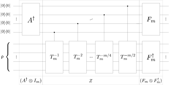
Figure 2: Circuit for the implementation of the POVM with respect to the Weyl-Heisenberg group and the vector $|\Psi\rangle=(v_{1},\ldots,v_{m})^{T}$. The vector $|\Psi\rangle$ determines the matrix $A^{\dagger}$.

For $m=2^{k}$ the circuit contains the $k$ controlled operations

$$T_{m}^{-1},T_{m}^{-2},\ldots,T_{m}^{-m/4},T_{m}^{-m/2}$$

for the implementation of the matrix $Z$. The matrix $T_{m}={\rm diag}(1,\omega,\omega^{2},\ldots,\omega^{m-1})$ can be written as Kronecker product

$$T_{m}=\left(\begin{array}[]{cc}1&0\\ 0&\omega^{m/2}\end{array}\right)\otimes\left(\begin{array}[]{cc}1&0\\ 0&\omega^{m/4}\end{array}\right)\otimes\ldots\otimes\left(\begin{array}[]{cc}1&0\\ 0&\omega\end{array}\right)\in{\cal U}(m).$$

Therefore, the matrices $T_{m}^{j}$ of the circuit in Figure 2 can be implemented efficiently on a register of qubits.

The circuit in Figure 2 is efficient if the matrix $A$ that contains the vector (3) as first row can be implemented efficiently. We can find such a matrix for the POVM with the vector

$$|\Psi\rangle=\frac{1}{\sqrt{\kappa}}(1,\alpha,\alpha^{2},\ldots,\alpha^{m/2-2},\alpha^{m/2-1},\alpha^{m/2-1},\alpha^{m/2-2},\ldots,\alpha^{2},\alpha,1)^{T}\in{\mathbb{C}}^{m}$$ (4)

where we have $\alpha\in{\mathbb{C}}$ and the normalization $\kappa=2m(1+|\alpha|^{2}+|\alpha|^{4}+\ldots+|\alpha|^{m-2})$. A matrix $A\in{\cal U}(m)$ that contains the vector (3) as first row is given by

$$A=J_{m/2}^{\dagger}\left(B_{m/4}\otimes B_{m/8}\otimes\ldots\otimes B_{4}\otimes B_{2}\otimes B_{1}\otimes B_{0}\right)J_{m/2}F_{m}^{\dagger}$$

where we use the unitary matrices

$$B_{j}=\frac{1}{\sqrt{1+|\alpha|^{2j}}}\left(\begin{array}[]{cc}1&\alpha^{j}\\ {\overline{\alpha}}^{j}&-1\end{array}\right)\in{\cal U}(2)\,.$$

Here $J_{k}$ is defined to be the permutation matrix which maps $2i\mapsto i$ and $(2i-1)\mapsto-i$ for $i=0,\ldots,k$. In our example with $m=4$ we have the matrix

$$J_{2}^{\dagger}\left(B_{1}\otimes B_{0}\right)J_{2}=\frac{1}{\sqrt{2+2|\alpha|^{2}}}\left(\begin{array}[]{cccc}1&\alpha&\alpha&1\\ {\overline{\alpha}}&-1&-1&{\overline{\alpha}}\\ {\overline{\alpha}}&-1&1&-{\overline{\alpha}}\\ 1&\alpha&-\alpha&-1\end{array}\right).$$

The circuit scheme for the implementation of the matrix

$$A^{\dagger}=F_{m}J_{m/2}^{\dagger}\left(B_{m/4}^{\dagger}\otimes B_{m/8}^{\dagger}\otimes\ldots\otimes B_{4}^{\dagger}\otimes B_{2}^{\dagger}\otimes B_{1}^{\dagger}\otimes B_{0}^{\dagger}\right)J_{m/2}$$

is shown in Figure 3.

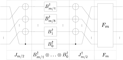
Figure 3: Implementation of the matrix $A^{\dagger}$ where $A$ is a matrix that contains the vector (3) as first row. This matrix is part of the circuit in Figure 2 for the vectors (4).

7 Conclusions and outlook

We have shown that a group-covariant POVM can be reduced to an orthogonal measurements by a unitary transform which is symmetric in the sense that it intertwines two different group representations. The symmetry of the unitary transform can be used to derive decompositions which in several cases of interest (as the Heisenberg-Weyl group) leads to an efficient quantum circuit for the implementation of the POVM.

We have argued that POVMs are often necessary in order to understand why large quantum systems show typically classical behavior on the phenomenological level. The POVM with Heisenberg-Weyl symmetry as well as the example in [5] show that the POVMs which appear in this context are often covariant with respect to some group.

Besides the physical motivation to study implementations of POVMs by means of orthogonal measurements in terms of quantum circuits there is also a motivation from computer science. The so-called hidden subgroup problem [36] is an attractive generalization of the quantum algorithms for discrete logarithms and factoring [37]. The standard approach for the hidden subgroup problem consists in a Fourier transform for the respective group followed by a suitable post-processing on the Fourier coefficients [38]. For abelian groups this post-processing consists simply in an orthogonal measurement in the computational basis. However, for non-abelian group measurements which are in fact POVMs are often more advantageous, see e. g. [39]. The POVMs which appear to be useful to solve hidden subgroup problems for non-abelian groups are naturally group-covariant. The methods presented in this paper might be useful to find quantum algorithms for the hidden subgroup problem for new classes of non-abelian groups.

References

- [1] A. S. Holevo. Probabilistic and Statistical Aspects of Quantum Theory. North Holland, Amsterdam, 1982.
- [2] C. W. Helstrom. Quantum Detection and Estimation Theory. Academic Press, New York, 1976.
- [3] Y. C. Eldar and Jr. Forney, G. D. On quantum detection and the square-root measurement. IEEE Transactions on Information Theory, 47(3):858–872, 2001.
- [4] M. Sasaki, S. M. Barnett, R. Jozsa, M. Osaki, and O. Hirota. Accessible information and optimal strategies for real symmetrical quantum sources. Phys Rev A, 59(5):3325–3335, 1999.
- [5] G. D’Ariano, P. Lo Presti, and M. Sacchi. A quantum measurement of the spin direction. Phys. Lett. A., 292(233), 2002. quant-ph/010065.
- [6] D. Giulini, E. Joos, C. Kiefer, J. Kupsch, I.-O. Stamatescu, and H. D. Zeh. Decoherence and the Appearance of a Classical World in Quantum Theory. Springer, Berlin, 1996.
- [7] P. K. Aravind. The generalized Kochen-Specker theorem. Phys. Rev. A, 68:052104, 2003.
- [8] A. Cabello. Kochen-Specker theorem for a single qubit using positive operator-valued measures. Phys. Rev. Lett., 90:190401, 2003. See also LANL preprint quant–ph/0210082.
- [9] C. A. Fuchs. Quantum Mechanics as Quantum Information (and only a little more). LANL preprint quant–ph/0205039.
- [10] A. Peres. Neumark’s theorem and quantum inseparability. Foundations of Physics, 12:1441–1453, 1990.
- [11] A. Peres. Quantum Theory: Concepts and Methods. Kluwer Academic Publishers, 1993.
- [12] A. Barenco, C. H. Bennett, R. Cleve, D. P. DiVincenzo, N. Margolus, P. Shor, T. Sleator, J. A. Smolin, and H. Weinfurter. Elementary gates for quantum computation. Physical Review A, 52(5):3457–3467, November 1995.
- [13] J. M. Myers and H. E. Brandt. Converting a positive operator-valued measure to a design for a measuring instrument on the laboratory bench. Measurement science & technology, 8:1222–1227, 1997.
- [14] Th. Decker, D. Janzing, and Th. Beth. Quantum circuits for single-qubit measurements corresponding to platonic solids. LANL preprint quant–ph/0308098. To appear in Int. Journ. Quant. Inf.
- [15] E. B. Davies. Information and quantum measurement. IEEE Transactions on Information Theory, 24(5):596–599, 1978.
- [16] G. M. D’Ariano, P. Perinotti, and M. F. Sacchi. Informationally complete measurements and groups representation. J. Opt. B: Quantum Semiclass. Opt., 6:S487–S491, 2004. See also LANL preprint quant–ph/0310013.
- [17] G. M. D’Ariano. Extremal covariant Quantum Operations and POVMs. LANL preprint quant–ph/0310024.
- [18] J. M. Renes, R. Blume-Kohout, A. J. Scott, and C. M. Caves. Symmetric informationally complete quantum measurements. Journal of Mathematical Physics, 45(6):2171–2180, 2004.
- [19] E. B. Davies. Quantum theory of open systems. Academic Press, 1976.
- [20] J. Vartiainen, M. Mottonen, and M. Salomaa. Efficient decomposition of quantum gates. Phys. Rev. Lett., 92 (17), p. 177902, 2004.
- [21] B. Huppert. Endliche Gruppen, volume I. Springer Verlag, zweiter Nachdruck der ersten Auflage, 1983.
- [22] I. M. Isaacs. Character Theory of Finite Groups. Pure and Applied Mathematics. Academic Press, 1976.
- [23] S. Egner and M. Püschel. Symmetry-Based Matrix Factorization. Journal of Symbolic Computation, 37(2):157–186, 2004.
- [24] S. Egner and M. Püschel. Automatic Generation of Fast Discrete Signal Transforms. IEEE Trans. on Signal Processing, 49(9):1992–2002, 2001.
- [25] W. C. Curtis and I. Reiner. Representation Theory of Finite Groups and Algebras. Wiley and Sons, 1962.
- [26] Th. Beth. On the computational complexity of the general discrete Fourier transform. Theoretical Computer Science, 51:331–339, 1987.
- [27] M. Clausen and U. Baum. Fast Fourier Transforms. BI-Verlag, 1993.
- [28] R. Beals. Quantum computation of Fourier transforms over the symmetric groups. In Proceedings of the Symposium on Theory of Computing (STOC), El Paso, Texas, 1997.
- [29] M. Püschel, M. Rötteler, and Th. Beth. Fast quantum Fourier transforms for a class of non-abelian groups. In Proceedings Applied Algebra, Algebraic Algorithms and Error-Correcting Codes (AAECC-13), volume 1719 of Lecture Notes in Computer Science, pages 148–159. Springer, 1999.
- [30] C. Moore, D. Rockmore, and A. Russell. Generic Quantum Fourier Transforms. In Proceedings of the Fifteenth Annual ACM-SIAM Symposium on Discrete Algorithms (SODA 2004), pages 778–787, 2004. See also LANL preprint quant–ph/0304064.
- [31] D. Coppersmith. An approximate Fourier transform useful for quantum factoring. Technical Report RC 19642, IBM Research Division, 1994.
- [32] M. Nielsen and I. Chuang. Quantum Computation and Quantum Information. Cambridge University Press, 2000.
- [33] N. Jacobson. Basic Algebra II. Freeman and Company, 1989.
- [34] A. Terras. Fourier Analysis on Finite Groups and Applications, volume 43 of Student Texts. London Mathematical Society, 1999.
- [35] J. Ziman. Principles of the Theory of Solids. Cambridge University Press, 1972.
- [36] G. Brassard and P. Høyer. An exact polynomial–time algorithm for Simon’s problem. In Proceedings of Fifth Israeli Symposium on Theory of Computing and Systems, pages 12–33. ISTCS, IEEE Computer Society Press, 1997. LANL preprint quant–ph/9704027.
- [37] P. Shor. Polynomial-time algorithms for prime factorization and discrete logarithms on a quantum computer. SIAM Journal on Computing, 26:1484–1509, 1997.
- [38] S. Hallgren, A. Russell, and A. Ta-Shma. The Hidden Subgroup Problem and Quantum Computation Using Group Representations. SIAM Journal on Computing, 32(4):916–934, 2003.
- [39] C. Moore, D. Rockmore, A. Russell, and L. J. Schulman. The power of basis selection in Fourier sampling: hidden subgroup problems in affine groups. In Proceedings of the Fifteenth Annual ACM-SIAM Symposium on Discrete Algorithms (SODA 2004), pages 1113–1122, 2004. See also LANL preprint quant–ph/0211124.