High efficiency transfer of quantum information and multi-particle entanglement generation in translation invariant quantum chains.

Abstract

We demonstrate that a translation invariant chain of interacting quantum systems can be used for high efficiency transfer of quantum entanglement and the generation of multi-particle entanglement over large distances and between arbitrary sites without the requirement of precise spatial or temporal control. The scheme is largely insensitive to disorder and random coupling strengths in the chain. We discuss harmonic oscillator systems both in the case of arbitrary Gaussian states and in situations when at most one excitation is in the system. The latter case which we prove to be equivalent to an xy-spin chain may be used to generate genuine multi particle entanglement. Such a ’quantum data bus’ may prove useful in future solid state architectures for quantum information processing.

The realization of quantum communication and computation requires at various stages the mapping between stationary and flying qubits and the subsequent transfer of quantum information between different units of our quantum information processing devices. Traditionally the stationary forms of qubits are massive systems such as atoms, ions, quantum dots or Josephson junctions while the flying qubit is a photon, ie radiation. Photons might be optimal when considering long distance communication where they may travel through free space or optical fibres. In very small quantum information processing devices such as condensed matter systems however, this is difficult as the length scale both of the component parts and their separation will generally be below optical wavelengths. In this situation, it is worth considering novel approaches for the communication of quantum information and the generation of entanglement. To this end it is of interest to consider the properties of interacting quantum systems and here in particular those of harmonic systems that are realized in various condensed matter physics settings such as nano-mechanical oscillators. While static harmonic (or spin) systems near their ground state do not exhibit long distance entanglement Audenaert EPW 02 , the situation changes drastically when considering time-dependent properties of interacting quantum systems Khaneja G 02 . Indeed, solid state devices such as arrays of nano-mechanical oscillators, described as interacting harmonic oscillators, allow for the generation Eisert PBH 03 , transfer and manipulation of entanglement Plenio HE 04 with a minimum of spatial and temporal control. However, in translation invariant systems the efficiency for this transfer decreased with distance. This can be overcome either by making the coupling strengths between neighboring systems position dependent Christandl DEL 03 ; Plenio HE 04 or by active steps such as quantum repeater stages Osborne L 03 or conclusive transfer Burgarth B 04 . Nevertheless, active steps or the fabrication of precisely manufactured spatially dependent couplings are difficult in practice and will require a significant degree of control. Furthermore, the precise value of the coupling parameters and the timing of the operations will depend on the distance across which one aims to transfer quantum information. Consequently, it would be desirable to achieve high efficiency transmission of quantum information between arbitrary places and distances with minimal spatial and temporal control. In the following we show that this is indeed possible employing translation invariant chains of interacting quantum systems with stationary couplings.

We first describe the system, termed quantum data bus, and demonstrate its functionality by numerical examples. Then we present an approximate analytical model that reveals the basic physical mechanism that is utilized in the operation of the quantum data bus. This model then allows us maximize entanglement transfer efficiency and transmission speed of the quantum data bus by adjusting the eigenfrequencies of the sender and receiver system. It also explains why the transmission is largely insensitive to disorder and random coupling strengths in the ring. We discuss the scaling behavior of the time that is required for the transfer between distant sites at a given efficiency. Finally, we show that in the regime where at most one excitation is in the system, a quantum data bus made of interacting harmonic oscillators becomes equivalent to an interacting spin chain. A further application for such a chain is the generation of three or multi-particle entangled states as we also show in this paper.

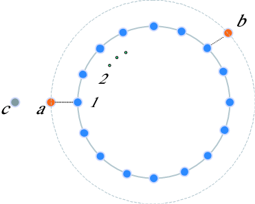
Figure 1: A ring of interacting quantum systems (blue circles) forms the quantum data bus. Two further quantum systems $a$ and $b$ (red) may couple weakly at arbitrary positions to the ring. The subsequent time evolution will allow for the transfer of quantum information or entanglement that exists between systems $a$ and the decoupled system $c$ from system $a$ to system $b$. System $c$ is decoupled but might be entangled with $a$ to study transfer of entanglement.

The model we have in mind is depicted in Fig. 1. A ring of interacting quantum systems (blue circles) forms the quantum data bus. At arbitrary positions on the ring two further quantum systems (red) may be coupled weakly to the ring. The subsequent time evolution will allow for high efficiency transfer of entanglement between the two distinguished quantum systems. The following ideas are not restricted to the specific ring like geometry presented here. The depicted geometry has been chosen because it simplifies the analytical treatment of the problem.

So far we have not specified any particular type of quantum systems nor their mutual interaction. In the following we will consider as an example the case of coupled harmonic oscillators which may be realized in various solid state settings Eisert PBH 03 . Towards the end of this article we will also consider a setting which is equivalent to a spin chain with an xy-interaction. Let us assume that the ring consists of $M$ harmonically coupled identical oscillators. We set $\hbar=\omega=m=1$ and denote the coupling strength in the ring by $c$. We assume that oscillator $a$ ($b$) couples to oscillator $1$ ($k$) with strength $\epsilon$ so that the Hamilton operator of this system including the oscillators $a,b$ and $c$ is given by

$$H(\epsilon) = \frac{1}{2}\left[\sum_{k=1}^{M}p_{k}^{2}+\sum_{k,l=1}^{M}x_{k}V_{kl}x_{l}+\sum_{i=a,b,c}(x_{i}^{2}+p_{i}^{2})\right]$$ (1)

$$+\frac{\epsilon}{2}\left[(x_{a}-x_{1})^{2}+(x_{b}-x_{k})^{2}\right]$$

with the potential matrix $V$ given by $V_{kk}=1+2c$ and $V_{k,k+1}=V_{k+1,k}=-c$ and $V_{1M}=V_{M1}=-c$ for all $k$ and zero otherwise.

In the following we will demonstrate that it is indeed possible to transmit quantum information through this system with high efficiency but minimal spatial and temporal control. For the moment we are focussing on Gaussian states, i.e., states whose characteristic function or Wigner function is Gaussian. The characteristic function determines the quantum state and as any Gaussian is determined by its first an second moments the same applies to the corresponding quantum state Eisert P 03 . In the present setting the first moments will not be directly relevant (they correspond to biases that can be removed by redefining the coordinate origin). Therefore the state of the system is determined by second moments that can be arranged in the symmetric $2N\times 2N$-covariance matrix $\Gamma_{R,S}=2\text{Re}\langle(R-\langle R\rangle)(S-\langle S\rangle)\rangle,$ where $R$ and $S$ stand for the canonical operators $x_{1},\ldots,x_{n}$ and $p_{1},\ldots,p_{n}$.

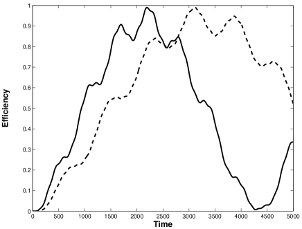
Figure 2: The efficiency of entanglement transfer, defined as ratio of transmitted entanglement to initial entanglement, between the oscillator $a$ and $b$ at opposite ends of a quantum data bus consisting of $20$ oscillators and a nearest neighbor coupling strength of $c=1$. The coupling strength of the oscillators $a$ and $b$ to the quantum data bus is $\epsilon=0.015$ (dashed line) and $\epsilon=0.021$ (solid line), The speed of propagation is proportional to the coupling strength $\epsilon$ and in both cases we observe maximal efficiency exceeding $0.99$.

Employing the Hamilton operator eq. (1) we can now study numerically the quality of the entanglement transfer between oscillators $a$ and $b$. Let us consider the situation where the harmonic oscillator $a$ and $c$ are initially in a pure entangled two-mode squeezed state

$$|\psi\rangle=\sqrt{1-q^{2}}\sum_{n=1}^{\infty}q^{n}|n\rangle|n\rangle$$ (2)

with $q=\tanh\frac{r}{2}$ which possesses the covariance matrix

$$\Gamma_{x_{a}x_{c}p_{a}p_{c}}=\frac{1}{2}\left(\begin{array}[]{cccc}\cosh r&0&-\sinh r&0\\ 0&\cosh r&0&\sinh r\\ -\sinh r&0&\cosh r&0\\ 0&\sinh r&0&\cosh r\end{array}\right)\,.$$ (7)

The entanglement as quantified by the logarithmic negativity Logneg of this state is then given by $E_{N}(|\psi\rangle)=2r$. The time evolution of the entanglement between the oscillator $a$ and $b$ at opposite ends of a quantum data bus consisting of $20$ oscillators and a nearest neighbor coupling strength of $c=1$ is given in Fig. 2. The propagation speed is proportional to $\epsilon$ and the efficiency of entanglement transfer decreases weakly with increasing speed. In both cases we find a maximal efficiency, defined as the ratio of transmitted entanglement to initial entanglement, exceeding $0.99$. It should be noted that the time required for the transfer of entanglement is independent of the distance of places where the oscillators $a$ and $b$ couple to the ring. The high quality of the entanglement transfer and its independence on the position of sender and receiver will be successfully explained by the following model that encapsulates the essential physics in the system.

We first observe that the unitary matrix $\Omega$ with matrix elements

$$\Omega_{kl}=\frac{1}{\sqrt{M}}e^{\frac{2\pi ikl}{M}}$$ (8)

achieves $V=\Omega^{\dagger}\Lambda^{2}\Omega$ with a diagonal matrix $\Lambda$ such that

$$\Lambda_{kk}^{2}=1+2c-2c\,cos\frac{2\pi k}{M}.$$ (9)

Then we can define the normal mode variables

$$X_{k} = \sum_{l=1}^{M}\Omega_{kl}x_{l},\;\;\;P_{k}=\sum_{l=1}^{M}\Omega_{kl}^{*}p_{l}$$ (10)

which ensure that $[X_{k},P_{l}]=[x_{k},p_{l}]=i\delta_{kl}$, ie the canonical commutation relations are preserved. Note that we will use the convention $X_{0}\equiv X_{M}$ and $P_{0}\equiv P_{M}$ which reflects the periodic boundary conditions of the quantum data bus. Further denote $X_{a,b,c}=x_{a,b,c}$ and $P_{a,b,c}=p_{a,b,c}$ to make the notation more uniform. In these normal modes we can write the Hamiltonian eq. (1) as

$$H(\epsilon) = \frac{1}{2}\left[\sum_{k=1}^{M}P^{\dagger}_{k}P_{k}+\Lambda_{kk}^{2}X_{k}^{\dagger}X_{k}+\sum_{i=a,b}P_{i}^{2}+(1+\epsilon)X_{i}^{2}\right]$$

$$+\frac{1}{2}(X_{c}^{2}+P_{c}^{2})-\epsilon X_{a}\sum_{l=1}^{M}\Omega_{1l}^{*}X_{l}-\epsilon X_{b}\sum_{l=1}^{M}\Omega_{kl}^{*}X_{l}$$

$$+\frac{\epsilon}{2}\sum_{lm}(\Omega_{l1}^{*}\Omega_{m1}^{*}+\Omega_{lk}^{*}\Omega_{mk}^{*})X_{l}X_{m}\,.$$

Defining the annihilation operators

$$A_{k}=\frac{\Lambda_{kk}X_{k}+iP_{k}^{\dagger}}{\sqrt{2\Lambda_{kk}}} A_{a,b,c}=\frac{X_{a,b,c}+iP_{a,b,c}}{\sqrt{2}}$$

we can rewrite the Hamilton operator in terms of the $A_{k}$. Indeed, shifting the zero of energy and moving to an interaction picture with respect to

$$H=\frac{1}{2}\sum_{k=1}^{M}P^{\dagger}_{k}P_{k}+\Lambda_{kk}^{2}X_{k}^{\dagger}X_{k}+\frac{1}{2}\sum_{i=a,b,c}P_{i}^{2}+X_{i}^{2}$$

we find

$$H_{I} = \frac{\epsilon}{2}A_{a}^{\dagger}A_{a}+\frac{\epsilon}{2}A_{b}^{\dagger}A_{b}-\epsilon\sum_{l=1}^{M}\frac{\Omega_{1l}^{*}(A_{a}e^{-it}+A_{a}^{\dagger}e^{it})+\Omega_{kl}^{*}(A_{b}e^{-it}+A_{b}^{\dagger}e^{it})}{2\sqrt{\Lambda_{ll}}}(A_{l}e^{-i\Lambda_{ll}t}+A_{M-l}^{\dagger}e^{i\Lambda_{ll}t})$$ (11)

$$+ \sum_{lm=1}^{M}\frac{\epsilon(\Omega_{l1}^{*}\Omega_{m1}^{*}+\Omega_{lk}^{*}\Omega_{mk}^{*})(A_{l}e^{-i\Lambda_{ll}t}+A_{M-l}^{\dagger}e^{i\Lambda_{ll}t})(A_{m}e^{-i\Lambda_{mm}t}+A_{M-m}^{\dagger}e^{i\Lambda_{mm}t})}{2\sqrt{\Lambda_{ll}\Lambda_{mm}}}\,.$$

In this interaction picture we find for $\epsilon=0$ that $A^{I}_{k}(t)=A^{I}_{k}(0)$ while for finite $\epsilon$ we have $\frac{d}{dt}A^{I}_{k}(t)=i[H_{I},A^{I}_{k}(t)].$ In time dependent perturbation theory using

$$\frac{A^{I}_{k}(t+\Delta t)-A^{I}_{k}(t)}{\Delta t} \cong \frac{i}{\Delta t}\int_{t}^{t+\Delta t}ds_{1}[H_{I}(s_{1}),A^{I}_{k}(t)]$$

and setting $\frac{1}{c}\ll\Delta t\ll\frac{1}{\epsilon}$ we find that to first order in $\epsilon$ the modes described by $A_{a}$ and $A_{b}$ are only coupled to one collective mode, namely the center of mass mode, described by $A_{M}$. Therefore we can ignore the contributions from all other eigenmodes. Shifting the zero of energy again we finally obtain the simplified set of equations

$$H_{approx} = \frac{\epsilon}{2}A_{a}^{\dagger}A_{a}+\frac{\epsilon}{2}A_{b}^{\dagger}A_{b}+\frac{2\epsilon}{M}A_{M}^{\dagger}A_{M}$$ (12)

$$\!\!\!\!\!\!-\frac{\epsilon}{2\sqrt{M}}[(A_{a}+A_{b})A_{M}^{\dagger}+(A_{a}^{\dagger}+A_{b}^{\dagger})A_{M}].$$

Now we write this Hamiltonian again in the quadrature components. Defining $P\equiv(P_{c},P_{a},P_{b},P_{M})^{T}$ and $X\equiv(X_{c},X_{a},X_{b},X_{M})^{T}$ we find

$$H_{approx} = P^{T}VP+X^{T}VX$$

where

$$V=\frac{1}{2}\left(\begin{array}[]{cccc}0&0&0&0\\ 0&\frac{\epsilon}{2}&0&-\frac{\epsilon}{2\sqrt{M}}\\[2.84544pt] 0&0&\frac{\epsilon}{2}&-\frac{\epsilon}{2\sqrt{M}}\\[2.84544pt] 0&-\frac{\epsilon}{2\sqrt{M}}&-\frac{\epsilon}{2\sqrt{M}}&\frac{2\epsilon}{M}\end{array}\right).$$

The above set of approximate equations of motion can be understood intuitively by a simple mechanical model. Indeed they describe the motion of a very heavy central pendulum (corresponding to the oscillators in the quantum data bus) that is coupled weakly to two comparatively light oscillators. From undergraduate mechanics we know that if one of the light pendulum is originally oscillating then, after some time, it will have stopped oscillating, while the other light pendulum is now oscillating with almost the same amplitude while the heavy central pendulum remains essentially at rest. From this simple mechanical picture the dynamics in the quantum setting that is described below can be understood quite intuitively.

That the above approximate Hamiltonian represents a good approximation to the true dynamics can be seen from a comparison of the exact time evolution with that generated by the approximate Hamiltonian. In figure 3 we chose a ring with $20$ oscillators, $c=10$ and $\epsilon=0.021$. The observable mismatch of between the frequencies is due to second order corrections to the approximate model. Furthermore, as the excitation of a quantum in the center of mass mode corresponds to the simultaneous in-phase motion of all the oscillators in the quantum data bus and the fact that the oscillators $a$ and $b$ couple predominantly to the center of mass mode $M$ also explains why the entanglement transfer is distance independent. The frequency of the center-of-mass mode is independent of both the coupling strengths between oscillators in the chain and possible disorder in which oscillators are coupled as long as there is a connected path of coupled oscillators between $a$ and $b$. Therefore the transmission of quantum information between $a$ and $b$ will depend only weakly on disorder and randomness. The main correction arises when the frequency separation between the lowest two eigen-modes becomes small so that off-resonant couplings of the oscillators $a$ and $b$ to modes other than the center-of-mass mode become non-negligible.

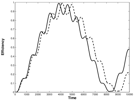
Figure 3: Comparison of the approximation and the exact time evolution for a ring of $20$ oscillators with $c=10$ and $\epsilon=0.021$. The dotted line is the approximation and the solid line is exact.

In the derivation of eq. (12) we have neglected many terms that led to oscillating contributions in the Hamiltonian. These neglected terms will lead to corrections whose size will depend on the length $M$ of the quantum data bus and will affect both, the speed of propagation but also its efficiency. As we can always adjust the waiting time, corrections to the propagation speed are less relevant. An efficiency reduction due to population losses is more serious as it will require the application of error correction methods. For the setting described by the Hamiltonian eq. (1) we will now present an estimate the size of these corrections. Indeed, following eq. (11) we neglect all terms that couple the modes $a$ and $b$ non-resonantly to eigenmodes different than the center of mass mode. For small coupling strength $\epsilon$ the rapid oscillations will reduce the population in these modes significantly. The mode, other than the center of mass mode, with the smallest oscillation frequency will be the mode $M-1$. For large $M$ the frequency difference to the center of mass mode is given by $\Delta=2\pi^{2}c/M^{2}$ and the coupling strength to this mode is of the order of $\epsilon/2\sqrt{M}$. The loss of population into this mode, which is of order $\left(\frac{\epsilon\sqrt{M}}{2}\right)^{2}\left(\frac{4\pi^{2}c}{M^{2}}\right)^{-2}$, should be small, ie

$$\frac{\epsilon}{c}\ll\frac{4\pi^{2}}{M^{3/2}}\,.$$ (13)

From eq. (12) we determine that the speed of propagation is proportional to $\epsilon/(2M)$. For a prescribed transfer efficiency the transmission time therefore scales as

$$T\sim\frac{2M}{\epsilon}\sim\frac{M^{5/2}}{2\pi^{2}c}\,.$$ (14)

The error source that enters this scaling is the population loss to off-resonant modes. This suggest that this scaling can be improved considerably when one allows for a fixed frequency difference of the oscillators $a$ and $b$ compared to the oscillators in the quantum data bus such that the oscillators $a$ and $b$ become resonant with a different collective mode whose frequency difference to the neighboring modes is as large as possible. Indeed, if we couple $a$ and $b$ to the mode described by $A_{M/4}$, ie if we shift the eigenfrequencies of $a$ and $b$ by $2c$, then we find that the next mode is separated by a frequency difference $\Delta=2c\pi/M$ and the couplings strength to this neighbouring mode is again of the order of $\epsilon/2\sqrt{M}$. As a consequence the population loss to other modes is of the order of $(\epsilon\sqrt{M}/(4\pi c))^{2}$ and we only need to ensure that

$$\frac{\epsilon}{c}\ll\frac{4\pi}{\sqrt{M}}$$ (15)

so that the propagation time for fixed transfer efficiency scales as

$$T\sim\frac{2M}{\epsilon}\sim\frac{M^{3/2}}{2\pi c}\,.$$ (16)

This improved scaling has been achieved by coupling the oscillators $a$ and $b$, but it should be noted that unlike the center of mass mode $M$ this mode will have nodes. As a consequence there will be relative positions of oscillator $a$ and $b$ such that they will not couple, namely, when one is sitting at a node while the other is at an anti-node. Indeed, the $M/4$ mode has a node at every second oscillator of the ring, so that the oscillators $a$ and $b$ couple only when their distance is an even number of oscillators.

Finally we demonstrate that the above considerations are not restricted to the continuous variable regime and the properties of Gaussian continuous variable states. Indeed, we can equally well consider a situation in which we restrict our dynamics to the subspace spanned by the the vacuum and those states that corresponds to a single excitation. The derivation of the approximate model starting from Hamiltonian eq. (1) remains of course valid. In the basis represented by the states $\{|00\rangle_{ab}|0\rangle_{M},|10\rangle_{ab}|0\rangle_{M},|01\rangle_{ab}|0\rangle_{M},|00\rangle_{ab}|1\rangle_{M}\}$ where $|1\rangle_{M}\equiv\frac{1}{\sqrt{M}}\sum_{r=1}^{M}a_{r}^{\dagger}|vacuum\rangle$ we can rewrite the Hamiltonian eq. (12) as

$$H_{approx} = \frac{1}{2}\left(\frac{2\epsilon}{M}-\frac{\epsilon}{2}\right)({\sf 1\rule{0.43057pt}{6.54443pt}\rule[-0.04303pt]{1.29167pt}{0.43057pt}}+\sigma_{z}^{M})$$

$$-\frac{\epsilon}{4\sqrt{M}}[(\sigma_{x}^{a}+\sigma_{x}^{b})\sigma_{x}^{M}+(\sigma_{y}^{a}+\sigma_{y}^{b})\sigma_{y}^{M}]$$

which corresponds to a spin chain with an xy-interaction Alves CJ under the same constraint of considering at most a single excitation. This similarity between a harmonic oscillator systems and a spin chain is not due to the approximations in the derivation of eq. (12) but a generic feature when one limits the number of excitations to at most one. A simple computation shows that generally a harmonic chain in the rotating wave-approximation and the single excitation regime will be equivalent to a spin chain with xy-interaction in the same regime.

Continuing in this setting of a spin chain we now demonstrate that multi-particle entanglement multiparticle can be generated with a quantum data bus extending the ideas employed in the paper so far. While we focus on the discrete case, i.e. the spin Hamiltonian, one may carry out a similar investigation for the harmonic oscillator case. For the purpose of the generation of entangled states there is no need of including the decoupled oscillator in the discussion. While the ideas presented below may easily be generalized to many oscillators let us, for simplicity, consider three oscillators coupled to the chain. We assume that the oscillator $a$ ($b$, $c$) couples to oscillator $1$ ($k_{1}$, $k_{2}$) of the quantum data bus with strength $\epsilon$ so that the Hamilton operator of this system is a generalization of eq. (High efficiency transfer of quantum information and multi-particle entanglement generation in translation invariant quantum chains.) and is given by

$$H = \frac{1}{2}\left(\frac{3\epsilon}{M}-\frac{\epsilon}{2}\right)({\sf 1\rule{0.43057pt}{6.54443pt}\rule[-0.04303pt]{1.29167pt}{0.43057pt}}+\sigma_{z}^{M})$$

$$-\frac{\epsilon}{4\sqrt{M}}[(\sigma_{x}^{a}+\sigma_{x}^{b}+\sigma_{x}^{c})\sigma_{x}^{M}+(\sigma_{y}^{a}+\sigma_{y}^{b}+\sigma_{y}^{c})\sigma_{y}^{M}].$$

Let us now suppose that the initial state of the system is

$$|\psi(0)\rangle=|1\rangle_{a}|0\rangle_{b}|0\rangle_{c}|0\rangle_{M}\equiv|1000\rangle$$ (19)

where a single excitation is initially present in oscillator $a$. The evolved state according to the Hamiltonian eq. (High efficiency transfer of quantum information and multi-particle entanglement generation in translation invariant quantum chains.) may then be written as

$$|\psi(t)\rangle=a(t)|0001\rangle+b(t)|1000\rangle+c(t)|0100\rangle+d(t)|0010\rangle$$ (20)

where, with the scaled time $\tau\equiv\frac{\epsilon\,t}{2}$ and the constant $\alpha\equiv\frac{3-M}{M}$, as well as

$$C(M,\tau) = \cos(\sqrt{\frac{12+\alpha^{2}}{M}}\;\tau/2)$$

$$S(M,\tau) = \sin(\sqrt{\frac{12+\alpha^{2}}{M}}\;\tau/2)$$ (21)

the time dependent coefficients are given by

$$a(\tau) = i\frac{e^{-i\alpha\tau/2}}{\sqrt{12+M\alpha^{2}}}C(M,\tau)$$ (22)

$$b(\tau) = \frac{2}{3}+\frac{e^{-i\alpha\tau/2}}{3}\left[C(M,\tau)+i\frac{S(M,\tau)}{\sqrt{12+M\alpha^{2}}}\right]$$

$$c(\tau) = d(\tau)=-\frac{1}{3}+\frac{e^{-i\alpha\tau/2}}{3}\left[C(M,\tau)+i\frac{S(M,\tau)}{\sqrt{12+M\alpha^{2}}}\right].$$

From eq. (22) we can see that in the limit of large $M$, the coefficient $a(\tau)$ tends to zero indicating that the quantum data bus disentangles from the three oscillators and the result may be a W state of the form

$$|W_{x,y,z}\rangle\otimes|0\rangle_{M}=(x|100\rangle+y|010\rangle+z|001\rangle)\otimes|0\rangle_{M}$$ (23)

In order to see that this is the case we plot the overlap between the W state eq. (23) and the evolved state obtained with the use of eq. (20) and eq. (22). For the case of $70$ oscillators in the chain, and the W state with $x=-y=-z=1/\sqrt{3}$, it is shown in figure 4 that the overlap is about 96%. The overlap is not complete due to fact that the population of the state $|0001\rangle$ does not vanish and that the coefficients eq. (22) have a small imaginary part. It should be noted that the second of these effects can be reduced significantly by employing subsequent local unitary rotations which are irrelevant when considering entanglement properties of a state. In figure 5 we show the populations in function of the scaled time $\tau$.

Figure 4: Overlap between the W state with $x=-y=-z=1/\sqrt{3}$ and the evolved state of the system. The ring consists of $70$ oscillators.

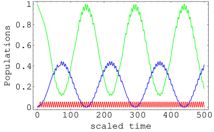
Figure 5: Time evolution of the populations, $|a(\tau)|^{2}$ in red, $|b(\tau)|^{2}$ in green, and $|c(\tau)|^{2}=|d(\tau)|^{2}$ in blue. The ring consists of $70$ oscillators.

For generating different W states one could vary the coupling constants independently what would lead to the following Hamiltonian to the system

$$H = \frac{\epsilon_{a}}{4}({\sf 1\rule{0.43057pt}{6.54443pt}\rule[-0.04303pt]{1.29167pt}{0.43057pt}}+\sigma_{z}^{a})+\frac{\epsilon_{b}}{4}({\sf 1\rule{0.43057pt}{6.54443pt}\rule[-0.04303pt]{1.29167pt}{0.43057pt}}+\sigma_{z}^{b})+\frac{\epsilon_{c}}{4}({\sf 1\rule{0.43057pt}{6.54443pt}\rule[-0.04303pt]{1.29167pt}{0.43057pt}}+\sigma_{z}^{c})$$

$$+\frac{\epsilon_{a}+\epsilon_{b}+\epsilon_{c}}{2M}({\sf 1\rule{0.43057pt}{6.54443pt}\rule[-0.04303pt]{1.29167pt}{0.43057pt}}+\sigma_{z}^{M})-\frac{\epsilon_{a}}{4\sqrt{M}}(\sigma_{x}^{a}\sigma_{x}^{M}+\sigma_{y}^{a}\sigma_{y}^{M})$$

$$-\frac{\epsilon_{b}}{4\sqrt{M}}(\sigma_{x}^{b}\sigma_{x}^{M}+\sigma_{y}^{b}\sigma_{y}^{M})-\frac{\epsilon_{c}}{4\sqrt{M}}(\sigma_{x}^{c}\sigma_{x}^{M}+\sigma_{y}^{c}\sigma_{y}^{M}).$$

In summary, we have demonstrated that it is possible to transfer quantum information with high efficiency but minimal spatial and temporal control between arbitrary sites of a translation invariant chain of quantum systems. We have shown that this process works in the continuous variable regime but also the the single excitation regime when the system becomes equivalent to the dynamics exhibited by a single excitation in a spin chain with xy-interaction. This interaction may be generalized to include more oscillators coupled to the chain allowing the generation of multi-particle entangled states. All these suggest that translation invariant chains of interacting quantum systems are promising candidates for the transport of quantum information in solid state realizations of quantum information processing devices.

We acknowledge discussions with S. Benjamin, S. Bose and A. Ekert at an IRC discussion group and J. Eisert on many occasions. This work is part of the QIP IRC (www.qipirc.org) supported by EPSRC (GR/S82176/01) and by the Brazilian Agency Fundacão de Amparo a Pesquisa do Estado de São Paulo grant no 02/02715-2, and a Royal Society Leverhulme Trust Senior Research Fellowship.

References

- (1) K. Audenaert, J. Eisert, M.B. Plenio, and R.F. Werner, Phys. Rev. A 66, 042327 (2002); M.B. Plenio, J. Eisert, J. Dreissig and M. Cramer, e-print arxiv quant-ph/0405142.
- (2) N. Khaneja and S.J. Glaser, Phys. Rev. A 66, 060301(R) (2002).
- (3) J. Eisert, M.B. Plenio, S. Bose and J. Hartley, Phys. Rev. Lett. 93, 190402 (2004).
- (4) M.B. Plenio, J. Hartley and J. Eisert, New J. Phys. 6, 36 (2004)
- (5) M. Christand, N. Datta, A. Ekert, and A.J. Landahl, Phys. Rev. Lett. 92, 187902 (2004).
- (6) T. Osborne and N. Linden, arXiv quant-ph/0312141.
- (7) D. Burgarth and S. Bose, arXiv quant-ph/0406112
- (8) J. Eisert and M.B. Plenio, Int. J. Quant. Inf. 1, 479 (2003).
- (9) J. Eisert and M.B. Plenio, J. Mod. Opt. 46, 145 (1999); J. Eisert (PhD thesis, Potsdam, February 2001); G. Vidal and R.F. Werner, Phys. Rev. A 65, 32314 (2002); K. Audenaert, M.B. Plenio, and J. Eisert, Phys. Rev. Lett. 90, 027901 (2003).
- (10) S.R. Clarke, C. Moura-Alves and D. Jaksch, quant-ph/0406150.
- (11) M. Murao, M.B. Plenio, S. Popescu, V. Vedral, and P.L. Knight, Phys. Rev. A 57, 4075 (1998); N. Linden, S. Popescu, M. Westmoreland and B. Schumacher, e-print arxiv quant-ph/9912039; M.B. Plenio and V. Vedral, J. Phys. A 34, 6997 (2001).