Arbitrarily accurate composite pulse sequences

Abstract

Systematic errors in quantum operations can be the dominating source of imperfection in achieving control over quantum systems. This problem, which has been well studied in nuclear magnetic resonance, can be addressed by replacing single operations with composite sequences of pulsed operations, which cause errors to cancel by symmetry. Remarkably, this can be achieved without knowledge of the amount of error $\epsilon$. Independent of the initial state of the system, current techniques allow the error to be reduced to $O(\epsilon^{3})$. Here, we extend the composite pulse technique to cancel errors to $O(\epsilon^{n})$, for arbitrary $n$.

Precise and complete control over closed quantum systems is a long-sought goal in atomic physics, molecular chemistry, condensed matter research, with fundamental implications for metrologyBollinger et al. (1996); Bennett and Shor (1998) and computationM.A. Nielsen and I.L. Chuang (2000); Steane (1998). Achieving this goal will require careful compensation for errors of both random and systematic nature. And while recent advances in quantum error correctionGottesman (1998); Steane (1996); Knill and Laflamme (1997) allow all such errors to be removed in principle, active error correction requires expanding the size of the quantum system, and feedback measurements which may be unavailable. Furthermore, in many systems, errors may be dominated by those of systematic nature, rather than random errors, as when the classical control apparatus is miscalibrated or suffers from inhomogeneities over the spatial extent of the target quantum system.

Of course, systematic errors can be reduced simply by calibration, but that is often impractical, especially when controlling large systems, or when the required control error magnitude is smaller than that easily measurable. Interestingly, however, systematic errors in controlling quantum systems can be compensated without specific knowledge of the magnitude of the error. This fact is loreFreeman (1997) in the art of NMR, and is achieved using the method of composite pulses, in which a single imperfect pulse with fractional error $\epsilon$ is replaced with a sequence of pulses, which reduces the error to $O(\epsilon^{n})$.

Composite pulse sequences have been constructed to correct for a wide variety of systematic errors Levitt and Freeman (1979); Tycko (1983); Freeman (1997). These include pulse amplitude, phase, and frequency errors and can be applied to any system with sufficient control. As system control increases, new uses for composite pulses emerge. A remarkable example is the recent teleporation of an atomic state in ion traps Riebe et al. (2004); Barrett et al. (2004). Barret et al. use a composite pulse for individual addressing, while Reibe et al. use a composite pulse to perform two qubit operations.

In the context of spectroscopy, the goal is often to maximize the measurable signal from a system which starts in a specific state. Thus, while composite sequences have been developedLevitt and Ernst (1983) which can reduce errors to $O(\epsilon^{n})$ for arbitrary $n$, these sequences are not general and do not apply, for example, to quantum computation, where the initial state is arbitrary, and multiple operations must be cascaded to obtain desired multi-qubit transformations.

Only a few composite pulse sequences are known which are fully compensating,Levitt (1986); Wimperis (1994) meaning that they work on any initial state and can replace a single pulse without further modification of other pulses. As has been theoretically discussedCummins and Jones (2000); Jones (2002); McHugh and Tawnley (2004) and experimentally demonstrated in ion traps Gulde et al. (2003); Riebe et al. (2004); Barrett et al. (2004) and Josephson junctions Collin et al. (2004), these sequences can be valuable for precise single and multiple-qubit control using gate voltages or laser excitation.

Previously, the best fully compensating composite pulse sequence knownWimperis (1994); Cummins and Jones (2000); Jones (2002); McHugh and Tawnley (2004) could only correct errors to $O(\epsilon^{3})$. Here, we present a new, and systematic technique for creating composite pulse sequences to correct errors to $O(\epsilon^{n})$, for arbitrary $n$. The technique presented is very general and can be used to correct a wide variety of systematic errors. Below, our technique is illustrated for the specific case of systematic amplitude errors, using two approaches. Also discussed is the number of pulses required as a function of $n$.

The problem of systematic amplitude errors is modeled by representing single qubit rotations as

$$R_{\phi}\left(\theta\right)=\exp\left[-i\frac{\theta}{2}\sigma_{\phi}\right]\,,$$ (1)

where $\theta$ is the desired rotation angle about about the axis that makes the angle $\phi$ with the $\hat{x}$-axis and lies in the $\hat{x}-\hat{y}$ plane, $\sigma_{\phi}=\cos(\phi)X+\sin(\phi)Y$, and $X$ and $Y$ are Pauli operators. $R_{\phi}\left(\theta\right)$ is the ideal operation, and due to errors, the actual operation is, instead, $M_{\phi}\left(\theta\right)=R_{\phi}\left(\theta(1+\epsilon)\right)$, where the angle of rotation differs from the desired $\theta$ by the factor $1+\epsilon$. Note that $\phi$ and $\theta$ may be specified arbitrarily, but the error $\epsilon$ is fixed for all operations, and unknown.

Two methods for constructing composite pulses. A composite pulse sequence $R_{\phi}^{[n]}\left(\theta\right)$ is a sequence of operations $\{M_{\phi}(\theta)\}$ such that $R_{\phi}^{[n]}\left(\theta\right)=R_{\phi}\left(\theta\right)+O(\epsilon^{n+1})$, for unknown error $\epsilon$. To construct $R_{\phi}^{[n]}\left(\theta\right)$, we begin with two simple observations: first, $R_{\phi}\left(-\theta\epsilon\right)M_{\phi}\left(\theta\right)=R_{\phi}\left(\theta\right)$ and second, $M_{\phi}\left(2k\pi\right)=\pm R_{\phi}\left(2k\pi\epsilon\right)$ when $k$ is an integer. A composite pulse sequence can thus be obtained by finding ways to approximate $R_{\phi}\left(-\theta\epsilon\right)$ by a product of operators $R_{\phi_{l}}\left(2k_{l}\pi\epsilon\right)$. We obtain this using two approaches.

The first approach we call the Trotter-Suzuki (TS) method. Suzuki has developed a set of Trotter formulas that when given a Hamiltonian $B$ and and a series of Hamiltonians $\{A_{l}\}$ such that $B=\sum{A_{l}}$ there exists a set of real numbers $\{p_{jn}\}$ such that

$$\exp\left(-iBt\right)=\prod_{j,l}\exp\left(-ip_{jn}A_{l}t\right)+O(t^{n+1})\,,$$ (2)

and $\sum_{j}p_{jn}=1$ Suzuki (1992). Without loss of generality, we may limit ourselves to expansions where the $p_{jn}$ are rational numbers, and assume the goal is to approximate $R_{0}\left(-\theta\epsilon\right)$. Using Eq. (2), we set $t=\epsilon$ and $B=-(\theta/2)X$. Then we choose $A_{1}=A_{3}=m\pi(X\cos\phi+Y\sin\phi)$ and $A_{2}=2m\pi(X\cos\phi-Y\sin\phi)$ where $\phi$ and $m$ fulfill the conditions that $4m\pi\cos\phi=\theta/2$ (i.e., $A_{1}+A_{2}+A_{3}=B$) and $q_{jn}=p_{jn}m$ is an integer. This yields an $n$th order correction sequence

$$F_{n} = \prod_{j}M_{\phi}\left(2\pi q_{jn}\right)M_{-\phi}\left(4\pi q_{jn}\right)M_{\phi}\left(2\pi q_{jn}\right)$$ (3)

$$= R_{0}\left(-\theta\epsilon\right)+O(\epsilon^{n+1})=R_{0}^{[n]}\left(-\theta\epsilon\right)$$

and the associated $n$th order composite pulse sequence $F_{n}M_{0}\left(\theta\right)=R_{0}^{[n]}\left(-\theta\epsilon\right)R_{0}\left(\theta\epsilon\right)R_{0}\left(\theta\right)=R_{0}^{[n]}\left(\theta\right)$, thus giving a composite pulse sequence of arbitrary accuracy.

The second approach we refer to as the Solovay-Kitaev (SK) method, as it uses elements of the proof of the Solovay-Kitaev theorem Kitaev et al. (2002). First, note that rotations $U_{k}(A)=I+A\epsilon^{k}+O(\epsilon^{k+1})$ can be constructed for arbitrary $2\times 2$ Hermitian matrices $A$, and $k\geq 1$, recursively. This is done using an observation (from Kitaev et al. (2002)) relating the commutator $[A,B]=AB-BA$ to a sequence of operations, $\exp(-iA\epsilon^{l})\exp(-iB\epsilon^{m})\exp(iA\epsilon^{l})\exp(iB\epsilon^{m})=\exp([A,B]\epsilon^{l+m})+O(\epsilon^{l+m+1})$. Thus to generate $U_{k}(A)$ it suffices to generate $U_{\lceil{k/2}\rceil}(B)$ and $U_{\lfloor{k/2}\rfloor}(C)$ such that $[B,C]=A$ (choices of integers other than $\left\lceil k/2\right\rceil$ and $\left\lfloor k/2\right\rfloor$ which sum to $k$ are also fine, but less optimal).

Next, we inductively construct a composite pulse sequence $F_{n}$ for $R_{0}\left(\theta\right)$. Note that the first order correction sequence can be written as $F_{1}=M_{\phi}\left(2\pi\right)M_{-\phi}\left(2\pi\right)=R_{0}\left(-\theta\epsilon\right)+O(\epsilon^{2})$ by selecting $4\pi\cos(\phi)=\theta$. Assume we have $F_{n}=R_{0}\left(-\theta\epsilon\right)-iA_{n+1}\epsilon^{n+1}+O(e^{n+2})$. We can then construct a sequence to correct for the next order, using $F_{n+1}=U_{n+1}(A_{n+1})F_{n}$, where $U_{n+1}(A_{n+1})$ is constructed as above. Iteratively applying this method for $k=1,\ldots,n$ yields an $n$th order composite pulse sequence, $F_{n}M_{0}\left(\theta\right)=R_{0}^{[n]}\left(\theta\right)$, for any $n$. This method, which appears to be unrelated to previous composite pulse techniquesLevitt and Ernst (1983); Freeman (1997), gives an efficient algorithm to calculate sequences for specific $\theta$ and $\phi$ but not necessarily a short analytical description of the sequence. Furthermore, the Solovay-Kitaev technique relies on general properties of Hamiltonians and can be applied without modification to other systematic error models, e.g., frequency errors.

Examples. The TS and SK techniques described above are general and apply to a wide variety of errors; explicit application of the techniques to generate $R_{0}^{[n]}\left(\theta\right)$ sequences for specific $n$ can take advantage of symmetry arguments, composition of techniques, and relax some of our assumptions to minimize both the residual error and the sequence length.

First, we explicitly write out the TS composite pulses and connect them to the well-known pulse sequences of Wimperis Wimperis (1994). We choose to use the TS formulas that are symmetric under reversal of pulses, i.e an anagram. These formulas remove all even-ordered errors by symmetry, and thus yield only even-order composite pulse sequences. For convenience, we introduce the notation $S_{1}(\phi_{1},\phi_{2},m)=M_{\phi_{1}}\left(m\pi\right)M_{\phi_{2}}\left(2m\pi\right)M_{\phi_{1}}\left(m\pi\right)$ and $S_{n}(\phi_{1},\phi_{2},m)=S_{n-1}(\phi_{1},\phi_{2},m)^{4^{n-1}}\times S_{n-1}(\phi_{1},\phi_{2},-2m)S_{n-1}(\phi_{1},\phi_{2},m)^{4^{n-1}}$. We can now define a series of $n$ order composite pulses P$n$ as

$$\mbox{P}0 = M_{0}\left(\theta\right)$$ (4)

$$\mbox{P}2 = M_{\phi_{1}}\left(2\pi\right)M_{-\phi_{1}}\left(4\pi\right)M_{\phi_{1}}\left(2\pi\right)\mbox{P}0$$ (5)

$$\mbox{P}{2j} = S_{j}(\phi_{j},-\phi_{j},2)\mbox{P}0$$ (6)

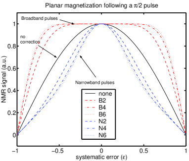
where $\phi_{j}=\cos^{-1}-\frac{\theta}{8\pi f_{j}}$ and $f_{j}=(2^{(2j-1)}-2)f_{j-1}$ when $f_{1}=1$. $\mbox{P}2$ is exactly the passband sequence PB1 described by Wimperis Wimperis (1994). Fig. 1 compares the performance of these high-order passband pulse sequences.

Wimperis also proposes a similar broadband sequence, BB1=$S_{1}(\phi_{B1},3\phi_{B1},1)\mbox{P}0$ where $\phi_{B1}=\cos^{-1}\left(-\frac{\theta}{4\pi}\right)$. The broadband sequence corrects over a wider range of $\epsilon$ by minimizing the first order commutator and thus the leading order errors. Furthermore, although BB1 and PB1 appear different when written as imperfect rotations, a transformation to true rotations shows that they have the same form,

$$\mbox{PB}1 = M_{\phi_{1}}\left(2\pi\right)M_{-\phi_{1}}\left(4\pi\right)M_{\phi_{1}}\left(2\pi\right)P0$$

$$= R_{\phi_{1}}\left(2\pi\epsilon\right)R_{-\phi_{1}}\left(4\pi\epsilon\right)R_{\phi_{1}}\left(2\pi\epsilon\right)\mbox{P}0$$

$$\mbox{BB}1 = M_{\phi_{B1}}\left(\pi\right)M_{3\phi_{B1}}\left(2\pi\right)M_{\phi_{B1}}\left(\pi\right)\mbox{P}0$$ (7)

$$= R_{\phi_{B1}}\left(\pi\epsilon\right)R_{-\phi_{B1}}\left(2\pi\epsilon\right)R_{\phi_{B1}}\left(\pi\epsilon\right)\mbox{P}0.$$ (8)

This “toggled” frame suggests a way to create higher-order broadband pulses. One simply takes a higher-order passband sequence and replaces each element $S_{1}(\phi_{j},-\phi_{j},m)$ with $S_{1}(\phi_{Bj},-\phi_{Bj}+4\phi_{Bj}(m/2\mod 2),m/2)$ where $\phi_{Bj}$ satisfies the condition $\cos(\phi_{Bj})=2\cos(\phi_{j})$. Applying this to P$n$ creates a family of broadband composite pulses, B$n$.

Similar extensions allow creation of another kind of composite pulse (useful, for example, in magnetic resonance imaging), which increase error so as to perform the desired operation for only a small window of error. Such “narrowband” pulse sequences N$n$ may be obtained starting with a passband sequence, P$n$, and dividing the angles of the corrective pulses by $2$. These higher-order narrowband pulses may be compared with the Wimperis sequence NB$1$ Wimperis (1994), as shown in Fig. 1.

Figure 1: Comparison of the narrowband and broadband composite pulse sequences generated by the TS method. The Wimperis BB1, PB1, and NB1 sequences are included in this family, and are equivalent to B2, P2, and N2.

The SK method yields a third set of $n$th order composite pulses, SK$n$, and for concreteness, we present an explicit formulation of this method. It is convenient to let $U_{nX}(a)=I-ia^{n}\frac{X}{2}\epsilon^{n}+O(\epsilon^{n+1})$, such that one can then generate $U_{nZ}(a)=M_{90}\left(-\pi/2\right)U_{nX}(a)M_{90}\left(\pi/2\right)$ and $U_{nY}(a)=M_{45}\left(\pi/2\right)U_{nX}(a)M_{45}\left(-\pi/2\right)$ . Using the first-order rotations

$$U_{1X}(a)=M_{\phi}\left(2\pi\left\lceil\frac{a}{4\pi}\right\rceil\right)M_{-\phi}\left(2\pi\left\lceil\frac{a}{4\pi}\right\rceil\right)\,,$$ (9)

where $\phi=\cos^{-1}(a/(4\pi\left\lceil\frac{a}{4\pi}\right\rceil))$, as described above, we may recursively construct $U_{nX}(a)=U_{\left\lfloor n/2\right\rfloor Y}(a)U_{\left\lceil n/2\right\rceil Z}(a)U_{\left\lfloor n/2\right\rfloor Y}(-a)U_{\left\lceil n/2\right\rceil Z}(-a)$, for any $n>1$ and any $a$.

With these definitions, the first order SK composite pulse for $R_{0}^{[n]}\left(\theta\right)$ is simply

$$\mbox{SK}1=U_{1X}(\theta)M_{0}\left(\theta\right)=R_{0}\left(\theta\right)-i\frac{A_{2}}{2}\epsilon^{2}+O(\epsilon^{3})\,.$$ (10)

From the $2\times 2$ matrix $A_{2}$, we can then calculate the norm $\|A_{2}\|$ and the planar rotation $R_{A_{2}}$ that performs $R_{A_{2}}(-A_{2})R_{A_{2}}^{-1}=\|A_{2}\|X$. The second order SK composite pulse is then

$$\mbox{SK}2 = M_{A_{2}}^{-1}U_{2X}(\|A_{2}\|^{1/2})M_{A_{2}}{\rm SK}1$$ (11)

$$= R_{0}\left(\theta\right)-i\frac{A_{3}}{2}\epsilon^{3}+O(\epsilon^{4})$$ (12)

where $M_{A_{2}}$ is the imperfect rotation corresponding to the perfect rotation $R_{A_{2}}$.

The $n$th order SK composite pulse family is thus

$$\mbox{SK}n = M_{A_{n}}^{-1}U_{nX}(\|A_{n}\|^{1/n})M_{A_{n}}\,{\rm SK}(n-1)$$ (13)

$$= R_{0}\left(\theta\right)-i\frac{A_{n+1}}{2}\epsilon^{n+1}+O(\epsilon^{n+2})\,.$$ (14)

A nice feature of the SK method is that when given a composite pulse of order $n$ described by any method one can compose a pulse of order $n+1$. The “pure” SK method SK$n$ is outperformed in terms of both error reduction and pulse number by the TS method B$n$ for $n\leq 4$. Therefore, we apply the SK method for orders $n>4$ using B$4$ as our base composite pulse. We label these pulses SB$n$.

Performance and efficiency. Two important issues with composite pulses are the actual amount of error reduction as a function of pulse error, and the time required to achieve a desired amount of error reduction. These performance metrics are shown in Fig. 2, comparing the SK, broadband, and passband composite pulses for varying error $\epsilon$, and $\phi=0$, and using as the composite pulse error $E=\|R_{\phi}\left(\theta\right)-R_{\phi}^{[n]}\left(\theta\right)\|$. We find that for practical values of error reduction, $n<30$, the number of $\pi$ pulses required to reduce error to $O(\epsilon^{n})$ grows as $\sim n^{3.09}$, which is close to the lower bound of $\sim n^{3}$ which can be analytically derivedBrown et al. (2004). In contrast, the TS sequence B$n$ requires $O(\exp(n^{2}))$ pulses.

Figure 2: Composite pulse error, $E$, as a function of base error, $\epsilon$ for a variety of composite pulse sequences. P$n$, B$n$, SK$n$ and SB$n$ are the $n$th order passband, broadband, SK, and combined B4-SK sequences, respectively. The number in the brackets refers to the number of imperfect $2\pi$ rotations in the correction sequence. Note how pulses of the same order (such as P6, B6, SK6, SB6) have the same slope (asymptotic scaling) for low values of $\epsilon$, but can have widely varying performance when $\epsilon$ is large. The inset plots the scaling of this sequence length with order $n$ for SK$n$ (SB$n$ is very similar) for $n\leq 30$ and compares it with the upper bound obtained with numerical methods.

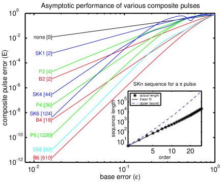
For a wide range of base errors $\epsilon$, the TS formulation out-performs the SK method in achieving a low composite pulse error, $E$. The recursive nature of the TS methods builds off elements that remove lower order errors, resulting in a rapid increase of pulse number and a monotonic decrease in effective error at every order for any value of the base error. However, the SK approach is superior to the TS method for applications requiring incredible precision, $E\leq 10^{-12}$, from relatively precise controls, $\epsilon<10^{-2}$.

The SK and TS pulse sequences presented here are conceptually simple but may not be optimal. Integrating ideas from both methods, we can develop new families of composite pulses. As an example, the SK method relies on cancellation of error order by order by building up sequences of $2\pi$ pulses. However, there is no reason that the basic unit should be a single pulse. Instead, one can build a sequence from TS (B2) style pulse triplets, $G(\phi_{1})=S_{1}(\phi_{1},3\phi_{1},1)$. By using an additional symmetry that the $\operatorname{Tr}\left(YG(-\phi_{1})G(\phi_{1})\right)=0$, the leading order error is guaranteed to be proportional to $X$ at the cost of doubling the pulse sequence. The resulting pulses are of length $\exp(n)$ (compared to $\exp(n^{2})$ for TS), broadband compared to SK sequences, and described in detail in Brown et al. (2004).

Conclusions. We have presented a set of tools that allows one to generate arbitrarily accurate composite pulse sequences for systematic, but unknown, error. As an example, we have constructed explicit composite pulse sequences for errors in rotation angle. These can be constructed with $O(n^{3})$ pulses, for $n\lesssim 30$. For high-precision applications such as quantum computation, these pulses allow one to perform accurate operations even with large errors. Practically, the B4 and B2=BB1 pulse sequences seem most useful, depending on the magnitude of error.

While we have focused on composite pulse sequences for rotation errors, we emphasize that these methods also apply to correcting systematic errors in control phase and frequencyBrown et al. (2004). For example, a frequency error can be represented for an expected rotation $R_{0}(\theta)$ as $M^{\prime}_{0}(\theta)=\exp\left(-i(\theta/2X+|\theta/2|\delta Z)\right).$ Note that $M^{\prime}_{0}(\theta/2)M^{\prime}_{0}(-\theta)M^{\prime}_{0}(\theta/2)$ yields to first order in $\delta$ the phase shift, $U_{1Z}(2\theta\delta)$. Starting with any fully compensating composite pulse sequence that corrects frequency errors to order $\delta^{2}$, e.g. CORPSECummins and Jones (2000), and the basic operation $U_{1Z}(2\theta\delta)$, one can then apply the SK technique to create a pulse sequence of $O(\delta^{n})$Brown et al. (2004).

Furthermore, the TS and SK approaches can be extended to any set of operations that has a subgroup isomorphic to rotations of a spin. For example, Jones has used this isomorphism to create reliable two qubit gates based on an Ising interaction to accuracy $O(\epsilon^{3})$ Jones (2002). Similarly, the techniques outlined here can immediately be applied to gain arbitrary accuracy multi-qubit gates. Interestingly, the TS formula can be directly applied to any set of operations, if the operations suffer from proportional systematic timing errors. Therefore, this control method could also be applied to classical systems.