Coupled ion - nanomechanical systems

Abstract

We study ions in a nanotrap, where the electrodes are nanomechanical resonantors. The ions play the role of a quantum optical system which acts as a probe and control, and allows entanglement with or between nanomechanical resonators.

Laser manipulated trapped ions are one of the prime examples of a quantum system, where control of coherent quantum dynamics, state preparation and measurement are achieved in the laboratory, while decoherence due to coupling with the environment is strongly suppressedPhysToday2004 . These achievements are illustrated by recent progresses in developing ion traps for quantum computing and high precision measurementsion_trap_exp . A key step in the future will be the realization and integration of ion traps with micro-fabricated nanostructures, such as segmented traps and on-chip ion traps with strong confinementlarge_scale_ion_trap . As a new aspect, this opens the possibilities of developing trapped ions as a quantum optical system which acts as a probe and control, and allows entanglement with or between the quantum degrees of freedom of mesoscopic systemsWineland_ion_trap ; Schwab_Cleland_exp - while raising interesting questions of decoherence in a solid state environment.

In this paper we study ions in a mesoscopic Paul trap, where suspended nanomechanical resonatorsnanowire_derHeer_Schoneburg_nanotube play the role of tiny trap electrodes, and act as high-$Q$ nanomechanical resonators with their own quantum degrees of freedom. Below we develop a model of the trapped ions coupled with the flexural modes of these nanomechanical electrodes. In particular, we investigate the possibility of manipulation, preparation and measurement of quantum states of the flexural modes via the laser driven ion in the limit where the trapping frequency of the ion is resonant with the frequency of the nanomechanical oscillator. This setup can be generalized to ion trap and nanoelectrode arrays. Another application is quantum computing, where mesoscopic traps not only promise very strong confinement and an associated speed up of two-qubit quantum gates, but coupling via the nanomechanical electrodes offers new ways of entangling internal states of ions. We also study the decoherence mechanism for the trapped ions due to the nanomechanical and electrical couplings which introduce quantum Brownian motion of the electrodes and limit the ability of manipulating the mechanical modes via the ion.

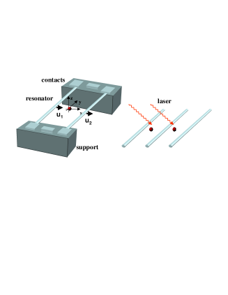
Figure 1: Setup. Left: ion trap with electrodes made of nanomechanical resonators suspended above ground and biased with ac voltage; right: arrays of nanomechanical resonators and laser manipulation of the trapped ions.

Model for ions coupled to nanomechanical electrodes: We consider a schematic setup as illustrated in Fig. 1, where an ion is trapped between two parallel suspended electrodes represented by nanowires or nanotubesnanowire_derHeer_Schoneburg_nanotube . When a gate voltage $V(t)=V_{0}\cos{\omega_{ac}t}$ with frequency $\omega_{ac}$ is applied to the electrodes via Ohmic contacts, the charge on the resonator oscillates with time and leads to oscillating forces on the ion as well as between the resonators. Averaging over the fast driving frequency results in an effectively harmonic trapping potential for the ion centered between the electrodes. According to Fig. 1 the resonators of radii $r_{0}$ are separated by a distance $2d_{0}$, much smaller than their length $2L_{0}$, and located a distance $h_{0}$ ($\leq L_{0}$) above the ground plane. As a consequence, there will be tight trapping of the motion of the ion along the $x$-axis (see Fig. 1) which couples to the high-$Q$ flexural (bending) modes of the electrodes, compared to looser confinement in orthogonal directions.

In Euler-Bernoulli theoryCleland_Roukes_noise the equation of motion for the (small) displacement $u_{i}(y)$ of the flexural modes of the $i$-th resonator ($i=1,2$) is given by $\partial^{2}u_{i}/\partial t^{2}+\left(EI_{2}/\rho\right)\partial^{4}u_{i}/\partial y^{4}=0$, where $E$ is Young’s modulus, $I_{2}$ the moment of inertia, and $\rho$ the mass density of the electrodesSchwab_Cleland_exp ; nanowire_derHeer_Schoneburg_nanotube . The $n$-th secular mode with the eigenfunction $u_{in}(y)$ has frequency $\omega_{in}=\sqrt{EI_{2}/\rho}q_{in}^{2}$ with wave vector $q_{in}$. We can expand the displacement of the electrode as $u_{i}\left(y\right)=\sum_{n}X_{in}u_{in}(y)$ where $X_{in}$ when quantized as $\hat{X}_{in}$ takes the role of a ”position” operator with a conjugate ”momentum” operator $\hat{P}_{in}$. The lowest flexural mode, also called the fundamental mode, has the secular function $u_{in=1}(y)=a_{0}\left[\cos{q_{i1}}\cosh{q_{i1}L}_{0}-\cosh{q_{i1}y}\cos{q_{i1}L}_{0}\right]$ where $a_{0}$ is the normalization coefficient and $q_{i1}\approx{(2\pi/L_{0})}0.376$. Note the flexural modes have quadratic dependence on the wave vector. Other acoustic phonons at long wave length are the longitudinal modes and the torsional modes which have much higher frequencies than flexural modes. For nanowires with the length of the order of $\mathrm{\mu m}$ the secular frequencies are in the range of tens to a few hundred MHz with quality factors $Q\geq 10^{4}$Schwab_Cleland_exp . For Carbon nanotube nanowire_derHeer_Schoneburg_nanotube ; Dresselhaus_books , the Young’s Modulus is $E=1\,\mathrm{TPa}$; with radius $r_{0}=2\,\mathrm{nm}$ and $2L_{0}=500\,\mathrm{nm}$ the fundamental mode has a frequency of $\omega_{b}=1\,\mathrm{\ GHz}.$

The vibration of two suspended resonators $i=1,2$ with mass $M_{i}$ and eigenmodes $\omega_{in}$ is described by the coupled parametric oscillator Hamiltonian

$$H_{v}\!=\!\sum_{i,n}\left(\frac{\hat{P}_{in}^{2}}{2M_{i}}\!+\!\frac{M_{i}\omega_{in}^{2}}{2}\hat{X}_{in}^{2}\right)\!+\!\sum_{m,n}\kappa_{mn}(t)\hat{X}_{1m}\hat{X}_{2n}$$ (1)

where the first term is the elastic energy and the second is a micromotion of the electrodes due to the electrostatic interaction between the oscillating charges on the resonators with $\kappa_{mn}(t)=\kappa_{mn}\cos^{2}\left(\omega_{ac}t\right)$. Explicit expression for the coefficients $\kappa_{mn}$ can be derived from an expansion of the electrostatic energy for given applied voltages $V_{i}(\equiv V(t))$, $E_{m}=-\frac{1}{2}\sum_{i,j}C_{ij}(\{\hat{X}_{in}\})V_{i}V_{j}$, with $C_{ij}$ capacitances of the resonators as functions of the displacements $\hat{X}_{in}$. For an array of electrodes, as in Fig. 1, these coupling terms may (partially) compensate each other due to symmetry considerations.

To derive the total Hamiltonian of the ion coupled to the electrodes we must consider the Coulomb interaction between the ion and the charge distribution on the resonators. The charge distribution on the $i$-th electrodes includes an (essentially uniform) charge density $\rho_{iv}\left(t\right)=\rho_{iv}\cos\omega_{ac}t$ induced by the time dependent external voltage, and an induced charge distribution $\rho_{iq}$ due to the presence of the ion (“image”charge). As mentioned above, we only consider the high frequency motion of the ion along the $x$-axis which is decoupled from the motion along $y$ and $z$. The interaction energy between the charge of the ion $q_{0}$ and the total charge density on the electrodes has the form $\sum_{i}\int ds_{i}\left(\rho_{iv}\left(t\right)+\rho_{iq}\right)q_{0}/4\pi\epsilon_{0}\left|R_{x}\hat{e}_{x}+y\hat{e}_{y}\right|$ with $R_{x}=\hat{x}+(-1)^{i+1}d_{0}-u_{i}\left(y\right)$, where we integrate along the resonator and the denominator involves the distance between the ion at position $\hat{x}\hat{e}_{x}$ (compare Fig. 1) and the electrode with displacement $u_{i}\left(y\right)\hat{e}_{x}$. For $\max\left(\left|u_{i}\left(y\right)\right|\right)\ll 2L_{0}$ the assumption of a constant charge distribution remains a good approximation. The interaction of the ion with the “image charge” is well approximated by $-q_{0}^{2}/4\pi\epsilon_{0}\left|R_{x}\right|\ln{(}\left|{R_{x}}\right|{/r_{0})}$image_charge_2002 and generates a small correction to the trapping and the coupling energy. An additional effect here is the modification of $\rho_{v}$ due to the small voltage of the image charge to the ground, which can be neglected for $h_{0}\gg d_{0}$.

Second order expansion in $\hat{x}$ and $\hat{X}_{ij}$ gives a harmonic coupling between the ion and the electrodes. The total Hamiltonian $H_{\mathrm{tot}}=H_{v}+H_{\mathtt{ion}}$ with $H_{\mathrm{ion}}$ the Hamiltonian for the ion of mass $m$ coupled to the electrodes

$$H_{\mathrm{ion}}=\frac{\hat{p}^{2}}{2m}+\frac{q_{0}(\widetilde{V}_{0}(t)+\widetilde{V}_{q})}{2d_{0}^{2}}\hat{x}^{2}+\sum_{in}g_{in}(t)\hat{X}_{in}\hat{x}$$ (2)

which includes the trapped ion Hamiltonian Hamiltonian with $\widetilde{V}_{0}(t)=2V_{ac}\cos{\omega_{ac}t}/\ln{(2h}_{0}\sqrt{h_{0}^{2}+d_{0}^{2}}{/r}_{0}d_{0}{)}$ modified by a (small) image charge contribution, $\widetilde{V}_{q}=-\alpha_{g}q_{0}/2\pi\epsilon_{0}d_{0}\ln{(d_{0}/r_{0})}$ (with $\alpha_{g}\approx 1$). The last term is the ion-electrode coupling with $g_{in}(t)=g_{in}\cos{\omega_{ac}t}$ and

$$g_{in}=\int_{i}dy\frac{q_{0}\rho_{iv}(t)(y^{2}-2d_{0}^{2})u_{in}(y)}{4\pi\epsilon_{0}(d_{0}^{2}+y^{2})^{5/2}}+\frac{q_{0}\widetilde{V}_{q}u_{in}\left(0\right)}{2d_{0}^{2}\ln{(d_{0}/r_{0})}}$$

where again the image charge gives a small modification. Note a displacement force $\sum g_{in}^{\left(1\right)}\cos\left(\omega_{ac}t\right)\hat{X}_{in}$ and an electrode-electrode interaction $\sum h_{i,mn}^{\left(2\right)}\cos\left(\omega_{ac}t\right)\hat{X}_{im}\hat{X}_{in}$ induced by the static ion, which can be derived by expanding the Coulomb interaction, are not written in Eq. (2).

We are interested in a situation where the trap frequency is near resonant with the lowest flexural mode $n=1$, while the driving field with frequency $\omega_{ac}$ is far off resonant with any of the other elastic eigenmodes. This, together with the fact that $g_{in}$ is a rapidly decreasing function of $n$, justifies the single mode approximation for the electrodes: $H_{\mathrm{ion}}=\hat{p}^{2}/2m+q_{0}\widetilde{V}_{0}\left(t\right)\left(\hat{x}-u_{1}(0)\hat{X}_{p}\right)^{2}/2d_{0}^{2}$, where $\hat{X}_{p}=(\alpha_{1}\hat{X}_{11}+\alpha_{2}\hat{X}_{21})/2$ and for symmetric electrodes and $d_{0}/L_{0}\leq 1$, $\alpha_{1}=\alpha_{2}\approx 1$. This Hamiltonian has the simple interpretation of a parametric oscillator where the trap center located at the center-of-mass (COM) displacement $\hat{X}_{p}$, providing a bilinear coupling of the ion to the electrodes.

As a final step, we adiabatically eliminate the (micro-)motion at the parametric drive frequency $\omega_{ac}$. We illustrate this for the case of two symmetric electrodes with identical eigenmode frequencies and masses, so that the ion only couples to the COM mode $\hat{X}_{p}$. We obtain for the effective Hamiltonian with coupling in the rotating wave approximation

$$H_{\mathrm{eff}}=\hbar\omega_{\nu}\hat{a}^{\dagger}\hat{a}+\hbar\omega_{b}\hat{b}^{\dagger}\hat{b}+(i\lambda\hat{b}^{\dagger}\hat{a}+\mathrm{h.c.})$$ (3)

where $\hat{b}$ ($\hat{b}^{{\dagger}}$) are the lowering (raising) operators of the COM flexural mode with mass $M_{p}=2M_{i}$; and $\hat{a}$ ($\hat{a}^{{\dagger}}$) operators for the harmonically trapped ion with frequency $\omega_{\nu}=q_{0}\widetilde{V}_{0}/\sqrt{2}d_{0}^{2}m\omega_{ac}$ and mass $m$. Near resonance at $\omega_{\nu}\sim\omega_{b}\ll\omega_{ac}$, the coupling is proportional to the trapping frequency while decreased by the mass ratio $m/M_{p}$: $\lambda=\hbar\omega_{\nu}u_{1}(0)\sqrt{m/M_{p}}$. This shows the nanomechanical resonator with lighter mass, e.g. a single wall carbon nanotube, will have stronger coupling with the trapped ion. Typical parameters are $V_{0}=5\,\mathrm{V}$, $\omega_{ac}/2\pi=3\,\mathrm{GHz}$, $d_{0}=100\,\mathrm{nm}$, $h_{0}=10d_{0}$, $r_{0}=2\,\mathrm{nm}$, $m/M_{p}\approx 10^{-4}$, and we have $\omega_{\nu}/2\pi=1\,\mathrm{GHz}$. The time dependent coupling $\kappa_{mn}\cos^{2}\omega_{ac}t$ in Eq. (1) satisfies $\left|\kappa_{mn}\right|\leq(Q_{c}/q_{0})\left(\omega_{ac}/\omega_{b}\right)m\omega_{b}^{2}\ll M_{p}\omega_{b}^{2}$ at $\omega_{\nu}\sim\omega_{b}$, where $Q_{c}=2L_{0}\rho_{v}$ is the charge on the electrodes from the voltage source. For the above numbers, $Q_{c}\approx 50$ and hence the $\kappa_{mn}$ term, so are the $\sum g_{in}^{(1)}$ and $h_{i,mn}^{(2)}$ terms, can be neglected due to the small mass ratio. In general, cantilever couplings are readily accounted for by transforming to a set of eigenmodes.

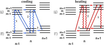
Figure 2: Energy structure of the combined system of the ion and the electrodes. Left: cooling circles; right:heating circles.

The coupled oscillator Hamiltonian (3) allows the transfer of the motional states of the electrodes and the ion. Motional states of the ions can be manipulated by coupling internal electronic states to a laser: $H_{I}=-\frac{1}{2}\delta\sigma_{z}+\Omega e^{i\eta(a+a^{{\dagger}})}\sigma^{+}+\mathrm{h.c.,}$ which can be added to Eq. (3). Here $\sigma$’s are the Pauli operators of the a two-state system, $\delta$ the laser detuning, $\Omega$ the Rabi frequency, and $\eta=k\sqrt{\hbar/2m\omega_{\nu}}$ the Lamb-Dick parameter describing the laser recoil on the ion motion. Based on these couplings, a complete toolbox is available on the ion for (i) quantum state engineering, and (ii) preparation of pure states (ground state cooling), and (iii) state measurements using the quantum jump technique. Preparing and analyzing motional states of the resonators are available via the transfer Hamiltonian when the coupling time $1/\lambda$ is faster than the decoherence time.

Decoherence: Decoherence of the nanomechanical resonator is induced by mechanicalCleland_Roukes_noise and electrical noiseBlanter_Buttiker_PR . The mechanical noise is characterized by the quality factor $Q$ due to the coupling with environments, such as the noise in the support of the electrodes and the surface of the electrodes. Electrical noiseBlanter_Buttiker_PR represents the voltage fluctuations on the electrodes, including the noise of the resistances in the circuit, shot noise and low frequency noise ($1/f$ noise). The shot noise is negligible for a ballistic electrode, i.e. single wall Carbon nanotubeBlanter_Buttiker_PR . The low frequency noise is due to charge fluctuations in the environment and the imperfection or dirt on the electrodes, and is negligible at GHz frequency.

Let $\delta\widetilde{v}_{i}\left(t\right)$ be the noise on the electrodes defined the same way as $\widetilde{V}_{0}$ with $i=1,2$. The voltage noise introduces: the parametric noise $q_{0}\delta\widetilde{v}_{p}\left(t\right)\left(\hat{x}-u_{1}\hat{X}_{p}\right)^{2}/2d_{0}^{2}$ with the spectrum $\delta\widetilde{v}_{p}^{2}\left(\omega\right)\approx\sum\delta\widetilde{v}_{i}^{2}\left(\omega\right)/4$, and the linear noise $q_{0}\delta\widetilde{v}_{m}\left(t\right)\left(\hat{x}-u_{1}\hat{X}_{p}\right)/2d_{0}$ with $\delta\widetilde{v}_{m}^{2}=\beta_{g}^{2}\sum\delta\widetilde{v}_{i}^{2}\left(\omega\right)/4$ and $\beta_{g}\approx 2\ln\left(2h_{0}/r_{0}\right)/\ln\left(2d_{0}/r_{0}\right)$, when $\delta\widetilde{v}_{1,2}\left(t\right)$ are not correlated. Due to $m/M_{p}\ll 1$, the $\hat{X}_{p}^{2}$, $\hat{x}\hat{X}_{p}$ and $\hat{X}_{p}$ terms are a factor of $m/M_{p}$ or $\left(m/M_{p}\right)^{2}$ smaller than the $\hat{x}^{2}$ and $\hat{x}$ terms, so we only consider the $\hat{x}^{2}$ and $\hat{x}$ terms. The parametric noise has a spectral density $\gamma_{1}(\omega)=\left(\delta x_{0}/d_{0}\right)^{4}q_{0}^{2}\delta\widetilde{v}_{p}^{2}\left(\omega\right)/4$. Due to the small ratio $\delta x_{0}/d_{0}$, $\gamma_{1}=0.5\mathrm{Hz}$ for the contact resistance at zero temperature and can be neglected. Here we have $R_{c}=h/2N_{\perp}e^{2}$ with $N_{\perp}$ the number of conducting channels and $N_{\perp}=4$ for Carbon nanotube, and $\delta\widetilde{v}_{p}^{2}\left(\omega\right)=R_{c}\omega/2$ at zero temperature. The linear term has a spectral density $\gamma_{m}(\omega)=\left(\delta x_{0}/d_{0}\right)^{2}q_{0}^{2}\delta\widetilde{v}_{m}^{2}\left(\omega\right)/4$, with $\delta\widetilde{v}_{m}^{2}\left(\omega\right)=R_{c}\omega/2$ for uncorrelated noise and $\gamma_{m}(\omega_{\nu})=0.5\mathrm{MHz}$. Note that due to the $\left(\delta x_{0}/d_{0}\right)^{2}$ factor, this term is stronger than the parametric noise. The linear noise can be avoided when the two electrodes are made of one piece of metallic wire connecting to only one contact. Now $\delta\widetilde{v}_{1}=\delta\widetilde{v}_{2}$, and $\gamma_{m}\sim 0$ as well as $\delta\widetilde{v}_{m}^{2}\sim 0$. Thus the condition of a decoherence time longer than the coupling time of the ion to the resonator can be met.

Resonator Cooling: The energy structure of the system is shown in Fig.2, where the state $\left|s,n,m\right\rangle$ corresponds to the internal state at $s$, the motion of the ion at the number state $n$, and the vibrational mode at the number state $m$. The states $\left|s,n,m\right\rangle$, $\left|s,n-1,m+1\right\rangle$ and $\left|s,n+1,m-1\right\rangle$ are connected by the coupling $\lambda$. Eliminating the internal degrees of freedom of the ions, the master equation in the interaction picture of the ion-resonator motion becomes

$$\begin{array}[]{r}\displaystyle\frac{\partial\rho}{\partial t}=-i\left[\lambda\hat{a}^{\dagger}\hat{b}+\mathrm{h.c.},\rho\right]+\mathcal{L}^{d}\left(\hat{a},\gamma_{\omega}^{\hat{a}},n_{f}\right)\rho\\ \displaystyle+\mathcal{L}^{d}\left(\hat{b},\frac{\omega_{B}}{Q},n_{B}\right)\rho+\mathcal{L}^{d}\left(\hat{a},\gamma_{m},n_{B}\right)\rho\end{array}$$ (4)

where we use the notation in Cirac_Blatt_Zoller_Phillips

$$\begin{array}[]{r}\displaystyle\mathcal{L}^{d}\left(A,\gamma_{\omega}^{A},n_{\omega}\right)\rho=\frac{1}{2}\gamma_{\omega}^{A}n_{\omega}\left(2A^{{\dagger}}\rho A-AA^{{\dagger}}\rho-\rho AA^{{\dagger}}\right)\\[5.69054pt] \displaystyle+\frac{1}{2}\gamma_{\omega}^{A}\left(n_{\omega}+1\right)\left(2A\rho A^{{\dagger}}-A^{{\dagger}}A\rho-\rho A^{{\dagger}}A\right)\end{array}$$

for the Liouvillian operators with the system operator $A$, noise spectrum $\gamma_{\omega}^{A},$ and a phonon number $n_{\omega}$. In Eq. (4) laser cooling of the ion contributes the $\mathcal{L}^{d}\left(\hat{a},\gamma_{\omega}^{\hat{a}},n_{f}\right)$ term, where $n_{f}$ is the final phonon number of the ion in the absence any additional heating mechanisms (i.e. $n_{f}\approx 0$) and cooling rate $\gamma_{\omega}^{\hat{a}}=\eta^{2}\Omega_{r}^{2}/\Gamma_{e}$ when $\Gamma_{e}>\eta\Omega_{r}$ is the rate of laser cooling. The linear voltage noise contributes the $\mathcal{L}^{d}\left(\hat{a},\gamma_{m},n_{B}\right)\$term. The resonator damping and heating contributes $\mathcal{L}^{d}\left(\hat{b},\gamma_{\omega}^{\hat{b}},n_{B}\right)$ where $\gamma_{\omega}^{\hat{b}}=\omega_{b}/Q$ and $n_{B}=k_{B}T/\hbar\omega_{b}$ is the thermal phonon number of the supports at frequency $\omega_{b}$.

For $n_{f}=0$, the final state phonon number of the electrodes is

$$\langle\hat{b}^{{\dagger}}\hat{b}\rangle_{f}=\frac{\displaystyle\left(\,\Gamma_{\nu}\,\gamma_{\mathrm{eff}}^{\hat{a}}\left(\gamma_{\mathrm{eff}}^{\hat{a}}+\Gamma_{\nu}\right)+4\Gamma_{\nu}\lambda^{2}\right)n_{B}+4\,\,\gamma_{\mathrm{eff}}^{\hat{a}}\,{\lambda}^{2}n_{f}^{\mathrm{eff}}}{\displaystyle{\left(\Gamma_{\nu}+\gamma_{\mathrm{eff}}^{\hat{a}}\right)}\left(\gamma_{\mathrm{eff}}^{\hat{a}}\Gamma_{\nu}+4\lambda^{2}\right)}$$

with $\Gamma_{v}=\omega_{b}/Q$. The effective cooling rate is $\gamma_{\mathrm{eff}}^{\hat{a}}=$ $\gamma_{\omega}^{\hat{a}}+\gamma_{m}$ including the voltage noise with the final phonon number of the ion $n_{f}^{\mathrm{eff}}=n_{B}\gamma_{m}/\gamma_{\mathrm{eff}}^{\hat{a}}$. When $\gamma_{m}\sim\gamma_{\mathrm{eff}}^{\hat{a}}$ the ion can not be cooled and hence the electrodes. As a necessary requirement we need $\gamma_{m}\sim 0$, i.e. the two electrodes in one piece (see above). In this case, when $\gamma_{\omega}^{\hat{a}}=2\lambda$ the stationary phonon number is minimized: $\langle\hat{b}^{{\dagger}}\hat{b}\rangle_{\min}=\left(k_{B}T/Q\right)(4\lambda+\Gamma_{\nu})/\left(2\lambda+\Gamma_{\nu}\right)^{2}$. With our parameters $\Gamma_{e}=5\,\mathrm{MHz}$, $\Omega_{r}=300\,\mathrm{MHz}$, and $\gamma_{\omega}^{\hat{a}}=2\mathrm{MHz}$, we have $\langle\hat{b}^{{\dagger}}\hat{b}\rangle_{f}\approx 0.5$ with $Q=10^{5}$ and $\mathrm{T}=4\mathrm{K}$.

For the high trapping frequencies, the Lamb-Dicke parameter is small with $\eta\sim 0.01$ and as a result $\gamma_{\omega}^{\hat{a}}<\lambda$. The ion cooling rate becomes the bottleneck for the cooling process. The problem can be avoided by trapping the ion at low frequency $\omega_{\nu}\ll\omega_{b}\sim\omega_{ac}$ (and thus large $\eta$). The ac driving field provides a parametric up-conversion of the ion to the resonator phonons, i.e. $\lambda\longrightarrow\hbar\omega_{\nu}u_{1}\sqrt{m\omega_{ac}^{2}/M_{p}\omega_{b}\omega_{\nu}}e^{-i\omega_{ac}t}$ in Eq. (3).

Entanglement generation: Quantum state engineering of ion can be used to generate entangled states of the resonators via the coupling Eq. (3). For example, let us discuss the generation of $\left|\psi_{1},\chi_{2}\right\rangle+\left|\chi_{1},\psi_{2}\right\rangle$ for two resonators where $\left|\psi_{i}\right\rangle$ and $\left|\chi_{i}\right\rangle$ are arbitrary states of the electrode $i=1,2$. We choose the electrodes to have different fundamental frequency $\omega_{b1}\neq\omega_{b2}\,$ and coupling with the ion $\lambda_{i}$. The initial state $\left(\left|\uparrow,\psi_{x}\right\rangle+\left|\downarrow,\chi_{x}\right\rangle\right)\left|0_{1},0_{2}\right\rangle$ with $x$ for the motion of the ion is prepared using standard protocols of the ion trap qubitsEberly_Law_Cirac_Zoller , where the motional and the internal state of the ion are entangled. In a first step we tune the ion to the first resonator resonance $\omega_{\nu}=\omega_{b1}$ for a duration of $\pi/2\lambda_{1}$, which results in the swap $\left|n_{x},m_{1}\right\rangle\rightarrow\left|m_{x},n_{1}\right\rangle$, and the state is now $\left(\left|\uparrow,0_{x},\psi_{1}\right\rangle+\left|\downarrow,0_{x},\chi_{1}\right\rangle\right)\left|0_{2}\right\rangle$. Now we prepare the state $\left(\left|\uparrow,\chi_{x},\psi_{1}\right\rangle+\left|\downarrow,\psi_{x},\chi_{1}\right\rangle\right)\left|0_{2}\right\rangle$ via a third internal state in the ionEberly_Law_Cirac_Zoller . Then, we tune the trapping frequency to $\omega_{\nu}=\omega_{b2}$ for a duration of $\pi/2\lambda_{2}$, which results in $\left|n_{x},m_{2}\right\rangle\rightarrow\left|m_{x},n_{2}\right\rangle$, and the state is $\left(\left|\uparrow,0_{x},\psi_{1},\chi_{2}\right\rangle+\left|\downarrow,0_{x},\chi_{1},\psi_{2}\right\rangle\right)$. Now we rotate the internal state by a $\pi/2$ pulse: $\left|\uparrow\right\rangle\rightarrow\left|\uparrow+\downarrow\right\rangle$ and $\left|\downarrow\right\rangle\rightarrow\left|\uparrow-\downarrow\right\rangle$; then detect the internal state. The detection generates states $\left|\psi_{1},\chi_{2}\right\rangle\pm\left|\chi_{1},\psi_{2}\right\rangle$ depending on the detected internal states; and entanglement is transferred from the ion to the resonators. This method can be applied to generate for example $\left|0_{1},n_{2}\right\rangle+\left|n_{1},0_{2}\right\rangle$ as entangled state of the two electrode modes. The entanglement can be achieved on a time scale of $\pi/\lambda_{1,2}\approx 50\mathrm{n}\sec$. Given a decoherence time of $1\mathrm{MHz}$, a fidelity exceed $0.9$ can be achieved.

Quantum Computing: Mesoscopic traps promise trap frequencies significantly higher than those of present ion traps and an associated speed up of two-qubit gates in ion trap quantum computing (Fig. 1). The standard 2-qubit protocols based on, for example, entanglement via a phonon data bus or a push gate are readily adapted to the present case. In the second case, gate times of the order of nanoseconds seem possible for the numbers above. A second possibility is entanglement via exchange of phonons of one of the collective ion-electrode modes of the system. Additional noise is, however introduced by the mechanical motion. The decoherence of the ion motion when in resonance with one mode $\omega_{\nu}=\omega_{i1}$ is $\tau_{res}^{-1}=k_{B}T/Q$ which is $1\mathrm{MHz}$ with $Q=10^{5}$ and assuming the same quality factor for two electrodes. When off resonance $\left|\omega_{i1}-\omega_{\nu}\right|>k_{B}T/Q$, the decoherence rate is

$$\Gamma_{m}=\frac{k_{B}T}{Q}\frac{m}{M_{p}}\sum_{i,n}\frac{u_{i_{b}}^{2}(0)\omega_{\nu}^{3}\omega_{i_{n}}}{(\omega_{\nu}^{2}-\omega_{in}^{2})^{2}+4\omega_{in}^{2}\left(\frac{k_{B}T}{Q\hbar}\right)^{2}}$$ (5)

so that the decoherence rate is $\Gamma_{m}\approx(8u_{1}^{2}m/9M_{p})\left(k_{B}T/Q\right)\sim 2\pi\cdot 100\,\mathrm{Hz}$ with $\omega_{i1}=500\,\mathrm{MHz}$ and $\omega_{\nu}=1\,\mathrm{GHz}$. The small mass ratio $m/M_{p}$ and the off resonance protect the ion from decoherence. The decoherence due to the electrical noise is, dominated by $4\gamma_{1}\left(0\right)=2\pi\cdot 0.1\mathrm{Hz}$ assuming a low frequency noise $\left(q_{0}^{2}\delta\widetilde{v}_{1}^{2}\left(0\right)\right)^{-1}=1\mathrm{n}\sec$. Hence, the decoherence time is much longer in the nano trap. This shows that the smallest charge box – single ion – coupling with the nanomechanical resonators not only presents an effective knob for quantum features of the flexural modes, but also increases the speed of ion trap quantum computing by several orders of the magnitudes.

Acknowledgments: We thank M.S. Dresselhaus, B.I. Halperin, D. Leibfried, L.S. Levitov, M.D. Lukin, A.S. Sørensen, and W. Zwerger for helpful discussions. This work is supported by the Austrian Science Foundation, European Networks and the Institute for Quantum Information.

References

• (1) J. I. Cirac and P. Zoller, Phys. Today March vol.57, 38 (2004).
• (2) M. D. Barrett et al., Nature 429, 737 (2004); M. Riebe et al., Nature 429, 734 (2004)
• (3) D. Kielpinski et al., Nature 417, 709 (2002); J. I. Cirac and P. Zoller, Nature 404, 579 (2000).
• (4) D.J. Wineland et al., J. Res. Natl. Inst. Stand. Technol. 103, 259 (1998), see sect. 6.4, pp319; L. Tian and et al., Phys. Rev. Lett. 92, (2004) 247902; A. S. SΓΈrensen et al., Phys. Rev. Lett. 92, 063601 (2004).
• (5) M.D. LaHaye et al., Science 304, 74 (2004); R.G. Β Knobel and A.N. Cleland, Nature 424, 291 (2003).
• (6) A. Husain et al., Appl. Phys. Lett. 83, 1240 (2003); P.Β Poncharal et al., Science 283, 1513 (1999); B.Β Babic et al., Nano Lett. 3, 1577 (2003).
• (7) A.N. Cleland and M.L. Roukes, J. Appl. Phys. 92, 2758 (2002).
• (8) R. Saito et al., Physical Properties of Carbon Nanotubes, Imperial College Press, London (1998); MRS Bulletin 29, Advances in Carbon Nanotubes, April 2004.
• (9) B.E. Granger et al., Phys. Rev. Lett. 89, 135506 (2002).
• (10) Ya. M. Blanter and M. BΓΌttiker, Phys. Rep. 336, 1 (2000).
• (11) J. I. Cirac et al., Phys. Rev. A 46, 2668 (1992).
• (12) C. K. Law and J. H. Eberly, Phy. Rev. Lett. 76, 1055 (1996); J. I. Cirac and P. Zoller, Phys. Rev. Lett. 74, 4091 (1995).