The Extent of Multi-particle Quantum Non-locality

Abstract

It is well known that entangled quantum states can be nonlocal: the correlations between local measurements carried out on these states cannot always be reproduced by local hidden variable models. Svetlichny, followed by others, showed that multipartite quantum states are even more nonlocal than bipartite ones in the sense that nonlocal classical models with (super-luminal) communication between some of the parties cannot reproduce the quantum correlations. Here we study in detail the kinds of nonlocality present in quantum states. More precisely we enquire what kinds of classical communication patterns cannot reproduce quantum correlations. By studying the extremal points of the space of all multiparty probability distributions, in which all parties can make one of a pair of measurements each with two possible outcomes, we find a necessary condition for classical nonlocal models to reproduce the statistics of all quantum states. This condition extends and generalises work of Svetlichny and others in which it was shown that a particular class of classical nonlocal models, the “separable” models, cannot reproduce the statistics of all multiparticle quantum states. Our condition shows that the nonlocality present in some entangled multiparticle quantum states is much stronger than previously thought. We also study the sufficiency of our condition.

I Introduction

A natural way of characterizing the correlations present in entangled quantum states is to attempt to replicate their measurement statistics using classical models. Bell B showed that classical models respecting relativistic causality - often called local hidden variable (lhv) models - cannot always reproduce quantum statistics. If the classical model allows unlimited (superluminal) communication between the parties then the quantum correlations can be reproduced trivially. More refined studies attempt to understand exactly what superluminal classical communication will reproduce the quantum correlations. In the bipartite case, efforts have concentrated on the number of bits of communication required to reproduce the quantum correlations Brass ; Stein ; Mass ; Toner . In the three party setting Svetlichny Svet showed that, even allowing superluminal communication between arbitrary pairs of parties cannot reproduce the results of measurements performed on quantum states. Two papers independently generalised Svetlichny’s result to an arbitrary number of parties Seev ; Col .

In the present work we refine this analysis by showing that the class of classical correlations that cannot reproduce the quantum correlations is much larger than the separable class considered in Svet ; Seev ; Col . We show that, not only is the non-locality of multi-particle quantum correlations stronger than previously thought, but also there is a way of categorizing non-local correlations using graphs of communication.

Let us first recall Bell’s idea. Consider $m$ parties which each receive as input a measurement setting $x_{i}$ and produce an output $a_{i}$. The probability of a certain outcome for a given set of settings is:

$$P(\vec{a}|\vec{x})=P(a_{1},...,a_{m}|x_{1},...,x_{m}).$$ (1)

One way to generate such correlations is for the parties to share an entangled quantum state. Depending on his input, each party then carries out a measurement on the quantum state. The result of the measurement is his output. We denote the quantum mechanical correlations obtained in this way by $P_{qm}$.

The most general way of generating correlations using only classical resources, without any signalling taking place between the parties, is for the parties to share a prior random variable $\lambda$ (often called the hidden variable). Each party then chooses its outcome depending on its input and on $\lambda$. The set of correlations produced using such local hidden variable models has the form:

$$P_{lhv}(\vec{a}|\vec{x})=\tiny\int d\lambda P(a_{1}|x_{1},\lambda)P(a_{2}|x_{2},\lambda)..P(a_{m}|x_{m},\lambda)\rho(\lambda),$$ (2)

where $\rho(\lambda)$ is a probability distribution over the variables $\lambda$.

Note that neither the quantum nor the lhv models allow signalling, since in neither of the models does any communication take place between the parties after they receive their input. Bell’s central result was to show that some quantum correlations cannot be reproduced by lhv models. This is proved by introducing an inequality -called a “Bell inequality”- which must be satisfied by the lhv models but which is violated by the quantum correlations. See for instance Wolf ; Zuk for all “correlation inequalities” in the multipartite case.

Svetlichny Svet generalised and refined Bell’s result in the three party setting by showing that some three-party quantum correlations cannot be reproduced classically, even if communication, about settings and results, is allowed between a pair of parties. The two parties in communication need not be fixed in advance, but can be chosen with probabilities $p_{i}$. The correlations considered by Svetlichny are thus of the form:

$$P_{Svet}(\vec{a}|\vec{x})=$$

$$\int d\lambda\big{[}p_{1}\rho_{1}(\lambda)P_{1}(a_{1}|x_{1},\lambda)P_{1}(a_{2},a_{3}|x_{2},x_{3},\lambda)$$

$$+p_{2}\rho_{2}(\lambda)P_{2}(a_{2}|x_{2},\lambda)P_{2}(a_{1},a_{3}|x_{1},x_{3},\lambda)$$

$$+p_{3}\rho_{3}(\lambda)P_{3}(a_{3}|x_{3},\lambda)P_{3}(a_{1},a_{2}|x_{1},x_{2},\lambda)\big{]}\ .$$ (3)

Here $P(a_{2},a_{3}|x_{2},x_{3},\lambda)$, and the two terms like it, can be $any$ probability distribution (it need not separate into $P_{1}(a_{2}|x_{2},\lambda)P_{1}(a_{3}|x_{3},\lambda)$ note that ). The main result of Svetlichny Svet is to show that there are quantum states (e.g. the Greenberger-Horne-Zeilinger state $(1/\sqrt{2})(\left|000\right\rangle+\left|111\right\rangle)$; see Pop for a proof that this is the optimal state for this purpose) with $P_{qm}(\vec{a}|\vec{x})$ such that no distribution $P_{Svet}(\vec{a}|\vec{x})$ can be found such that $P_{qm}=P_{Svet}$ for all $\vec{x}$. This is proved by introducing an inequality - called a “Sveltichny inequality”- which must be satisfied by correlations of the form eq. (3) but can be violated by quantum correlations. Thus even allowing some non-local, ie. superluminal, classical communication between pairs of parties, one cannot reproduce all three party quantum correlations.

Refs. Seev ; Col extended the hybrid local/non-local model of Svetlichny to the $m$-party setting. They allowed arbitrary communication within disjoint subsets of the parties, but each subset was independent of the settings and results of other subsets. In Collins et al. these correlations were termed “separable”. It was shown that the GHZ state has measurement statistics which cannot be reproduced by these models. Sets of correlations which are not separable will be called “inseparable”.

In the present paper we will show that there are many inseparable correlations which cannot reproduce quantum correlations. More precisely we will define a class of “Partially Paired” correlations $P_{PP}(\vec{a}|\vec{x})$, which include the separable correlations and some inseparable correlations, and categorize them in terms of networks of communication. Using a generalised Svetlichny inequality, taken from Col , we show that this class cannot reproduce all quantum correlations. We will also show that the complement of this class, the “Totally Paired” correlations, $P_{TP}(\vec{a}|\vec{x})$ maximally violate these inequalities. These generalised Svetlichny inequalities therefore cannot discriminate between models in $TP$ and quantum correlations. The class $TP$, unlike $PP$, is thus a good candidate for a classical description of all quantum correlations.

Our results are based on two advances; first we have formulated an intuitive graphical means of classifying multi-particle correlations allowing us to define $PP$ and $TP$; second we developed a deeper understanding of the multi-particle Svetlichny Inequality and the set of all similar inequalities. Both of these advances promise results beyond the scope of this paper.

In the following we first introduce some of the basic conceptual tools we shall use in our work (II,III), we then sketch our results in the four-party case (IV,V) before providing full proofs for $m$-parties (VI,VII).

II Geometry of the space of correlations

Consider $m$ parties, each of which receives an input $x_{i}$ and produces an output $a_{i}$. The outputs can be correlated to the inputs in an arbitrary way. Hence the most general way of describing such a situation, independently of any underlying physical model, is by a set of probability distributions $P(\vec{a}|\vec{x})$. The starting point of our investigation is to describe, in detail, the geometry of the set of such probability distributions.

The set of probability distributions is characterised by the normalisation conditions:

$$\sum_{\vec{a}}P(\vec{a}|\vec{x})=1,$$ (4)

and the positivity conditions:

$$P(\vec{a}|\vec{x})\geq 0\ .$$ (5)

Therefore the set of possible probability distributions is a convex polytope. This polytope belongs to the subspace defined by eq. (4). Its facets are given by equality in (5).

It is useful to find the extreme points of this polytope. These are the probability distributions which saturate a maximum of the positivity conditions, eq. (5), while satisfying the normalisation conditions, eq. (4). It is easy to see that the extreme points are the probability distributions such that, for each $\vec{x}$, there is a unique $\vec{a}=\vec{a}(\vec{x})$ with $P(\vec{a}|\vec{x})=1$ (and therefore if $\vec{a}\neq\vec{a}(\vec{x})$ then $P(\vec{a}|\vec{x})=0$). Thus there is a one to one correspondence between the set of extreme points and the functions $\vec{a}(\vec{x})$ from the inputs to the outputs. Any particular $\vec{a}(\vec{x})$ defines an extreme point. We call the extreme points deterministic models since there is no randomness in this case: the output is completely fixed by the input. We will soon associate a graph with families of extreme points.

Subspaces of the space of all distributions satisfying normalisation and positivity can be defined by taking all convex combinations of a subset of the extreme points. This is a natural construction because, if a physical model can produce certain extreme points, then it can produce any convex combination of these extreme points simply by randomly choosing which extreme point to realize.

A first interesting example is the subspace defined by lhv models. The corresponding extreme points are of the form $a_{i}(\vec{x})=a_{i}({x_{i}}$): the measurement results of party $i$ depend only on the settings of that party.

A second example subspace is provided by the separable correlations considered by Svetlichny and in Seev ; Col . The corresponding extreme points can be characterised as follows. For each extreme point there is a partition of the set of all parties into two subsets, say $\{1,...,k\}$ and $\{k+1,...,m\}$, such that $a_{i}(\vec{x})=a_{i}(x_{1},...,x_{k})$ if $i\in\{1,...,k\}$ and $a_{i}(\vec{x})=a_{i}(x_{k+1},...,x_{m})$ if $i\in\{k+1,...,m\}$. In the former situation, party $i$ has results, $a_{i}$, independent of the settings of the set $\{k+1,...,m\}$ and dependent on the settings $(x_{1},...,x_{k})$.

Note that the formulation given by Svetlichny, see eq. (3), and by Seev ; Col may seem more general than this since in their formulation the outputs of any party in set $\{1,...,k\}$ can depend on the inputs and outputs of all parties $1,...,k$ whereas above we have only allowed the outputs of any party in set $\{1,...,k\}$ to depend on the inputs of all parties $1,...,k$.

Let us now show that this is not the case, and that the two formulations are equivalent. For definiteness we will focus on the three party case, eq. (3), but the argument immediately extends to an arbitrary number of parties. Consider the set of probabilities $P_{1}(a_{1}|x_{1}\lambda)$, $P_{1}(a_{2},a_{3}|x_{2},x_{3},\lambda)$ etc., appearing in equation (3). The key point to note is that we can take these probabilities to be deterministic strategies. Indeed we have just argued that any probability can be written as a convex combination of extremal probabilities: $P_{1}(a_{2},a_{3}|x_{2},x_{3},\lambda)=\sum_{\mu}p_{\lambda}(\mu)P_{\mu}^{ext}(a_{2},a_{3}|x_{2},x_{3})$, where $p_{\lambda}(\mu)$ is a probability distribution over $\mu$ and where $P^{ext}_{\mu}(a_{2},a_{3}|x_{2},x_{3})$ equals zero except if $a_{2}=a_{2}(x_{2},x_{3})$ and $a_{3}=a_{3}(x_{2},x_{3})$. One can now suppose that the variables, $\mu$, which specify the weighting of each extremal probability, are included in the lhv variable $\lambda$, i.e. the lhv tells the parties in each set what deterministic strategy they must use. We have now proved our claim since, in the case of extremal correlations, each output depends only on the inputs of the parties, not on their outputs. Thus in the case of separable correlations, letting the outputs of the parties in each set depend only on the inputs of the parties in their set is completely general: there is no need to also let them depend on the outputs of the parties in the set.

We now introduce new subspaces of the probability distributions which form the basis for the present analysis.

III Classifying probability distributions using communication patterns

We will classify the extremal points by the settings that each variable $a_{i}$ depends on. This dependence can be represented using directed graphs. An arrow from party $i$ to $j$ means that $a_{j}$ depends on the setting $x_{i}$. If there is no arrow from $i$ to $j$, $a_{j}$ is independent of $x_{i}$ (changing the value of $x_{i}$ only, leaves $a_{j}$ unaltered). The graph is directed as one might have $a_{i}(x_{j})$ but $a_{j}$ independent of $x_{i}$ (an arrow $j\rightarrow i$ but no arrow $j\leftarrow i$). We call such a graph a communication pattern.

Any such communication pattern can be associated naturally to a model in which

i) Each party receives its input.

ii) If there is an arrow $i\rightarrow j$, $i$ sends its input to $j$.

iii) The parties which receive arrows produce their measurement results conditional on the list of inputs sent to them and their own input.

Steps ii),iii) should be thought of as a single-shot mail strategy: all of the settings are posted at the same time, along the appropriate arrow, and they are received at the same time. On receipt, the parties immediately generate their results: there is no communication about the results obtained. It is now clear why the arrows are directed: $i$ sending a letter to $j$ does not imply that $j$ mails $i$. Note that this single-shot mailing has to be superluminal if the measurements take place simultaneously and at spatially separated locations.

Note that any particular graph represents many extreme points. Indeed each extreme point corresponds to a unique function $\vec{a}=\vec{a}(\vec{x})$ whereas each graph only determines the variables the functions $\vec{a}$ depend on.

A formalisation of the above will prove useful. A given graph $G$ represents a set, $E_{G}$, of extreme points. Each point is identifiable with a different function $\vec{a}(\vec{x})$. These extreme points can be combined in convex combinations to make different distributions $P(\vec{a}|\vec{x})$ for each $\vec{x}$. The set of all such correlations produced by convex combinations of the extremal points $E_{G}$ will be called $C_{G}$: the set of correlations of type $G$. It is important to note that we define the set $E_{G}$ as including the extremal points represented by all subgraphs of $G$. For example, the graph $F$, in which all points send arrows to all others (Fig. $1v$), represents the set of all extreme points. Hence $C_{F}$ is the space of all correlations.

Different models, such as lhv models B or separable models Svet ; Seev ; Col can be associated with different classes of graphs. This is illustrated in the case of 4 parties in Fig. 1. The notation $a_{1}(x_{1},\wedge,\wedge,x_{4})$ is to be read as ‘party $1$’s outcome is independent of the settings of parties $2,3$ but dependent on the settings of $1,4$’, ie. $a_{1}$ is unaltered by changes in $x_{2},x_{3}$.

Figure 1: i) This graph represents the set of extreme points identifiable with lhv models, ie. $a_{i}(x_{i})$. Bell considered convex combinations of these points. ii a) and b) These graphs represent functions $\vec{a}(\vec{x})$ with the structure $a_{1}(x_{1},\wedge,x_{3},\wedge)$, $a_{3}(x_{1},\wedge,x_{3},\wedge)$, $a_{2}(\wedge,x_{2},\wedge,x_{4})$, $a_{4}(\wedge,x_{2},\wedge,x_{4})$ and $a_{1}(x_{1},x_{2},x_{3},\wedge)$, $a_{3}(x_{1},x_{2},x_{3},\wedge)$, $a_{2}(x_{1},x_{2},x_{3},\wedge)$, $a_{4}(\wedge,\wedge,\wedge,x_{4})$ respectively. Col considers correlations which are convex combinations of extremal points represented by separable graphs of this form and show that such models have $\langle S_{4}\rangle\leq 2$ (see Section IV)  iii) This graph represents functions $\vec{a}(\vec{x})$ which have $a_{1}(x_{1},x_{2},x_{3},\wedge)$, $a_{3}(x_{1},x_{2},x_{3},\wedge)$, $a_{2}(x_{1},x_{2},\wedge,x_{4})$, $a_{4}(x_{1},x_{2},\wedge,x_{4})$. Parties $3$ and $4$ are separated in the sense that no party receives arrows from both. We will show that convex combinations of these extreme points yield a value of $\langle S_{4}\rangle\leq 2$. We call graphs of type i)-iii) ‘Partially Paired’.  iv) Examples of graphs in which there is always a party which knows the settings of any pair - we call these ‘Totally Paired’. Certain convex combinations of the extremal points represented by these graphs can achieve the algebraic maximum $\langle S_{4}\rangle=4$, as described in the text. a) $a_{1}(x_{1},x_{2},x_{3},x_{4})$, $a_{3}(\wedge,\wedge,x_{3},\wedge)$, $a_{2}(\wedge,x_{2},\wedge,\wedge)$, $a_{4}(\wedge,\wedge,\wedge,x_{4})$ b) $a_{1}(x_{1},\wedge,x_{3},\wedge)$, $a_{3}(\wedge,x_{2},x_{3},x_{4})$, $a_{2}(x_{1},x_{2},\wedge,\wedge)$, $a_{4}(x_{1},x_{2},\wedge,x_{4})$  v) This graph represents the set of all extreme points and all possible 4-party graphs are its subgraphs.

IV Four Party Case: the Svetlichny inequality

Our study of multi-particle non-locality is based on combining the classification of correlations in terms of communication patterns with the Svetlichny inequality Svet and its generalisation described in Seev ; Col . We now illustrate this connexion in the case of 4 parties.

From now on we restrict ourselves to the case where each party’s input is a single bit $x_{i}\in\{0,1\}$ and each party’s output is a single bit $a_{i}\in\{0,1\}$. In order to make contact with earlier work we introduce an alternative notation.

First of all it is useful to suppose that the outputs have values $+1,-1$ instead of $0,+1$. In this case we denote the output of party $i$ by $A_{i}$ with the correspondence $A_{i}=(-1)^{a_{i}}$.

Secondly we denote by a superscript $x_{i}$ on $A_{i}$ (i.e. $A_{i}^{x_{i}}$) the value of the input of party $i$. This traditional notation is good in the case of lhv models, since each output $A_{i}$ is uniquely determined by its input. But it is somewhat unnatural for other models where $A_{i}$ can depend on the inputs of all parties and not only on $x_{i}$. However the product of four outputs such as $A_{1}^{1}A_{2}^{1}A_{3}^{0}A_{4}^{0}$ is well defined in this notation since all inputs are specified. The expression $A_{1}^{1}A_{2}^{1}A_{3}^{0}A_{4}^{0}$ denotes the product of the outputs of parties $1,2,3$ and $4$ given that the inputs are $(x_{1},x_{2},x_{3},x_{4})=(1,1,0,0)$.

We will be interested in the Svetlichny polynomials which are specific combinations of all products $A_{1}^{x_{1}}A_{2}^{x_{2}}A_{3}^{x_{3}}A_{4}^{x_{4}}$. In the case of four parties the Svetlichny polynomial is

$$S_{4} = \frac{1}{4}\Big{[}A_{1}^{0}A_{2}^{0}(-A_{3}^{0}A_{4}^{0}+A_{3}^{0}A_{4}^{1}+A_{3}^{1}A_{4}^{0}+A_{3}^{1}A_{4}^{1})$$ (6)

$$\;\;+A_{1}^{1}A_{2}^{0}(A_{3}^{0}A_{4}^{0}+A_{3}^{0}A_{4}^{1}+A_{3}^{1}A_{4}^{0}-A_{3}^{1}A_{4}^{1})$$

$$\;\;+A_{1}^{0}A_{2}^{1}(A_{3}^{0}A_{4}^{0}+A_{3}^{0}A_{4}^{1}+A_{3}^{1}A_{4}^{0}-A_{3}^{1}A_{4}^{1})$$

$$\;\;-A_{1}^{1}A_{2}^{1}(-A_{3}^{0}A_{4}^{0}+A_{3}^{0}A_{4}^{1}+A_{3}^{1}A_{4}^{0}+A_{3}^{1}A_{4}^{1})\Big{]}$$

$$= \sum_{\vec{x}}F_{4}(\vec{x})A_{1}^{x_{1}}A_{2}^{x_{2}}A_{3}^{x_{3}}A_{4}^{x_{4}}\ .$$

The expectation value of the Svetlichny polynomial is obtained by taking the average over all possible inputs and outputs weighted by the corresponding probabilities. Explicitly this can be written as

$$\langle S_{4}\rangle=\sum_{\vec{x}}F_{4}(\vec{x})(-1)^{a_{1}}(-1)^{a_{2}}(-1)^{a_{3}}(-1)^{a_{4}}P(\vec{a}|\vec{x})$$ (7)

The basis of our analysis will be to compare the maximum value of the Svetlichny polynomial attained by different models. Note that since $\langle S_{4}\rangle$ is a linear function of the probabilities $P(\vec{a}|\vec{x})$, its maximum value when the $P(\vec{a}|\vec{x})$ belong to a convex space will be attained on the extreme points of this space. This is the main justification for classifying correlations according to their extreme points: Bell type expressions obtain their maximum value on the extreme points.

It is easy to show that in the case of lhv models $\langle S_{4}\rangle\leq 2$. Collins et al. show that for separable models, $\langle S_{4}\rangle\leq 2$. And for certain quantum states the value of $\langle S_{4}\rangle=2^{\frac{3}{2}}$ Pop . We will show that much more general non-local models than the separable models considered in Seev ; Col also have $\langle S_{4}\rangle\leq 2$. Thus quantum mechanical states can exhibit even more general types of non-locality than previously anticipated.

V Four party case: Communication patterns and the Svetlichny inequality

Collins et al. showed that the set of correlations of type Fig. 1i),iia),iib) describe statistics of ‘separable’ physical models that cannot simulate all quantum states. We will now show that, despite being much more correlated than ii), no extreme point represent by graph iii) has a larger maximum value for $S_{4}$. Below is a sketch of a proof, details being saved for the $m$-party setting.

Consider a deterministic setting, $\vec{a}=\vec{a}(\vec{x})$, characterised by the graph iii) where $a_{1}=a_{1}(x_{1},x_{2},x_{3},\wedge)$, $a_{3}=a_{3}(x_{1},x_{2},x_{3},\wedge)$, $a_{2}=a_{2}(x_{1},x_{2},\wedge,x_{4})$, $a_{4}=a_{4}(x_{1},x_{2},\wedge,x_{4})$. Noting the form of the $a_{i}$, the following term from (6),

$$\frac{1}{4}A_{1}^{0}A_{2}^{0}(-A_{3}^{0}A_{4}^{0}+A_{3}^{0}A_{4}^{1}+A_{3}^{1}A_{4}^{0}+A_{3}^{1}A_{4}^{1}),$$ (8)

can be rewritten as:

$$\frac{1}{4} \Big{[}-(-1)^{a_{1}(0,0,0,\wedge)+a_{2}(0,0,\wedge,0)+a_{3}(0,0,0,\wedge)+a_{4}(0,0,\wedge,0)}$$

$$+ (-1)^{a_{1}(0,0,0,\wedge)+a_{2}(0,0,\wedge,1)+a_{3}(0,0,0,\wedge)+a_{4}(0,0,\wedge,1)}$$

$$+ (-1)^{a_{1}(0,0,1,\wedge)+a_{2}(0,0,\wedge,0)+a_{3}(0,0,1,\wedge)+a_{4}(0,0,\wedge,0)}$$

$$+ (-1)^{a_{1}(0,0,1,\wedge)+a_{2}(0,0,\wedge,1)+a_{3}(0,0,1,\wedge)+a_{4}(0,0,\wedge,1)}\Big{]}.$$ (9)

One can now find the maximum value of this expression. Defining $a_{1}(0,0,x_{3},\wedge)+a_{3}(0,0,x_{3},\wedge)\;\;\rm mod\rm\;\;2=\beta_{1}(x_{3})$ and $a_{2}(0,0,\wedge,x_{4})+a_{4}(0,0,\wedge,x_{4})\;\;\rm mod\rm\;\;2=\beta_{2}(x_{4})$ (this approach will be reused later) this expression simplifies to:

$$\frac{1}{4}\Big{[}-(-1)^{\beta_{1}(0)+\beta_{2}(0)}+(-1)^{\beta_{1}(0)+\beta_{2}(1)}$$

$$+(-1)^{\beta_{1}(1)+\beta_{2}(0)}+(-1)^{\beta_{1}(1)+\beta_{2}(1)}\Big{]}.$$ (10)

One now notes that, whatever the value of functions $\beta_{i}$, this expression is $\leq\frac{1}{2}$. Similarly each of the three other terms in $S_{4}$:

$$\frac{1}{4}A_{1}^{1}A_{2}^{0}(A_{3}^{0}A_{4}^{0}+A_{3}^{0}A_{4}^{1}+A_{3}^{1}A_{4}^{0}-A_{3}^{1}A_{4}^{1}),$$ (11)

$$\frac{1}{4}A_{1}^{0}A_{2}^{1}(A_{3}^{0}A_{4}^{0}+A_{3}^{0}A_{4}^{1}+A_{3}^{1}A_{4}^{0}-A_{3}^{1}A_{4}^{1}),$$

$$- \frac{1}{4}A_{1}^{1}A_{2}^{1}(-A_{3}^{0}A_{4}^{0}+A_{3}^{0}A_{4}^{1}+A_{3}^{1}A_{4}^{0}+A_{3}^{1}A_{4}^{1}),$$

can have a maximum value of $\frac{1}{2}$ and can do so simultaneously: the maximum value of $S_{4}$ is thus $2$. By convexity, even a probabilistic mix of all strategies of the form i),iia,b),iii) still cannot exceed $S_{4}=2$.

Thus very strongly correlated graphs, representing inseparable probability distributions, can still fail to exceed $S_{4}=2$. If two parties in a graph are separated from each other, or ‘unpaired’, such that no party knows the settings of both, then, no matter how correlated the remainder of the state, $S_{4}$ cannot exceed $2$.

This observation motivates the definition of “Partially Paired” graphs given in Fig.2 and in definition 1 below. Indeed it will be shown that, despite being highly connected, convex combinations of extremal points defined by “Partially Paired” graphs cannot replicate all quantum statistics.

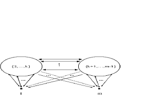
Figure 2: Graphical representation of the most general Partially Paired (PP) $m$-party graph. One circle contains parties $\{2,...,k\}$ and the other circle contains parties $\{k+1,...,m-1\}$. All parties within a circle can send and receive arrows from all other parties within the same circle. Each party in a circle can send and receive arrows to all parties in the other circle. Party 1 can send and receives arrows from parties $\{2,...,k\}$. Party 1 can receive arrows from (but does not send arrows to) parties $\{k+1,...,m-1\}$. Party $m$ can receive and send arrows to parties $\{k+1,...,m-1\}$. Party $m$ can receive arrows from (but does not send arrows to) parties $\{2,...,k\}$. There are no arrows between parties 1 and $m$. With these restrictions there is no party that receives arrows both from party 1 and party $m$. The subgraph composed only of the arrows emanating from parties 1 and $m$ is therefore separable. The graph thus belongs to the PP class.

By contrast, graphs in which, for any given pair of settings, there is always a party with results dependent on that pair (such as Fig. 1iv a,b)), can represent extreme points which reach the maximum value of $S_{4}$, namely $4$. It is straightforward to show that the graph of Fig. 1iva) with $a_{1}(x_{1},x_{2},x_{3},x_{4})$ can represent a function $\vec{a}(\vec{x})$ which will obtain the algebraic maximum. The graph in Fig. 1ivb), despite having apparently less communication than iii), also has extremal points which reach this maximum. Recalling, for graph ivb) that, $a_{1}(x_{1},\wedge,x_{3},\wedge),a_{3}(\wedge,x_{2},x_{3},x_{4}),$ $a_{2}(x_{1},x_{2},\wedge,\wedge),a_{4}(x_{1},x_{2},\wedge,x_{4})$, (8) becomes:

$$\frac{1}{4}\Big{[}-(-1)^{a_{1}(0,\wedge,0,\wedge)+a_{2}(0,0,\wedge\wedge)+a_{3}(\wedge,0,0,0)+a_{4}(0,0,\wedge,0)}$$

$$+(-1)^{a_{1}(0,\wedge,0,\wedge)+a_{2}(0,0,\wedge,\wedge)+a_{3}(\wedge,0,0,1)+a_{4}(0,0,\wedge,1)}$$

$$+(-1)^{a_{1}(0,\wedge,1,\wedge)+a_{2}(0,0,\wedge,\wedge)+a_{3}(\wedge,0,1,0)+a_{4}(0,0,\wedge,0)}$$

$$+(-1)^{a_{1}(0,\wedge,1,\wedge)+a_{2}(0,0,\wedge,\wedge)+a_{3}(\wedge,0,1,1)+a_{4}(0,0,\wedge,1)}\Big{]}$$ (12)

If we set $a_{3}(\wedge,0,1,0)=a_{4}(0,0,\wedge,0)=1$ and all of the other terms above equal to zero the expression takes value $1$. It is relatively easy, to find, by inspection a set of $a_{i}$ such that $S_{4}$ reaches its algebraic maximum of $4$. Indeed defining $a_{1}(x_{1},x_{3})=x_{1}x_{3}+x_{1};\;\;a_{2}(x_{1},x_{2})=x_{1}x_{2}+x_{2};\;\;a_{3}(x_{2},x_{3},x_{4})=x_{2}x_{3}+x_{3}x_{4}+x_{3};\;\;a_{4}(x_{1},x_{2},x_{4})=x_{1}x_{4}+x_{2}x_{4}+x_{4}+1$ obtains the maximum value for $S_{4}$. In this case it may be seen that:

$$\sum^{4}_{i=1}a_{i}(\vec{x})=\sum_{i<j}^{4}x_{i}x_{j}+\sum_{i=1}^{4}x_{i}+1.$$ (13)

This form will prove significant later.

A deterministic strategy with functional form represented by Fig. 1iii) is non-local: it can be pictured as requiring faster than light correlations. Nonetheless it cannot always replicate quantum statistics as we have described above. Conversely, as we described, extremal points represented by graphs like iva,b) can reach the algebraic maximum of $S_{4}$, namely 4.

Note that individual extremal points represented by graphs like iva,b) are signalling: by looking at the outputs of one party one can learn about the inputs of other parties. We will show below, however, that there exist convex combinations of extremal points represented by graphs like iva,b) which are no-signalling and which reach the algebraic maximum of $S_{4}$. This is an important remark since special relativity only permits no-signalling correlations.

Before moving to the $m$-party generalisation, we review: we have identified two kinds of four party correlations. The first are correlations represented by graphs i)-iii) and the second represented only by graphs like iv). The former reach a value of $\langle S_{4}\rangle\leq 2$ the later can reach $S_{4}=4$. For all quantum states $\langle S_{4}\rangle\leq 2\sqrt{2}$.

VI The $m$-party Svetlichny Polynomial

Having sketched proofs for the four-party Svetlichny polynomial, $S_{4}$, we can provide general proofs for the $m$-party setting with polynomials $S_{m}$. We first recall the definition of $S_{m}$, as formulated in Col .

We again consider the situation where each party’s input $x_{i}\in\{0,1\}$ is a single bit and each party’s output $a_{i}\in\{0,1\}$ is a single bit. We will use the notation introduced at the beginning of section IV. As in Col we construct $S_{m}$ from the Mermin polynomials. (The Mermin inequality is just one of the correlation inequalities described in Wolf ; Zuk where all correlation inequalities for $n$ parties, each having 2 inputs and 2 outputs, were characterised). Let the two party Mermin polynomial be

$$M_{2}=\frac{1}{2}(A^{0}_{1}A^{0}_{2}+A^{1}_{1}A^{0}_{2}+A^{0}_{1}A^{1}_{2}-A^{1}_{1}A^{1}_{2}),$$ (14)

and define the new notation:

$$M_{m}\equiv\sum_{\vec{x}}F_{m}(\vec{x})A_{1}^{x_{1}}A_{2}^{x_{2}}...A_{m}^{x_{m}},$$ (15)

where $\vec{x}=(x_{1},...,x_{m})$ and also

$$M^{\prime}_{m} \equiv \sum_{\vec{x}}F_{m}(\vec{x})A_{1}^{\overline{x}_{1}}A_{2}^{\overline{x}_{2}}...A_{m}^{\overline{x}_{m}}$$ (16)

$$= \sum_{\vec{x}}F_{m}(\vec{\overline{x}})A_{1}^{x_{1}}A_{2}^{x_{2}}...A_{m}^{x_{m}}$$

where $\overline{x}_{i}=x_{i}+1\mod 2$. $M_{m}$ is generated from $M_{m-1}$ by the recursion relation:

$$M_{m}=\frac{1}{2}\Big{[}M_{m-1}(A_{m}^{0}+A_{m}^{1})+M^{\prime}_{m-1}(A^{0}_{m}-A^{1}_{m})\Big{]}.$$ (17)

Using this twice yields:

$$M_{m+2}=\frac{1}{2}\Big{[}M_{m}(M_{2}+M^{\prime}_{2})+M^{\prime}_{m}(M_{2}-M^{\prime}_{2})\Big{]}.$$ (18)

The recursion relation (18) can be written in terms of $F_{m}$ as:

$$F_{m+2}(\vec{x})=$$

$$\quad\quad\frac{1}{2}\bigg{[}F_{m}(\vec{x})\Big{(}F_{2}(x_{m+1},x_{m+2})+F_{2}(\overline{x}_{m+1},\overline{x}_{m+2})\Big{)}$$

$$\quad\quad+F_{m}(\vec{\overline{x}})\Big{(}F_{2}(x_{m+1},x_{m+2})-F_{2}(\overline{x}_{m+1},\overline{x}_{m+2})\Big{)}\bigg{]}\ .$$

(19)

Following Col we define the Svetlichny polynomials as

$$S_{m}=\begin{cases}M_{m},&\text{if $m$ is even},\\ \frac{1}{2}(M_{m}+M^{\prime}_{m}),&\text{if $m$ is odd}.\end{cases}$$ (20)

We also define

$$S_{m}=\sum_{\vec{x}}\mu_{m}(\vec{x})A^{x_{1}}_{1}...A_{m}^{x_{m}},$$ (21)

which implies:

$$\mu_{m}(\vec{x})=\begin{cases}F_{m}(\vec{x}),&\text{if $m$ is even}\\ \frac{1}{2}\Big{[}F_{m}(\vec{x})+F_{m}({\vec{\overline{x}}})\Big{]},&\text{if $m$ is odd}.\end{cases}$$ (22)

In order to have a useful characterisation of $S_{m}$ we will obtain an explicit expression for $\mu_{m}$ and $F_{m}$:

Lemma 1 Let $q=\lceil m/2\rceil$ (where $\lceil\rceil$ indicates rounding up to the next nearest integer). Then

$$\mu_{m}(\vec{x})=\frac{1}{2^{q}}(-1)^{\left[\sum^{m}_{i<j}x_{i}x_{j}+(q+1)\sum_{i=1}^{m}x_{i}+(q^{2}-q)/2\right]},$$ (23)

and:

$$F_{2k+1}(\vec{x})=\frac{1}{2}F_{2k}(x_{1},\ldots,x_{2k})\left(1+(-1)^{\sum_{i=1}^{2k}x_{i}+x_{2k+1}+k}\right)\ .$$ (24)

As an example, note that in the four party, case one finds:

$$\mu_{4}(\vec{x})=\frac{1}{4}(-1)^{\left[\sum_{i<j}^{4}x_{i}x_{j}+\sum_{i=1}^{4}x_{i}+1\right]},$$ (25)

which (combined with (21)) reproduces eq. (6). Note that the exponent in (25) is identical to (13).

We now turn to the proof of Lemma 1.

Proof of Lemma 1.

Proof of Eq. (23) for m=2k, k integer.

In this case $\mu_{{2k}}=F_{{2k}}$. One easily checks that Lemma 1 is true for $k=1$ when

$$F_{2}(x_{1},x_{2}) = \frac{1}{2}(-1)^{x_{1}x_{2}},$$

$$F_{2}(\overline{x}_{1},\overline{x}_{2}) = \frac{1}{2}(-1)^{x_{1}x_{2}+x_{1}+x_{2}+1}\ .$$

We now proceed by induction. We suppose Lemma 1 is true for $k$ and will show it is true for $k+1$. From eq. (23):

$$F_{2k}(\vec{\overline{x}})=\frac{1}{2^{k}}(-1)^{[\sum^{2k}_{i<j}(x_{i}+1)(x_{j}+1)+(k+1)\sum_{i=1}^{2k}(x_{i}+1)+(k^{2}-k)/2]}$$ (26)

where $F_{2k}(\vec{x})=F_{2k}(x_{1},...,x_{2k})$ and $q=k$. Eq. (26) can be written as:

$$F_{2k}(\vec{\overline{x}})=\frac{1}{2^{k}}(-1)^{[\sum^{2k}_{i<j}x_{i}x_{j}+k\sum_{i=1}^{2k}x_{i}+(k^{2}+k)/2]},$$ (27)

using the identities

$$\sum_{i<j}^{2k}\overline{x}_{i}\overline{x}_{j}=\sum_{i<j}^{2k}x_{i}x_{j}+\sum_{i}^{2k}x_{i}+k\;\;\text{ mod}\;\;2,$$ (28)

and $(-1)^{2\alpha}=1$, $(-1)^{-\alpha}=(-1)^{\alpha}$ for $\alpha$ integer. Inserting $F_{2}(x_{2k+1},x_{2k+2})$, $F_{2}(\overline{x}_{2k+1},\overline{x}_{2k+2})$, $F_{2k}(\vec{\overline{x}})$, $F_{2k}(\vec{x})$ into (19) and noting that,

$$F_{2k}(\vec{x})=(-1)^{\sum^{2k}_{i=1}x_{i}+k}F_{2k}(\vec{\overline{x}}),$$ (29)

the righthand side of (19) becomes:

$$F_{2k+2}(\vec{x})=\frac{1}{4}F_{2k}(\vec{\overline{x}})(-1)^{x_{2k+1}x_{2k+2}}(1+(-1)^{x_{2k+1}+x_{2k+2}}$$

$$+(-1)^{\sum_{i=1}^{2k}x_{i}+k}+(-1)^{x_{{2k}+1}+x_{{2k}+2}+\sum_{i=1}^{2k}x_{i}+k+1})$$

$$=\frac{1}{2}F_{2k}(\vec{\overline{x}})(-1)^{(x_{{2k}+1}+x_{{2k}+2})(\sum_{i=1}^{2k}x_{i}+k)+x_{{2k}+1}x_{{2k}+2}},$$ (30)

where we have used the identity:

$$(-1)^{(ab)}=\frac{1}{2}(1+(-1)^{b}+(-1)^{a}+(-1)^{a+b+1}),$$ (31)

for $a,b$ integer. Eq. (30) can be rewritten as:

$$F_{{2k}+2}(\vec{x})=\frac{1}{2^{k+1}}(-1)^{\sum_{i<j}^{2k}x_{i}x_{j}+(x_{{2k}+1}+x_{{2k}+2})(\sum_{i=1}^{2k}x_{i})}\times$$

$$(-1)^{x_{{2k}+1}x_{{2k}+2}+(k+2)\sum_{i=1}^{2k}x_{i}+(k+2)(x_{{2k}+1}+x_{{2k}+2})+(k^{2}+k)/2}.$$

One can readily check that this coincides with Eq. (23) for $m=2k+2,\;\;q=k+1$. Eq. (23) thus satisfies the recursion relation (19) for ${2k}$ even. $\Box$

Proof of Eq. (24).

Eq. (17) can be rewritten as:

$$M_{{2k}+1}= \frac{1}{2}\Big{[}M_{2k}\sum^{1}_{x_{{2k}+1}=0}A^{x_{2k}+1}_{{2k}+1}$$ (33)

$$+M^{\prime}_{2k}\sum_{x_{{2k}+1}=0}^{1}(-1)^{x_{{2k}+1}}A^{x_{{2k}+1}}_{{2k}+1}\Big{]}.$$

Using (15), this is equivalent to the relation:

$$F_{{2k}+1}(\vec{x})=\frac{1}{2}\Big{[}F_{2k}(\vec{x})+F_{2k}(\vec{\overline{x}})(-1)^{x_{{2k}+1}}\Big{]}.$$ (34)

Substituting eq. (29) into eq. (34) one recovers eq. (24). $\Box$

Proof of Eq. (23) for m=2k+1, k integer.

Inserting equations (34) and (29) into eq. (22), for $m$ odd, yields:

$$\mu_{{2k}+1}(\vec{x})=\frac{1}{4}F_{2k}(\vec{\overline{x}})(1+(-1)^{\sum_{i=1}^{2k}(x_{i}+1)+x_{2k}+k+1}+$$

$$(-1)^{\sum^{2k}_{i=1}x_{i}+k}(1+(-1)^{\sum^{2k}_{i=1}x_{i}+k+x_{{2k}+1}})).$$ (35)

This becomes, by identity (31),

$$\mu_{{2k}+1}(\vec{x})=\frac{1}{2}F_{{2k}}(\vec{\overline{x}})(-1)^{x_{{2k}+1}(\sum^{{2k}}_{i=1}x_{i}+k)}.$$ (36)

This can be rewritten as:

$$\mu_{{2k}+1}(\vec{x})= \frac{1}{2^{k+1}}(-1)^{\sum_{i<j}^{2k}x_{i}x_{j}+x_{{2k}+1}\sum^{2k}_{i=1}x_{i}}\times$$ (37)

$$(-1)^{(k+2)(\sum_{i=1}^{2k}x_{i}+x_{{2k}+1})+(k^{2}+k)/2}$$

which coincides with (23). $\Box$

VII The Classes PP and TP

The central result of this article is to obtain bounds on the maximum value of $S_{m}$ attainable in different models. Let us recall what is already known in this respect:

Theorem 1:

[SS2002Seev ],[CGPRS2002Col ],[MPR2002Pop ]

1. Local hidden variable models and separable models satisfy the Svetlichny inequality

   $$\langle S_{m}\rangle_{\text{lhv, separable models}}\leq 2^{m-\lceil m/2\rceil-1}\ .$$ (38)

2. The maximum value of $S_{m}$ attainable by quantum mechanics (reached by carrying out measurements on the GHZ state) is

   $$\langle S_{m}\rangle_{\text{quantum mechanics}}\leq 2^{m-\lceil m/2\rceil-1/2}\ .$$ (39)

3. The algebraic maximum of $S_{m}$ (obtained by taking $A_{1}^{x_{1}}...A_{m}^{x_{m}}=\mu(\vec{x}_{m})/|\mu(\vec{x}_{m})|$ and using eq. (23)) is

   $$S_{m}[alg]=2^{m-\lceil m/2\rceil}\ .$$ (40)

We now go back to the classification of extreme points in terms of communication patterns introduced in section III. We define two classes of graph and formulate two theorems about them.

Definition 1: Partially Paired (PP) Graphs (see Fig. 2). A communication pattern represented by a directed graph in which there exist two (or more) parties $i,j$ such that there is no party with results dependent on $x_{i},x_{j}$. Graphically, this definition can be rephrased as: Take the subgraph composed only of the vertices receiving arrows originating from $i$ and $j$ and the arrows originating from $i$ and $j$. This graph is separable: it can be split into two disconnected graphs one including vertex $i$ and the other $j$.

Examples are Fig. 1i-iii) since, in these graphs, there is always a pair of vertices $i,j$ that neither send arrows to each other, nor both send to the same party.

Definition 2: Partially Paired Correlations. These are the correlations that can be written as convex combinations of the extremal correlations whose associated graph is partially paired. These correlations form the set $C_{PP}$:

$$C_{PP}=\cup_{G\in PP}C_{G}$$

(where PP is the set of all PP graphs). Note that $C_{PP}$ is the space of correlations associated with all possible PP graphs, not just a single PP graph $G_{PP}$.

One of our main results is:

Theorem 2. All Partially Paired correlations (ie. all correlations in the set $C_{PP}$) satisfy the multi-party Svetlichny inequality $S_{m}\leq 2^{m-q-1}$.

Note that the Svetlichny inequality is violated by some quantum states, see Theorem 1. Thus PP correlations cannot reproduce all quantum correlations.

The complementary class to PP graphs are the Totally Paired graphs:

Definition 3: Totally Paired (TP) Graphs. Any graph which is not $PP$. Graphically this can be rephrased as: for any two parties $i,j$ there always exists a party $k$ such that $k$ receives arrows originating from $i$ and $j$ ($k$ could coincide with $i$ or $j$).

Examples are Fig. 1iv,v) (see Gutin04 for a graph theoretic analysis of TP graphs).

The definition of TP graphs will allow us to prove the complement of Theorem 2. Namely we will show that for any TP graph $G_{TP}$, there exist correlations whose associated graph is $G_{TP}$ and which maximally violate the Svetlichny inequality.

But it should be noted that - except in the case of lhv models - an extreme point is a deterministic signalling strategy: one party’s results provides information about the settings of other parties. Thus one could argue that such extreme points are unphysical and cannot reproduce the predictions of causal theories, such as quantum mechanics, which do not allow signalling. But we will show that different strategies, with the same associated graph $G_{TP}$, can be combined to produce no-signalling correlations while continuing to maximally violate the Svetlichny inequality. Thus maximal violation of the Svetlichny inequality by correlations in $C_{G_{TP}}$, where $G_{TP}$ is an arbitrary $TP$ graph, is compatible with causality. These results are summarized in:

Theorem 3. For any Totally Paired communication graph $G_{TP}$, there exist correlations in the set $C_{G_{TP}}$ (the set of correlations obtained by convex combinations of the extremal points $E_{G_{TP}}$ whose associated graph is $G_{TP}$) which both attain the algebraic maximum of the Svetlichny polynomial and are no-signalling.

Note that $C_{G_{TP}}$ is the set of correlations associated with a single TP graph, $G_{TP}$.

Proof of Theorem 2

The Svetlichny inequalities can be written in the form

$$\langle S_{m}\rangle=\sum_{\vec{x},\vec{a}}\mu_{m}(\vec{x})(-1)^{\sum_{i}a_{i}}P(\vec{a}|\vec{x})\leq 2^{m-q-1}\ .$$ (41)

In the class $PP$ there always exists at least one pair of settings, say $x_{1},x_{m}$, such that no party’s outcome is dependent on both. As in Fig. 2, the $m$ parties can be divided into the set $\{1,...,k\}$ dependent on $x_{1}$ (and not $x_{m}$) and $\{k+1,...,m\}$ dependent on $x_{m}$ (and not $x_{1}$). Defining $\sum_{i=1}^{k}a_{i}\mod 2\equiv\beta_{1}$, $\sum_{i=k+1}^{m}a_{i}\mod 2\equiv\beta_{2}$, and rewriting the left hand side of (41) using (23):

$$\langle S_{m}\rangle_{PP}=\quad\quad\quad$$

$$\frac{1}{2^{q}}\sum_{x_{2},...,x_{m-1}}(-1)^{\sum_{i<j,i\neq 1}^{m-1}x_{i}x_{j}+(q+1)\sum^{m-1}_{i=2}x_{i}+(q^{2}-q)/2}$$

$$\times\bigg{(}\sum_{x_{1},x_{m},\vec{a}}(-1)^{x_{1}x_{m}+(q+1+\sum_{i=2}^{m-1}x_{i})(x_{1}+x_{m})}$$

$$\times(-1)^{\beta_{1}+\beta_{2}}P(\vec{a}|\vec{x})\bigg{)}$$ (42)

By the definition of $\beta_{1},\beta_{2}$,

$$\sum_{x_{1},x_{m},\vec{a}}(-1)^{x_{1}x_{m}+(q+1+\sum_{i=2}^{m-1}x_{i})(x_{1}+x_{m})}(-1)^{\beta_{1}+\beta_{2}}P(\vec{a}|\vec{x}),$$ (43)

has the same form as a $CHSH$ expression CHSH and thus has a modulus $\leq 2$. Substituting this into (42) yields $\langle S_{m}\rangle_{PP}\leq 2^{m-q-1}$. $\Box$

Thus, at least insofar as the Svetlichny inequality is concerned, the set $C_{PP}$ is only as strong as its subset, the separable correlations considered in Seev ; Col .

Proof of Theorem 3.

Any extreme point in the set of correlations, ie. any deterministic scenario, has $\vec{a}=\vec{a}(\vec{x})$ and so (41) becomes

$$\langle S_{m}\rangle=\sum_{\vec{x}}\mu_{m}(\vec{x})(-1)^{\sum_{i}a_{i}(\vec{x})}$$ (44)

In order to reach the algebraic maximum of $S_{m}$ we require $(-1)^{\sum_{i}a_{i}(\vec{x})}=\mu(\vec{x})/|\mu(\vec{x})|$. From Lemma 1, this means that the algebraic maximum is attained if

$$\sum^{m}_{i=1}a_{i}=\sum^{m}_{i<j}x_{i}x_{j}+(q+1)\sum_{i=1}^{m}x_{i}+(q^{2}-q)/2.$$ (45)

Let us show that for any Totally Paired graph $G_{TP}$, there is an extreme point whose associated graph is $G_{TP}$ and which satisfies eq. (45). To see this note the following:

1. $a_{i}(\vec{x})$ is a function of $x_{j}$ only when there is an arrow originating at vertex $j$ and ending at vertex $i$. (In addition $a_{i}$ can always depend on $x_{i}$).

2. For any pair of vertices $i,j$ in a $TP$ graph there is always a vertex $k$ which either receives edges from both members of the pair or is itself a member of the pair (ie. $k$ can coincide with either $i$ or $j$). The output of this vertex $a_{k}(\vec{x})$ can thus be equal to any function of $x_{i}$ and $x_{j}$ (Plus possibly other functions depending on the other arrows leading into vertex $k$). By an appropriate choice of these functions we can reproduce the term $\sum_{i<j}^{m}x_{i}x_{j}$ on the right hand side of eq. (45).

3. The output of any vertex $i$ can depend on the input to vertex $i$. Hence the output of vertex $i$ can contain a term equal to $a_{i}(x_{i})=cx_{i}+d$. By combining these terms we can reproduce the term $(q+1)\sum_{i=1}^{m}x_{i}+(q^{2}-q)/2$.

By combining points 2 and 3 above, we can satisfy eq. (45).

Thus certain extreme points in $E_{G_{TP}}$ (where $G_{TP}$ is any $TP$ graph) define functions $\vec{a}(\vec{x})$ such that (45) holds. These reach the algebraic maximum of the multi-party Svetlichny polynomials. Convex combinations of these will also obtain the maximum. This is why (13) has the same form as the exponent of (25).

We now turn to the second part of Theorem 3. We will show that different strategies, with the same associated graph, $G_{TP}$, can be combined to produce no-signalling correlations while continuing to maximally violate the Svetlichny inequality. Let us first recall that by no-signalling correlations we mean correlations $P(\vec{a}|\vec{x})$ such that one subset of parties, say parties $1,\ldots,k$, cannot communicate to the other parties $k+1,\ldots,m$ by changing the settings of their measurement device. Mathematically this is expressed by the condition that for all $a_{k+1},\ldots,a_{m}$

$$\sum_{a_{1},\ldots,a_{k}}P(\vec{a}|\vec{x})=P(a_{k+1},\ldots,a_{m}|\vec{x})$$ (46)

where the right hand side is independent of $x_{1},\ldots,x_{k}$.

Let us now consider a particular graph $G_{TP}$ in the set $TP$. To this graph we can associate at least one deterministic strategy $\vec{a}\,^{0}(\vec{x})$ such that eq. (45) holds. This deterministic strategy is necessarily signalling, ie. eq. (46) is not independent of $x_{1},\ldots,x_{k}$. The first step in proving the second part of Theorem 3 is to note that $\vec{a}\,^{0}(\vec{x})$ is not the only deterministic strategy which has $G_{TP}$ as its associated graph and which obeys eq. (45). In fact from $\vec{a}\,^{0}(\vec{x})$ we can easily construct a set of $2^{m-1}$ deterministic strategies that all have $G_{TP}$ as their associated graph and obey eq. (45). To this end define the $m$ component vectors, $\vec{b}^{\mu}\in\{0,1\}^{m}$ with the property $\sum_{i}{b^{\mu}_{i}}\;\rm mod\;2=0$. There are $2^{m-1}$ such vectors, $\vec{b}^{1},\vec{b}^{2}...\vec{b}\,^{2^{m-1}}$. Now we define $\vec{a}^{\mu}(\vec{x})=\vec{a}\,^{0}(\vec{x})+\vec{b}^{\mu}$. Note that $\sum_{i}a^{\mu}_{i}\;\rm mod\;2$ =$\sum_{i}a^{0}_{i}\;\rm mod\;2$, hence eq. (45) holds for all deterministic strategies $\vec{a}^{\mu}(\vec{x})$.

The second step in proving the second part of Theorem 3 is to note that, while staying constrained by the graph $G_{TP}$, the parties need not use a deterministic strategy. Instead, before the protocol starts, they can choose one value of $\mu$ at random, according to some probability distribution $p(\mu)\geq 0$, $\sum_{\mu}p(\mu)=1$. They then carry out the deterministic strategy $\vec{a}^{\mu}(\vec{x})$. Since $\mu$ is chosen at random the resulting correlations have the form

$$P(\vec{a}|\vec{x})=\sum_{\mu}p(\mu)P^{\mu}(\vec{a}|\vec{x})$$ (47)

where $P^{\mu}(\vec{a}|\vec{x})$ are the correlations obtained by using the deterministic strategy $\vec{a}^{\mu}$. Thus the parties have formed a convex combination of deterministic strategies, all with the same associated graph $G_{TP}$.

Let us now show that if $p(\mu)=2^{-(m-1)}$ is the uniform distribution, then the correlations defined by eq. (47) are no-signalling. This follows from the fact that the correlations associated with $\vec{a}^{\mu}$ have the form $P^{\mu}(\vec{a}|\vec{x})=\delta\big{(}a_{1}-\small(a_{1}^{0}(\vec{x})+b^{\mu}_{1}\small)\big{)}\delta\big{(}a_{2}-\small(a_{2}^{0}(\vec{x})+b^{\mu}_{2}\small)\big{)}\ldots\delta\big{(}a_{m}-(a_{m}^{0}(\vec{x})+b^{\mu}_{m})\big{)}$. We can now show that $P(a_{k+1},\ldots,a_{m}|\vec{x})$ is independent of $x_{1},...x_{k}$:

$$P(a_{k+1},\ldots,a_{m}|\vec{x})=\frac{1}{2^{m-1}}\sum_{a_{1},\ldots,a_{k}}\sum_{\mu}P^{\mu}(\vec{a}|\vec{x})$$ (48)

$$= \!\!\!\!\frac{1}{2^{m-1}}\!\!\!\!\sum_{a_{1},...,a_{k}}\!\!\!\!\sum_{\;\;\mu}\delta\big{(}a_{1}\!\!-\!\!(a_{1}^{0}(\vec{x})+b^{\mu}_{1})\big{)}...\delta\big{(}a_{m}\!\!-\!\!(a_{m}^{0}(\vec{x})+b^{\mu}_{m})\big{)}$$

$$= \!\!\!\!\frac{1}{2^{m-1}}\sum_{\mu}\Big{(}\delta\big{(}a_{k+1}\!\!-\!\!(a_{k+1}^{0}(\vec{x})+b^{\mu}_{k+1})\big{)}...\delta\big{(}a_{m}\!\!-\!\!(a_{m}^{0}(\vec{x})+b^{\mu}_{m})\big{)}$$

$$\times\;\;\sum_{a_{1},\ldots,a_{k}}\delta\big{(}a_{1}\!\!-\!\!(a_{1}^{0}(\vec{x})+b^{\mu}_{1})\big{)}\ldots\delta\big{(}a_{k}\!\!-\!\!(a_{k}^{0}(\vec{x})+b^{\mu}_{k})\big{)}\Big{)}$$

$$= \!\!\!\!\frac{1}{2^{m-1}}\sum_{\mu}\delta\big{(}a_{k+1}\!\!-\!\!(a_{k+1}^{0}(\vec{x})\!\!+\!\!b^{\mu}_{k+1})\big{)}...\delta\big{(}a_{m}\!\!-\!\!(a_{m}^{0}(\vec{x})\!\!+\!\!\,b^{\mu}_{m})\big{)}$$

where we use the fact that

$$\sum_{a_{1},...,a_{k}}\delta\big{(}a_{1}-(a_{1}^{0}(\vec{x})+b_{1}^{\mu})\big{)}...\delta\big{(}a_{k}-(a_{k}^{0}(\vec{x})+b_{k}^{\mu})\big{)}=1$$ (49)

whatever the value of $\vec{a}\,^{0}(\vec{x})+\vec{b}^{\mu}$ and for all $\mu$, and $\vec{x}$. Now note that for any given $m-k$ element bit string, $(a_{k+1},...,a_{m})$, and $m-k$ element bit string, $(a^{0}_{k+1}(\vec{x}),...,a^{0}_{m}(\vec{x})\,)$ (for given $\vec{x}$), there are $2^{k-1}$ vectors $\vec{b}^{\mu}$ such that $(a_{k+1},...,a_{m})=(a^{0}_{k+1}(\vec{x}),...,a^{0}_{m}(\vec{x}))+(b^{\mu}_{k+1},...,b^{\mu}_{m})$. Thus, upon summing over $\mu$, one finds, from eq. (48), that $P(a_{k+1},\ldots,a_{m}|\vec{x})=2^{k-m}$ for all $a_{k+1},\ldots,a_{m}$ and for all $\vec{x}$. The result is true for any $1\leq k\leq m$. Thus no non-trivial subgroup of the parties can signal to any other. The correlations in eq. (47) are therefore non-signalling. $\Box$.

VIII Conclusion

Svetlichny Svet and then others Seev ; Col demonstrated that classical models which allow superluminal communication within subsets of parties cannot reproduce all multipartite quantum correlations. We have extended this approach and showed that much more general classical communication patterns than those considered in Seev ; Col cannot reproduce all multipartite quantum correlations. We have shown how to describe such communication patterns in terms of directed graphs. (For instance the correlations considered in Svet ; Seev ; Col are described by separable graphs). Our main result is to prove that correlations described by Partially Paired (PP) Graphs (see definition 1) cannot reproduce all quantum correlations. PP graphs are much more general than separable graphs, and therefore our result shows that, in the multipartite setting, quantum correlations are much more non-local than previously thought. To obtain this result we carried out a detailed analysis of the properties of the multiparty generalisation of the Svetlichny inequality for which the bounds attained by lhv models, quantum mechanics, and completely non-local models were previously known. We showed that the correlations associated with PP graphs attain the same bound as the lhv models, and therefore cannot reproduce all quantum correlations. While for purposes of exposition, we described the four party case in section V, it should be noted that there are three party non-separable PP correlations; for example $a_{1}(x_{1},x_{2},\wedge),a_{2}(x_{1},x_{2},\wedge),a_{3}(\wedge,x_{2},x_{3})$. In other words, the phenomenon we have described in this paper, namely that quantum mechanics is stronger than some in-separable correlations, appears even for three party states. We have also found that another class of correlations which are convex combinations of some of the extreme points associated with Totally Paired (TP) graphs (see definition 3) can both maximally violate the Svetlichny inequality and be no-signalling. However this does not necessarily mean that any TP graph has associated extreme points which can reproduce all multipartite quantum correlations. Indeed the above results give an essentially complete characterisation of how much different classical communication patterns violate the Svetlichny inequality. But there are many other Bell inequalities which can be used to probe the non-locality of quantum correlations. It may be that - using another Bell inequality as test - one can show that some TP graphs represent correlations that cannot reproduce all quantum correlations. On the other hand it may be that the extreme points associated with any TP graph can reproduce all quantum correlations. We leave this as an open question for future research. Indeed the present work shows that the non-locality present in multipartite quantum correlations is stronger, and structurally richer, than previously thought.

References

• (1) J.S. Bell, Physics 1, 195 (1964).
• (2) G. Brassard, R. Cleve, and A. Tapp, Phys. Rev. Lett. 83, 1874 (1999).
• (3) M. Steiner, Phys. Lett. A 270, 239 (2000).
• (4) S. Massar, D. Bacon, N. J. Cerf, and R. Cleve, Phys. Rev. A 63, 052305 (2001).
• (5) B. F. Toner and D. Bacon, Phys. Rev. Lett. 91, 187904 (2003).
• (6) G. Svetlichny, Phys. Rev. D 35, 3066 (1987).
• (7) M. Seevinck and G. Svetlichny, Phys. Rev. Lett. 89, 060401 (2002).
• (8) D. Collins, N. Gisin, S. Popescu, D. Roberts, and V. Scarani, Phys. Rev. Lett. 88, 170405 (2002).
• (9) R.F. Werner and M.M. Wolf, Phys. Rev. A 64, 032112 (2001).
• (10) M. Zukowski and C. Brukner, Phys. Rev. Lett. 88, 210401 (2002).
• (11) Effectively there are two hidden variables. In addition to $\lambda$, the variable $i\in\{1,2,3\}$ defines which pair in the triple can communicate
• (12) P. Mitchell, S. Popescu, and D. Roberts, Phys. Rev. A 70, 060202 (2004).
• (13) G. Gutin, N.S. Jones, A. Rafiey, S. Severini and A. Yeo, e-print math.CO/0411653 and in Discrete Applied Mathematics forthcoming.
• (14) J.F. Clauser, M.A. Horne, A. Shimony, and R.A. Holt, Phys. Rev. Lett. 23, 880 (1969).