Breakdown of an Electric-Field Driven System:
a Mapping to a Quantum Walk

Abstract

Quantum transport properties of electron systems driven by strong electric fields are studied by mapping the Landau-Zener transition dynamics to a quantum walk on a semi-infinite one-dimensional lattice with a reflecting boundary, where the sites correspond to energy levels and the boundary the ground state. Quantum interference induces a distribution localized around the ground state, and a delocalization transition occurs when the electric field is increased, which describes the dielectric breakdown in the original electron system.

Dynamics of quantum statistical systems driven by finite external fields has attracted much attention as a typical class of non-equilibrium phenomenon. One problem is the “dissipation” arising in electron systems driven out of their ground states by strong electric fields as studied by many authors Oka2003 ; Lenstra1986 ; Landauer1985 ; Gefan1987 ; Blatter1988 ; Cohen2000PRL ; Fishman1982 . In these references the electric field is expressed (via Faraday’s electro-magnetic induction) as a time-dependent Aharonov-Bohm(AB) flux, and this induces, for strong fields, interlevel Landau-Zener transitions. There, an issue is whether the bunch of energy levels around the one having the main amplitude can play a role akin to dissipationCohen2000PRL . The purpose of the present study is to propose a mapping of the system onto a quantum algorism model for studying the problem. We start by noting that the driven quantum system and the quantum algorism model have in fact similarities: The former deals with quantum transitions among macroscopic number of energy levels while the latter describes the dynamics of many qubits governed by quantum logic gates, for which powerful analytical techniques are being developed.

In the one-dimensional tight-binding model, the Hamiltonian is $H(\phi(t))=-t\sum_{i,\sigma}\left[e^{-i\frac{2\pi}{L}\phi(t)}c_{i+1\sigma}^{\dagger}c_{i\sigma}+\mbox{h.c.}\right]+\hat{V}$, where $c_{i,\sigma}^{\dagger}$ creates an electron at $i=1,2,\ldots L$ with spin $\sigma=\uparrow,\downarrow$, the AB-flux measured in units of the flux quantum $\phi(t)=FLt/h$ represents the electric field $F$, and $\hat{V}$ the external potential or electron-electron interaction. Disordered mesoscopic systemsLenstra1986 ; Landauer1985 ; Gefan1987 ; Blatter1988 have been treated with this Hamiltonian, which has been extended to a strongly correlated electron system by three of the present authorsOka2003 . The adiabatic energy levels against $\phi$ have many level anti-crossings (as schematically shown in Fig.1(a)), which come from the disorder in disordered (one-body) systems, or from Umklapp processes in correlated systems. The system obeys the time-dependent Schrödinger’s equation starting from the ground state $|\Psi_{0}\rangle$ of $H(0)$, where its formal solution is $\hat{T}e^{-i\int_{0}^{t}H(\phi(s))ds}|\Psi_{0}\rangle$. When the field is finite, non-adiabatic Landau-Zener tunneling processes occur at the level anti-crossings, which take place first from the ground state and then among higher excited states. Authors of Lenstra1986 ; Gefan1987 ; Blatter1988 introduced a transfer matrix representation to mimic the evolution $\hat{T}e^{-i\int_{0}^{t}H(\phi(s))ds}$, where a set of $2\times 2$ unitary matrices represent the transitions among neighboring energy levels. Extensive studies on this model have found the existence of a dynamical localizationFishman1982 , or an Anderson localization in energy spaceBlatter1988 . However, the effect of quantum interference, which should be the key to the Anderson localization, has been studied only numericallyLandauer1985 ; Lenstra1986 ; Gefan1987 ; Blatter1988 .

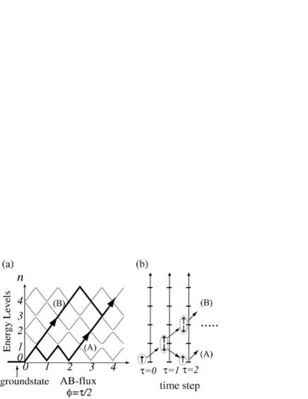
Figure 1: (a) Idealized energy levels of an electron system on a ring plotted against the AB-flux $\phi=FLt/h$, which increases linearly with time after the electric field $F$ is turned on at $t=0$. Two paths (A, B) for the Landau-Zener transition among neighboring levels are shown. (b) A mapping to a quantum-walk, where the energy levels are mapped to sites of the qubits and the ground state to a reflecting boundary.

Now we want to point out that the Landau-Zener transitions in multi-level systems presented above can be mapped to a quantum walk on a lattice. We shall show that the localization (in energy axis) of wave functions can be studied in terms of an exact solution for the transition amplitudes in the quantum walk. Quantum walk is a quantum counterpart of the random walkKempe2003 ; Tregenna2003 ; ChalkerCoddington ). The mapping we conceive here between the quantum walk and the Landau-Zener dynamics is straightforward: A qubit on site $n\geq 0$ labeled by $L,R$ corresponds to the states at the $n$-th anticrossing point, which moves down ($L$; with a left-going current) or up ($R$; right-going) in energy after the tunneling event(Fig.1). One important point we note here is that the mapped quantum walk has a reflecting boundary, since we cannot walk below the ground state in energy. In previous quantum-walk studiesBach2002absorption ; Yamasaki2003 ; Konno2003 an absorbing boundary was considered, for which the generating functions were obtainedKonno2003 . Here we first obtain the generating function for the quantum walk with a reflecting boundary. We have found the existence, and an analytic form for, the amplitude localized around the boundary (the ground state in the original problem). The solution exhibits an asymmetry between the L and R states, which represents a finite total momentum. When the electric field exceeds a critical value, a delocalization transition (on energy axis) is observed, which we identify here to describe the dielectric breakdown in the original electron model.

Mapping — Let the wave function for the $n$-th energy level at time $\tau$ (measured in units of $\Delta t/2=h/2FL$) be $\Psi(n,\tau)=\vspace{0cm}^{t}(\psi_{L}(n,\tau),\psi_{R}(n,\tau))$, where $\psi_{L}(n,\tau)(\psi_{R}(n,\tau))$ has a left- (right-) momentum. Each energy level is subject to a Landau-Zener tunneling (with certain probability and phase) to neighboring levels in a time period $\Delta t/2$. While transitions among more than three levels exist in principle, here we restrict ourselves to transitions among neighboring levels, for which the quantum tunneling can be described by a set of $2\times 2$ unitary matricesLenstra1986 ; Landauer1985 ; Gefan1987 ; Blatter1988 . The diagonal elements represent Landau-Zener tunneling, while the off-diagonal ones the backward scattering process. Here we simplify the problem by assuming that the matrices are the same $U=\left(\begin{array}[]{cc}a&b\\ c&d\end{array}\right)$ except for the one at the boundary, $\tilde{U}\equiv\left(\begin{array}[]{cc}\tilde{a}&\tilde{b}\\ \tilde{c}&\tilde{d}\end{array}\right).$ As we shall see, an interesting structure arises in the overall shape of the distribution in the bounded quantum walk even within this simplification.different The wave function evolves deterministically following a recursion formula,

$$\Psi(n,\tau+1)=P\Psi(n+1,\tau)+Q\Psi(n-1,\tau)$$ (1)

for excited ($n\geq 2$) states, while we put

$$\Psi(1,\tau+1) = P\Psi(2,\tau)+\tilde{Q}\Psi(0,\tau),$$

$$\Psi(0,\tau+1) = P\Psi(1,\tau)$$ (2)

between the ground and the first excited levels. Here we have decomposed $U$ into $P\equiv(^{ab}_{00})$, $Q\equiv(^{00}_{cd})$ and $\tilde{Q}\equiv(^{00}_{\tilde{c}\tilde{d}})$. Equations(1),(2) define the mapping to a one-dimensional quantum walk on a semi-infinite space with a reflecting boundary at $n=0$. We take the initial wave function $|\Psi_{0}\rangle$ to be the ground state, i.e., $\Psi(0,0)=\vspace{0cm}^{t}(1,0)$ and $\Psi(n,0)=0$ for $n\geq 1$.

Generating function for the quantum walk — Now we state our main result for the quantum walk: We can obtain the generating function for the wave function in the reflecting boundary condition, where the generating function is defined as $\Psi^{L,R}(0\to n;z)=\sum_{\tau=0}^{\infty}\psi_{L,R}(n,\tau)\;z^{\tau}$, with the summation taken over all the paths starting from $0$ and ending at $n$. The obtained expression is

$$\Psi^{L}(0\to n;z) = \left(\frac{d\lambda_{+}(z)}{a}\right)^{n-1}\frac{\tilde{c}d}{ac}\;\frac{\lambda_{+}(z)-az}{1-\tilde{c}A^{r}(0\to 0;z)},$$

$$\Psi^{R}(0\to n;z) = \left(\frac{d\lambda_{+}(z)}{a}\right)^{n-1}\frac{\tilde{c}z}{1-\tilde{c}A^{r}(0\to 0;z)},$$ (3)

$$\lambda_{+}(z)=\frac{\Delta z^{2}+1-\sqrt{\Delta^{2}z^{4}+2\Delta(1-2|a|^{2})z^{2}+1}}{2dz}.$$

Here $\Delta\equiv{\rm det}U=ad-bc$, and $A^{r}(0\to 0;z)=[d\lambda_{+}(z)-\Delta z]z/c$ is the generating function for the quantum walk with an absorbing boundary, governed by Eqs.(1,2) with ${\tilde{Q}}=0$Konno2003 .

In order to obtain the generating function (Breakdown of an Electric-Field Driven System: a Mapping to a Quantum Walk), we first express the transition amplitudes $\tilde{\Xi}^{b}(0\to n;\tau)$ as a sum of the contributions from paths starting from the $0$-th level (ground state) ending at the $n$-th level after $\tau$ steps. For example, $\tilde{\Xi}^{b}(0\to 2;4)=QPQ\tilde{Q}+PQ^{2}\tilde{Q}+Q\tilde{Q}P\tilde{Q}$ consists of three paths, where the quantum nature of the walk appears as the matrices being complex, i.e., different paths interfere with each other. The transition amplitude relates the initial vector $\Psi(0,0)$ to the wave function via $\Psi(n,\tau)=\tilde{\Xi}^{b}(0\to n;\tau)\Psi(0,0)$. We also introduce $\tilde{\Xi}^{a}(0\to n;\tau)$ as the transition amplitude in the quantum walk with an absorbing boundary; e.g., $\tilde{\Xi}^{a}(0\to 2;4)=QPQ\tilde{Q}+PQ^{2}\tilde{Q}$.

We obtain the transition amplitudes by employing a technique called the PQRS methodKonno2002a . Since the four matrices $P$, $Q$, $R\equiv(^{cd}_{00})$ and $S\equiv(^{00}_{ab})$, with ${\tilde{P}},\;{\tilde{Q}},\;{\tilde{R}},\;{\tilde{S}}$ defined similarly, span an orthonormal basis in $M_{2}(\mathbb{C})$ with an inner product $\langle A|B\rangle={\rm Tr}(A^{\dagger}B)$, we can express the transition amplitude $\tilde{\Xi}^{b}(0\to n;\tau)$ as a linear combination,

$$\tilde{\Xi}^{b}(0\to n;\tau)=\tilde{b}^{\tilde{q}}(0\to n;\tau)\tilde{Q}+\tilde{b}^{\tilde{r}}(0\to n;\tau)\tilde{R}$$ (4)

with the tilde basis, where ${\tilde{P}}$ and ${\tilde{S}}$ terms are absent. Thus, eq.(4) defines a set of complex numbers $\tilde{b}^{\tilde{q}}(0\to n;\tau)$ and $\tilde{b}^{\tilde{r}}(0\to n;\tau)$, and we denote ${\tilde{B}}^{{\tilde{q}},{\tilde{r}}}(0\to n;z)=\sum_{\tau=0}^{\infty}\tilde{b}^{{\tilde{q}},{\tilde{r}}}(0\to n;\tau)z^{\tau}$ as their generating functions. The generating functions ${\tilde{A}}^{{\tilde{q}},{\tilde{r}}}(0\to n;z)$ for the absorbing boundary problem is defined similarly from $\tilde{\Xi}^{a}(0\to n;\tau)=\tilde{a}^{\tilde{q}}(0\to n;\tau)\tilde{Q}+\tilde{a}^{\tilde{r}}(0\to n;\tau)\tilde{R}$. We note that for $n=0$ the $\tilde{Q}$ terms vanish, i.e., ${\tilde{B}}^{{\tilde{q}}}(0\to 0;z)={\tilde{A}}^{{\tilde{q}}}(0\to 0;z)=0$. For a special case $\tilde{U}=U$, we drop all the tilde marks $\Xi^{b}(0\to n;\tau),\;B^{q,r}(0\to n;z),\;b^{q,r}(0\to n;\tau)\ldots$.

The PQRS method establishes a connection between the generating functions via multiplication rulesKonno2002a for the $PQRS$ matrices. From a recursion relation between $\tilde{\Xi}^{b}(0\to 0;\tau)$ and $\Xi^{b}(0\to n-1;\tau-1)$, we obtain

$${\tilde{B}}^{\tilde{q}}(0\to n;z) = \left[1+{\tilde{c}}{\tilde{B}}^{\tilde{r}}(0\to 0;z)\right]dzB^{q}(0\to n-1;z),$$ (5)

$${\tilde{B}}^{\tilde{r}}(0\to n;z) = \left[1+{\tilde{c}}{\tilde{B}}^{\tilde{r}}(0\to 0;z)\right]dzB^{r}(0\to n-1;z).$$

With a repeated application of the no-tilde version of Eq.(5) we obtain $B^{q}(0\to n;z)=[d\lambda_{+}(z)/a]^{n}/d,\;B^{r}(0\to n;z)=[d\lambda_{+}(z)/a]^{n}[(\lambda_{+}(z)-az)/(acz)]$. Again using (5) with a relation between ${\tilde{B}}^{{\tilde{r}}}(0\to 0;z)$ and $A^{r}(0\to 0;z)$, we arrive at eqs.(Breakdown of an Electric-Field Driven System: a Mapping to a Quantum Walk) after a bit of algebra.

Edge states in energy space — One asset of the generating function is that we can show that there exist “edge states” in the bounded quantum walk. To actually show this let us take the Landau-Zener tunneling probability, $p=\exp(-\pi\overline{F}/F),$ where the Zener threshold electric field $\overline{F}\propto\Delta^{2}$ depends on the size of the gap $\Delta$Zener1934 ; Landau . We plug this in the transfer matrix,

$$U=\left(\begin{array}[]{cc}\sqrt{p}e^{i\beta}&\sqrt{1-p}e^{i\gamma}\\ -\sqrt{1-p}e^{-i\gamma}&\sqrt{p}e^{-i\beta}\end{array}\right),\;\tilde{U}=\left(\begin{array}[]{cc}0&e^{i\tilde{\gamma}}\\ -e^{-i\tilde{\gamma}}&0\end{array}\right),$$ (6)

where the diagonal elements of $\tilde{U}$ are set to zero to represent a complete reflection. The phases $\beta,\gamma,\tilde{\gamma}$ consist of the dynamical phase and the geometric phase (nonadiabatic counterpart to Berry’s phase). In physical systems (such as the Hubbard model) these phases at the level anti-crossings are generally nonzero (and depend on the driving force $F$).

Expanding the generating function (Breakdown of an Electric-Field Driven System: a Mapping to a Quantum Walk) into a power series in $z$ yields the time evolution of the wave function (Fig.2). We can see that $\Psi$ (distribution on energy axis) breaks up, after a transient period, into two parts, $\Psi(n,\tau)\sim\Psi_{\rm edge}(n,\tau)+\Psi_{\rm bulk}(n,\tau)$, where $\Psi_{\rm edge}$ is a component localized around the boundary (i.e., the ground state) while $\Psi_{\rm bulk}$ is a component traveling into the bulk (excited states) with a nearly constant velocity. Interestingly, the edge state only appears when the phase difference,

$$\theta\equiv\gamma-\tilde{\gamma},$$

between the bulk and boundary transfer matrices is nonzero (as is the case with physical systems as mentioned).

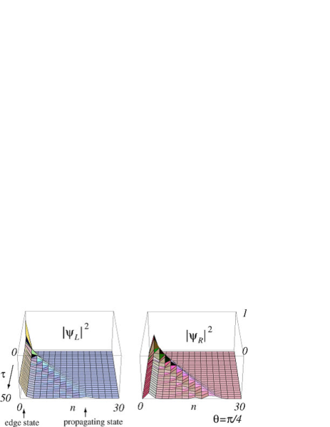
Figure 2: Time evolution of $|\psi_{L,R}(n,\tau)|^{2}$ with the initial condition $\psi_{L}(0,0)=1$. Here we set $p=0.2<p_{c}={\rm sin}^{2}\theta$, and only the amplitudes at even $n$ are displayed.

What is the nature of the edge state? The two generating functions $\Psi^{L,R}_{(0\to n)}(z)$ (eqs.(Breakdown of an Electric-Field Driven System: a Mapping to a Quantum Walk)) have a common, first-order pole in $z^{2}$ at $z_{\rm pole}^{2}=\frac{1-e^{-i\theta}\sqrt{1-p}}{1-e^{i\theta}\sqrt{1-p}}$. We can then obtain, with the Darboux’s methodDarboux , the asymptotic wave function, $\Psi_{\rm edge}(n,\tau)\to\exp\left({-i\epsilon\tau\Delta t/2\hbar}\right)\Phi_{\rm edge}(n),$ which obeys Floquet’s theoremFloquetReview with the Floquet mode $\Phi$ and the Floquet quasi-energy per length $\epsilon/L=(F/2\pi)\arg z_{\rm pole}^{2},$ a function of the electric field $F$ since $p=\exp(-\pi\overline{F}/F)$ involves $F$. We note that $\epsilon$ can be expressed as $\epsilon=-i\hbar\lim_{t\to\infty}\frac{1}{t}\ln\langle\Psi_{0}|U(t)|\Psi_{0}\rangle$, i.e., the asymptotic effective Hamiltonian of the system. An important observation here is that the elements of the Floquet state $\Phi_{\rm edge}(n)=\vspace{0cm}^{t}(\phi^{L}(n),\phi^{R}(n))$ with $\phi^{L,R}(n)=\lim_{z^{2}\to z^{2}_{\rm pole}}\Psi^{L,R}(0\to n;z)(1-z^{2}/z^{2}_{\rm pole})$, form a geometric series,

$$|\phi_{L}(n)|^{2} = r^{n}\;|\phi_{L}(0)|^{2},$$

$$|\phi_{R}(n\geq 2)|^{2} = r^{n-1}\;|\phi_{L}(0)|^{2},\quad n=0,2,\ldots,$$

$$r = p/(2-p-2\cos\theta\sqrt{1-p}),$$ (7)

with $|\phi_{L}(0)|^{2}=(1-r)^{2}$. Thus $\Phi(n)$ is an edge state exponentially localized (on energy axis) around the boundary $n=0$, whose weight is $|\Phi_{\rm edge}|^{2}=\sum_{n}(|\phi_{L}(n)|^{2}+|\phi_{R}(n)|^{2})=1-r$. The size (on energy axis) of the edge state is $\xi=1/|\ln r|,$ which behaves as $\xi\propto F/\overline{F}$ in the small $F$ regime and diverges like $\xi\propto\;|p-p_{c}(\theta)|^{-1}\propto\overline{F}|F-F_{c}(\theta)|^{-1}$ in the vicinity of the threshold, $p_{c}(\theta)=\sin^{2}\theta,F_{c}(\theta)=-\pi\overline{F}/(2\ln\sin\theta$). When $p$ exceeds $p_{c}(\theta)$, the edge state collapses, and only the component propagating into the bulk remains.

Translation to electron systems — Having presented the results for the quantum walk, we are now in position to translate them back to the electron system. The electric field $F$ causes a production of electron-hole pairs through the Landau-Zener tunneling. However, these excited charges cannot be accelerated indefinitely, since the electron-electron interaction or disorder scatter the momenta due to the “back scattering” at the level anti-crossings. This leads to bifurcations of the amplitude in energy space (whose example is depicted in Fig.1(a)). When different paths meet, quantum interference induces localization of the wave function, and the edge state $|\phi_{L,R}(n)|^{2}$, occurring for $\theta\neq 0$, in the quantum walk problem represents an effect of such an interference. So the present result is an analytic version of the edge states observed numerically in the long-time limitFishman1982 ; Gefan1987 ; Blatter1988 .

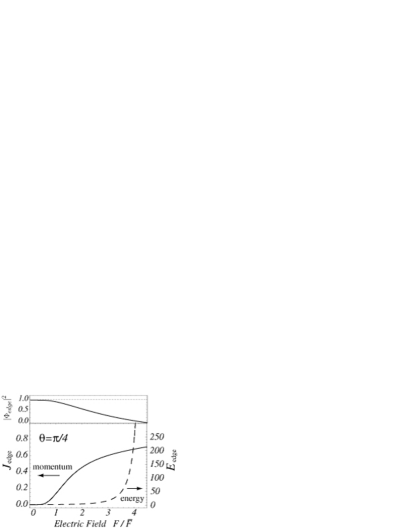
Figure 3: Total momentum $J_{\rm edge}$ and energy $E_{\rm edge}$ contributed by the edge component (eq.(8)) against the electric field $F$ for $\theta=\pi/4$. The upper figure depicts the weight of the edge state.

The momentum and energy expectation values (summed over L and R states) for the edge state are

$$J_{\rm edge} = \sum_{n}\left[j^{R}_{n}|\phi_{R}(n)|^{2}+j^{L}_{n}|\phi_{L}(n)|^{2}\right]/|\Phi_{\rm edge}|^{2},$$

$$E_{\rm edge} = \sum_{n}\left[E^{R}_{n}|\phi_{R}(n)|^{2}+E^{L}_{n}|\phi_{L}(n)|^{2}\right]/|\Phi_{\rm edge}|^{2}.$$ (8)

Here we normalize them by the total amplitude of the edge state $|\Phi_{\rm edge}(n)|^{2}$, which decreases as we increase the electric field and becomes zero at $F=F_{c}(\theta)$ (top panel of Fig.3). Following Lenstra1986 ; Landauer1985 ; Gefan1987 ; Blatter1988 , we choose $j^{R,L}_{n}=\pm j_{0}n,\;E^{R,L}_{n}=E_{0}n^{2},\;n=0,2,\ldots$ as the momentum and energy of the states, respectively, where $j_{0},\;E_{0}$ are units of momentum and energy. We note that the momentum measures the chiral asymmetry (between $L$ and $R$) of the distribution. By plugging in eq.(Breakdown of an Electric-Field Driven System: a Mapping to a Quantum Walk) we obtain $J_{\rm edge}=j_{0}\frac{p(2-p-2\cos\theta\sqrt{1-p})}{2\sqrt{1-p}(\sqrt{1-p}\cos\theta-1)^{2}}$, and a similar expression for $E_{\rm edge}$, valid for $F<F_{c}(\theta)$ (Fig.3). In the weak-field regime, the $J_{\rm edge}$ is suppressed until the Landau-Zener tunneling is activated for $F>\overline{F}$ when $J_{\rm edge}\propto\exp(-\pi\overline{F}/F)$ starts to rise. When $F$ is further increased to reach $F=F_{c}(\theta)$, the electric-field induced breakdown occurs, which corresponds, in the present picture, to the edge-to-propagating transition in the quantum walk. At the breakdown point the energy expectation value diverges as $E_{\rm edge}\sim|F-F_{c}(\theta)|^{-2}$. The $J_{\rm edge}$, however, does not diverge but shows a smooth increase.

Discussions — The idea of mapping the non-equilibrium problem to a quantum walk may apply to wider range of systems having many energy gaps. Here we have concentrated on the “edge state” when there is randomness (i.e., $\theta\neq 0$) only at the edge. Randomness in the transfer matrices in the excited state, ignored here, is expected to enhance the localization to bring $|\Phi_{edge}|^{2}$ closer to unity. Blatter et.alBlatter1988 have in fact obtained the expectation value of the momentum in such a situation, where the result resembles $J_{edge}$ obtained here. However, Blatter et.al did not obtain, in the range of electric field $F$ they have studied, a delocalization transition. In fact, Cohen et.al, in a random matrix model, found a disappearance of localized states in strong external fieldsCohen2000PRL . If such transitions also occur in electron systems, the quantum-walk picture may be used in understanding the transition. Indeed, some of the quantum-walk models now under study exhibit localization (e.g., Inui2004multi ), and the present mapping may shed lights on the non-equilibrium properties of driven quantum systems.

It is a pleasure to acknowledge V. Kagalovsky, Y. Matsuo, S. Miyashita, N. Nagaosa, and Y. Tokura for fruitful discussions in the early stage of the present work. We also wish to thank M. Katori and T. Sasamoto who suggested a link between the Landau-Zener transition and quantum walks. One of us (TO) thanks the Yukawa Institute for Theoretical Physics at Kyoto University, where this work was initiated during the YITP-W-03-18 on “Stochastic models in statistical mechanics”. Part of this work was supported by a JSPS fellowship for Young Scientists.

^∗ Present address: Max-Planck-Institut für Festkörperforschung, Stuttgart, D-70569 Germany

References

- (1) D. Lenstra and W. van Haeringen, Phys. Rev. Lett. 57, 1623 (1986).
- (2) R. Landauer, Phys. Rev. B 33, 6497 (1985).
- (3) Y. Gefen and D. J. Thouless, Phys. Rev. Lett. 59, 1752 (1987).
- (4) G. Blatter and D.A. Browne, Phys. Rev. B 37, 3856 (1988).
- (5) T. Oka, R. Arita, and H. Aoki, Phys. Rev. Lett. 91, 66406 (2003).
- (6) D. Cohen and T. Kottos, Phys. Rev. Lett. 85, 4839 (2000).
- (7) S. Fishman, D.R. Grempel, and R.E. Prange, Phys. Rev. Lett. 49, 509 (1982).
- (8) When the evolution matrix (including the phase ) differs from one level crossing to another, we can still use eq.(5) to recursively obtain the generating functions, which will be discussed in a separate publication.
- (9) J. Kempe, Contemporary Physics 44, 307 (2003).
- (10) B. Tregenna, et al., New J. Physics 5, 83 (2003).
- (11) A similar model has been employed to analyze the critical behavior of the integer quantum Hall system by J.T. Chalker and P.D. Coddington, J. Phys. C 21, 2665 (1988).
- (12) E. Bach et al., quant-ph/0207008.
- (13) T. Yamasaki, H. Kobayashi, and H. Imai, Phys. Rev. A 68, 012302 (2003).
- (14) N. Konno et al., J. Phys. A: Math. Gen. 36, 241 (2003).
- (15) N. Konno, Quantum Information Processing 1, 345 (2002).
- (16) C. Zener, Proc. Roy. Soc. A 145, 523 (1934).
- (17) L.D. Landau, Phys. Z. Sowjetunion 2, 46 (1932).
- (18) Darboux’s method states that, if can be expressed as with a non-singular function , then the then the asymptote become .
- (19) see e.g. P.Hänggi in T. Dittrich et al., Quantum Transport and Dissipation, Chap.5 (WILEY-VCH, 1998).
- (20) N. Inui and N. Konno, quant-ph/0403153.