Polarization squeezing in vertical-cavity surface-emitting lasers

Abstract

We further elaborate the theory of quantum fluctuations in vertical-cavity surface-emitting lasers (VCSELs), developed in Ref. Hermier02 . In particular, we introduce the quantum Stokes parameters to describe the quantum self- and cross-correlations between two polarization components of the electromagnetic field generated by this type of lasers. We calculate analytically the fluctuation spectra of these parameters and discuss experiments in which they can be measured. We demonstrate that in certain situations VCSELs can exhibit polarization squeezing over some range of spectral frequencies. This polarization squeezing has its origin in sub-Poissonian pumping statistics of the active laser medium.

I Introduction

In the last years there has been an increasing interest to the polarization properties of the vertical-cavity surface-emitting lasers (VCSELs). This interest is motivated in the first line by the potential applications of this type of lasers in the high-rate optical communications Schnitzer99 . But there is also more fundamental reason for understanding of the polarization behavior in VCSELs, namely, a possibility of generating the intensity-squeezed light using the sub-Poissonian pumping of the active medium Golubev ; Yamamoto86 . To date, squeezing in VCSELs has been demonstrated experimentally for both single-mode operation and in a multi-transverse-mode regime Degen ; Hermiera . In single-mode operation with only one linearly polarized mode above threshold the fluctuations in a sub-threshold mode with polarization orthogonal to the lasing mode can present large intensity noise vanExter ; Willemsen and, moreover, be highly correlated with the intensity fluctuations of the oscillating mode. This phenomenon can result in deterioration of squeezing observed in experiments with polarization sensitive optical elements. Therefore, polarization dynamics in VCSELs plays an important role for correct description of their quantum fluctuations.

At present, the standard theory that accounts for dynamics of two polarization components of the electromagnetic field in VCSELs is the so-called “spin-flip” model developed by San Miguel, Feng and Moloney SanMiguel . On the basis of this model several authors have formulated semiclassical theories of light fluctuations in VCSELs vanExter ; Willemsen ; vanExter98 ; vanExter99 ; Mulet01 . However, semiclassical description is inappropriate for intensity-squeezed light and, therefore, calls for fully quantum model of quantum fluctuations in VCSELs. The “quantum spin-flip” model was developed recently in Ref. Hermier02 . This model takes into account, on the one side, the dynamics of two polarization components of the electromagnetic field and, on the other side, the pumping statistics of the active laser medium. In particular, the quantum spin-flip theory allows for sub-Poissonian pumping statistics in which case VCSELs can generate the intensity-squeezed light.

In this paper we further elaborate the quantum spin-flip model of VCSELs, developed in Hermier02 . In particular, we apply the quantum Stokes parameters to describe the quantum self- and cross-correlations of two polarization components of the electromagnetic field generated by VCSELs. We analytically calculate the fluctuation spectra of the quantum Stokes parameters and discuss experiments in which they can be measured. We demonstrate that for the sub-Poissonian pumping statistics VCSELs can exhibit polarization squeezing in some range of spectral frequencies.

The paper is organized as follows. In Sec. II we give a short resume of the quantum spin-flip model developed in Ref. Hermier02 , and calculate analytically the spectral densities of quantum fluctuations of the quadrature components. In Sec. III we introduce the quantum Stokes parameters, their fluctuation spectra, and discuss the experiments where these fluctuations spectra can be measured. Using the results obtained in Sec. II we analytically calculate the fluctuation spectra of the quantum Stokes parameters. In Sec. IV with help of the analytical results obtained in Sec. III we illustrate graphically the possibilities of observation of polarization squeezing in VCSELs. We also provide the figures of typical cross-correlations spectra of photocurrents and cross-correlation spectra of the Stokes parameters $S_{2}$ and $S_{3}$ that can be measured experimentally. In Sec. V we summarize the results.

II Quantum spin-flip theory of VCSELs

II.1 Resume of the model

In this section we shall give a brief resume of the quantum spin-flip model of VCSELs developed in Ref. Hermier02 . We shall define the physical parameters of this model and provide the equations which will be used in the following sections. For more details we refer the reader to Ref. Hermier02 .

The semiclassical four-level spin-flip model of VCSELs was developed by San Miguel, Feng and Moloney SanMiguel . This model describes very well the dynamics of these semiconductor lasers and is widely used for understanding of such phenomena, for example, as polarization switching. The spin-flip model takes into account the spin sublevels of the total angular momentum of the heavy holes in the valence band and of the electrons in the conduction band. These four sublevels interact with two circularly polarized electromagnetic waves in the laser resonator and it is this interaction that is responsible for the complicated polarization dynamics manifested by this type of lasers.

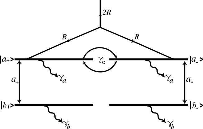
Figure 1: Four-level scheme of the active medium of VCSEL.

The four-level scheme of the semiconductor medium is shown in Fig. 1. Two lower levels $|b\pm\rangle$ correspond to the unexcited state of the semiconductor medium with zero electron-hole pairs while the upper levels $|a\pm\rangle$ to the excited states with an electron-hole pair created Koch . Two pairs of levels $|a+\rangle,|b+\rangle$ and $|a-\rangle,|b-\rangle$ are coupled via interaction with the left and right circularly polarized electromagnetic waves in the laser cavity described by the field operators $\hat{a}_{+}(t)$ and $\hat{a}_{-}(t)$. As explained in Ref. SanMiguel , physically these two pairs of transitions are associated with two $z$-components $J_{z}=\pm 1/2$ of the total angular momentum $J=1/2$ of the electrons in the conduction band and corresponding $z$-components $J_{z}=\pm 3/2$ for $J=3/2$ of the heavy holes in the valence band. The constants $\gamma_{a}$ and $\gamma_{b}$ are the decay rates of the populations of the upper and lower levels, $\gamma_{\perp}$ (not shown in Fig. 1) is the decay rate of the polarization, and $\gamma_{c}$ is the spin-flip rate that accounts for mixing of populations with opposite values of $J_{z}$. The last parameter was introduced in Ref. SanMiguel to describe the spin-flip relaxation process. This parameter is responsible for coupling of two transitions with different circular polarizations and, as a result, for various polarization dynamics of VCSELs.

It should be noted that the authors of Ref. SanMiguel have considered the situations of equal relaxation constants of the upper and the lower levels, $\gamma_{a}=\gamma_{b}$. However, it is known from the literature Golubev ; Yamamoto86 that this is not the most favorable condition for generation of the sub-Poissonian light. Therefore, the quantum spin-flip theory in Ref. Hermier02 was developed for arbitrary values of $\gamma_{a}$ and $\gamma_{b}$. In this paper we shall also consider this general situation.

Moreover, it has been mentioned in the literature (see, for example, Ref. Hermier02 ) that this model describes correctly a semiconductor laser if we assume the decay rate $\gamma_{b}$ of the lower levels to be very large compared to the other decay constants, namely, $\gamma_{a},\gamma_{c}$ and $\kappa$. From the classical point of view both situations $\gamma_{b}=\gamma_{a}$ and $\gamma_{b}\gg\gamma_{a}$ result in the same dynamical behavior of VCSELs. However, it turns out that the statistical properties of two models with $\gamma_{b}=\gamma_{a}$ and $\gamma_{b}\gg\gamma_{a}$ are very different. The detailed discussion of this difference is out of the scope of this paper and we shall address this point elsewhere.

We have indicated in Fig. 1 the pump process with mean total pumping rate $2R$ which is then separated with equal probabilities between two sublevels $|a_{+}\rangle$ and $|a_{-}\rangle$. Quantum spin-flip model of Ref. Hermier02 takes into account a possibility of sub-Poissonian pumping of the laser medium using the technique of the pump-noise suppression Golubev ; Yamamoto86 . For stationary in time average pumping rate, the influence of the pump statistics can be characterized by a single parameter $p\leq 1$ Benkert ; Kolobov . For $p=1$ the pump is perfectly regular while for $p=0$ the pump has Poissonian statistics. Intermediate values of $0\leq p\leq 1$ correspond to sub-Poissonian pumping while for $p\leq 0$ the pump process possess the excess classical fluctuations and corresponds to super-Poissonian statistics.

This pump statistics was introduced into the quantum spin-flip model using the Heisenberg-Langevin equations for the operator-valued collective populations ${\hat{N}}_{a\pm}(t)$, ${\hat{N}}_{b\pm}(t)$ of the upper and lower levels in Fig. 1, and for the collective polarization ${\hat{P}}_{\pm}(t)$. On the basis of the Heisenberg-Langevin equations, the equivalent $c$-number Langevin equations were derived for the collective atomic and field variables, corresponding to the normal ordering of the atomic and field operators Benkert ; Kolobov . Next, using the fact that the relaxation rates $\gamma_{b}$ of the lower levels and $\gamma_{\perp}$ of the polarization in VCSELs are much bigger than the relaxation rate $\gamma_{a}$ of the upper levels, the macroscopic $c$-number populations $N_{b\pm}(t)$ and the macroscopic $c$-number polarization $P_{\pm}(t)$ were adiabatically eliminated. The resulting equations can be written in terms of the total population of two upper levels $|a+\rangle$ and $|a-\rangle$, and of the total inversion between them. The corresponding variables are defined as $D(t)=(N_{a+}(t)+N_{a-}(t))/2$, and $d(t)=(N_{a+}(t)-N_{a-}(t))/2$. The equations for these variables and the two $c$-number field components $a_{\pm}(t)$ are

$$\dot{a}_{\pm}(t)=-\kappa a_{\pm}(t)-(\kappa_{a}+i\omega_{p})a_{\mp}(t)+c(1-i\alpha)\Bigl{[}D(t)\pm d(t)\Bigr{]}a_{\pm}(t)+F_{\pm}(t),$$ (1)

$$\dot{D}(t)=R-\gamma D(t)-c(|a_{+}(t)|^{2}+|a_{-}(t)|^{2})D(t)-c(|a_{+}(t)|^{2}-|a_{-}(t)|^{2})d(t)+F_{D}(t),$$ (2)

$$\dot{d}(t)=-\gamma_{s}d(t)-c(|a_{+}(t)|^{2}-|a_{-}(t)|^{2})D(t)-c(|a_{+}(t)|^{2}+|a_{-}(t)|^{2})d(t)+F_{d}(t).$$ (3)

Here $\kappa$ is the cavity damping constant, $\omega_{p}$ and $\kappa_{a}$ describe the linear birefringence and the linear dichroism of the semiconductor medium. The last parameter was not included into the model in Ref. Hermier02 and is introduced here as a generalization. Next, $\alpha$ is the linewidth enhancement in semiconductor lasers,

$$\alpha=\frac{\nu-\omega}{\gamma_{\perp}},$$ (4)

where $\nu$ is the frequency of the semiconductor energy gap, and $\omega$ is the resonator frequency. We have also defined the relaxation rate $\gamma_{s}$ as $\gamma_{s}=\gamma_{a}+2\gamma_{c}$, and have introduced the following shorthands,

$$c=\frac{g^{2}}{\gamma_{\perp}(1+\alpha^{2})},\hskip 14.22636pt\gamma=\gamma_{a},$$ (5)

where $g$ is the coupling constant of interaction of the electromagnetic field with the polarization.

The functions $F_{\pm}(t)$, $F_{D}(t)$ and $F_{d}(t)$ are the $c$-number Langevin forces. Their nonzero correlation functions were calculated in Ref. Hermier02 . In general the results are rather cumbersome but they are simplified in the vicinity of the stationary solutions. For completeness we shall give these correlation functions for the stationary solutions at the end of this section.

II.2 Stationary semiclassical solutions

Semiclassical equations of VCSELs are obtained from Eqs. (1)-(3) by dropping the $c$-number Langevin forces. In this subsection we shall give the stationary solutions of these equations which characterize the stationary generation of VCSELs. For investigation of quantum fluctuations in VCSELs we shall use standard assumption that these fluctuations are small compared to the corresponding stationary values. This will allow for linearization of Eqs. (1)-(3) around stationary solutions with respect to the quantum fluctuations.

Stationary solutions of Eqs. (1)-(3) have been investigated in detail in Martin-Regalado97 ; SanMiguel . When $\omega_{p}\neq 0$ and $\kappa_{a}\neq 0$ there are in general four types of stationary solutions: two of them have linear polarization along the $x$ and $y$ axes, and two other elliptical polarization. We shall consider only linearly polarized solutions because this type of solutions is usually realized in experiments. In this case the circularly polarized field components have equal amplitudes and can be written in the form

$$a_{\pm}(t)=Qe^{i(\Delta t\pm\psi)},$$ (6)

where the real amplitude $Q$ is normalized so that $Q^{2}=|a_{+}|^{2}=|a_{-}|^{2}$ gives the mean number of photons in the corresponding circularly polarized field mode. Two other parameters $\Delta$ and $\psi$ determine the type of polarization of the stationary solution (6).

We remind that the linearly polarized field components $a_{x}(t)$ and $a_{y}(t)$ are related to the circularly polarized ones as

$$a_{x}(t)=\frac{a_{+}(t)+a_{-}(t)}{\sqrt{2}},\quad a_{y}(t)=\frac{a_{+}(t)-a_{-}(t)}{\sqrt{2}i}.$$ (7)

For the $x$-polarized solution $\psi=0$ and for the $y$-polarized solution $\psi=\pi/2$. The frequency detunings $\Delta$ in Eq. (6) are different for these solutions and are equal to

$$\Delta_{x,y}=-[\kappa_{x,y}\alpha\pm\omega_{p}],$$ (8)

where the upper sign corresponds to the $x$-polarized solution and the lower sign to the $y$-polarized one. Here we have introduced the shorthands $\kappa_{x}=\kappa+\kappa_{a}$ and $\kappa_{y}=\kappa-\kappa_{a}$. The $x$-polarized stationary solution reads

$$a_{x}=\sqrt{2}Qe^{i\Delta_{x}t},\quad a_{y}=0,$$ (9)

while the $y$-polarized stationary solution is given by

$$a_{x}=0,\quad a_{y}=\sqrt{2}Qe^{i\Delta_{y}t}.$$ (10)

For both solutions we have

$$Q=\sqrt{I_{s}(r-1)},$$ (11)

where $r=R/R_{\rm th}$ is the dimensionless pumping rate, $R_{\rm th}$ is the threshold pumping rate, and $I_{s}$ is the saturation intensity; the two latter are given by

$$R_{\rm th}=\frac{\gamma\kappa_{x,y}}{c},\quad I_{s}=\frac{\gamma}{2c}.$$ (12)

Note that for $\kappa_{a}>0$ the threshold pumping rate for the $y$-polarized solution is lower that for the $x$-polarized one.

The stationary values of the atomic variables $d_{0}$ and $D_{0}$ for these linearly polarized solutions are equal to

$$d_{0}=0,\quad D_{0}=\frac{R}{\gamma+2cQ^{2}}=\frac{\kappa_{x,y}}{c}.$$ (13)

In the case of VCSELs as in general for solid-state and semiconductor lasers the question of stability of stationary solutions is very important. The stability analysis of these stationary solutions was performed in a number of publications, as for example, Refs. Martin-Regalado97 ; Golubev03 , and we refer the reader to this papers for details. In our analysis of quantum fluctuations we shall assume that the corresponding stationary operation regime of VCSEL is stable. Since for low pumping rate only $x$-polarized solution is stable, we shall restrict our analysis of quantum fluctuations only for this type of stationary solutions.

II.3 Linearization around stationary solutions

To calculate the quantum fluctuations around the stationary solution we shall linearize Eqs. (1)-(3) around the steady state given by Eq. (6). As mentioned above we shall consider here only $x$-polarized stationary solution. Adding small fluctuations to the stationary solutions we can write the field and the atomic variables as

$$a_{\pm}(t)=(Q+\delta a_{\pm}(t))e^{i\Delta t},\quad D(t)=D_{0}+\delta D(t),\quad d(t)=\delta d(t).$$ (14)

In this equation and in what follows we have dropped the index $x$ in $\Delta_{x}$ since we shall be concerned only with $x$-polarized solution. Substituting these expressions into Eqs. (1)-(3) and linearizing, we arrive at the following equations for small fluctuations,

$$\frac{d}{dt}\delta a_{\pm}(t) = (\kappa_{a}+i\omega_{p})\Bigl{(}\delta a_{\pm}(t)-\delta a_{\mp}(t)\Bigr{)}+c(1-i\alpha)Q(\delta D(t)\pm\delta d(t))+F_{\pm}(t)e^{-i\Delta t},$$

$$\frac{d}{dt}\delta D(t) = -\left(\gamma+2cQ^{2}\right)\delta D(t)-\kappa_{x}Q\left(\delta a_{+}(t)+\delta a_{-}(t)+c.c.\right)+F_{D}(t),$$

$$\frac{d}{dt}\delta d(t) = -\left(\gamma_{s}+2cQ^{2}\right)\delta d(t)-\kappa_{x}Q\left(\delta a_{+}(t)-\delta a_{-}(t)+c.c.\right)+F_{d}(t).$$ (15)

It is convenient to introduce the fluctuations of the linearly polarized components of the field $\delta a_{x}(t)$ and $\delta a_{y}(t)$, defined according to Eq. (7), for which the set of coupled equations (15) decouples in two sets of independent equations for $\delta a_{x}(t)$ and $\delta a_{y}(t)$ with Langevin forces $F_{x}(t)$ and $F_{y}(t)$ defined similar to Eq. (7). Moreover, we shall define the fluctuations of the amplitude and the phase quadrature components, $\delta X_{x}(t)$ and $\delta Y_{x}(t)$ of the $x$-polarized field component,

$$\delta X_{x}(t)=\frac{1}{2}\Bigl{(}\delta a_{x}(t)+\delta a_{x}^{\ast}(t)\Bigr{)},\quad\delta Y_{x}(t)=\frac{1}{2i}\Bigl{(}\delta a_{x}(t)-\delta a_{x}^{\ast}(t)\Bigr{)},$$ (16)

and similar for the $y$-polarized component. For these fluctuations we obtain the following equations,

$$\frac{d}{dt}\delta X_{x}(t) = \sqrt{2}cQ\delta D(t)+R_{x}(t),$$

$$\frac{d}{dt}\delta Y_{x}(t) = -\sqrt{2}\alpha cQ\delta D(t)+T_{x}(t),$$

$$\frac{d}{dt}\delta D(t) = -\Gamma\delta D(t)-2\sqrt{2}\kappa_{x}Q\delta X_{x}(t)+F_{D}(t),$$ (17)

and

$$\frac{d}{dt}\delta X_{y}(t) = 2\kappa_{a}\delta X_{y}(t)-2\omega_{p}\delta Y_{y}(t)-\sqrt{2}\alpha cQ\delta d(t)+R_{y}(t),$$

$$\frac{d}{dt}\delta Y_{y}(t) = 2\kappa_{a}\delta Y_{y}(t)+2\omega_{p}\delta X_{y}(t)-\sqrt{2}cQ\delta d(t)+T_{y}(t),$$

$$\frac{d}{dt}\delta d(t) = -\Gamma_{s}\delta d(t)+2\sqrt{2}\kappa_{x}Q\delta Y_{y}(t)+F_{d}(t),$$ (18)

where the new Langevin forces $R_{x}(t)$ and $S_{x}(t)$ are defined as

$$R_{x}(t) = \frac{1}{2}\Bigl{(}F_{x}(t)e^{-i\Delta t}+F_{x}^{\ast}(t)e^{i\Delta t}\Bigr{)},\quad T_{x}(t)=\frac{1}{2i}\Bigl{(}F_{x}(t)e^{-i\Delta t}-F_{x}^{\ast}(t)e^{i\Delta t}\Bigr{)},$$

$$R_{y}(t) = \frac{1}{2}\Bigl{(}F_{y}(t)e^{-i\Delta t}+F_{y}^{\ast}(t)e^{i\Delta t}\Bigr{)},\quad T_{y}(t)=\frac{1}{2i}\Bigl{(}F_{y}(t)e^{-i\Delta t}-F_{y}^{\ast}(t)e^{i\Delta t}\Bigr{)}.$$ (19)

In Eqs. (17) and (18) we have introduced

$$\Gamma\equiv\gamma+2cQ^{2}=\gamma r,\quad\Gamma_{s}\equiv\gamma_{s}+2cQ^{2}=\gamma_{s}+\gamma(r-1),$$ (20)

as convenient shorthands.

II.4 Spectral densities of quantum fluctuations

To solve Eqs. (17) and (18) we take the Fourier transform of the field and atomic fluctuations,

$$\delta X_{x}(\Omega)=\frac{1}{\sqrt{2\pi}}\int\limits_{-\infty}^{+\infty}\delta X_{x}(t)e^{i\Omega t}dt,$$ (21)

and similar for the other variables, that converts these differential equations into algebraic ones. The spectral correlation functions of these quadratures are $\delta$-correlated,

$$\langle\delta X_{i}(\Omega)\delta X_{i}(\Omega^{\prime})\rangle = (\delta X^{2}_{i})_{\Omega}\delta(\Omega+\Omega^{\prime}),$$

$$\langle\delta Y_{i}(\Omega)\delta Y_{i}(\Omega^{\prime})\rangle = (\delta Y^{2}_{i})_{\Omega}\delta(\Omega+\Omega^{\prime}),$$

$$\langle\delta X_{i}(\Omega)\delta Y_{i}(\Omega^{\prime})\rangle = (\delta X_{i}\delta Y_{i})_{\Omega}\delta(\Omega+\Omega^{\prime}),$$ (22)

with $(\delta X^{2}_{i})_{\Omega}$, $i=x,y$ and $(\delta Y^{2}_{i})_{\Omega}$ being the spectral densities of the corresponding quadratures, and $(\delta X_{i}\delta Y_{i})_{\Omega}$ their cross-spectral density.

After a simple algebra we obtain the following expressions for the fluctuations of the amplitude quadratures $\delta X_{x}(\Omega)$ and $\delta X_{y}(\Omega)$, and the phase quadrature $\delta Y_{y}(\Omega)$:

$$\delta X_{x}(\Omega)=\frac{1}{D_{x}(\Omega)}\Bigl{\{}(\Gamma-i\Omega)R_{x}(\Omega)+\sqrt{2}cQF_{D}(\Omega)\Bigr{\}},$$ (23)

$$\delta X_{y}(\Omega)=\frac{1}{D_{y}(\Omega)}\Bigl{\{}[2\kappa_{x}\gamma(r-1)-(2\kappa_{a}+i\Omega)(\Gamma_{s}-i\Omega)]R_{y}(\Omega)\Bigr{.}$$

. $$- [2\alpha\kappa_{x}\gamma(r-1)+2\omega_{p}(\Gamma_{s}-i\Omega)]T_{y}(\Omega)+\sqrt{2}cQ(2\omega_{p}+2\alpha\kappa_{a}+i\alpha\Omega)F_{d}(\Omega)\Bigr{\}},$$ (24)

$$\delta Y_{y}(\Omega) = \frac{1}{D_{y}(\Omega)}\Bigl{\{}2\omega_{p}(\Gamma_{s}-i\Omega)R_{y}(\Omega)\Bigr{.}$$

. $$- (2\kappa_{a}+i\Omega)(\Gamma_{s}-i\Omega)T_{y}(\Omega)+\sqrt{2}cQ(-2\alpha\omega_{p}+2\kappa_{a}+i\Omega)F_{d}(\Omega)\Bigr{\}},$$ (25)

with

$$D_{x}(\Omega) = -i\Omega(\Gamma-i\Omega)+2\kappa_{x}\gamma(r-1),$$

$$D_{y}(\Omega) = (\Gamma_{s}-i\Omega)[(2\omega_{p})^{2}+(2\kappa_{a}+i\Omega)^{2}]+2\kappa_{x}\gamma(r-1)(2\alpha\omega_{p}-2\kappa_{a}-i\Omega).$$ (26)

The other phase quadrature $\delta Y_{x}(\Omega)$ will not appear in the observables that we shall discuss below. Using the results obtained in Ref. Hermier02 and taking into account the stationary solutions (6) and (13) we obtain the following nonzero correlation functions of the Langevin forces $R_{i}(t),T_{i}(t)$ with $i=x,y$, and $F_{D}(t),F_{d}(t)$ for the stationary regime of VCSEL in approximation of the small fluctuations,

$$\langle R_{x}(t)R_{x}(t^{\prime})\rangle = \langle R_{y}(t)R_{y}(t^{\prime})\rangle=\langle T_{x}(t)T_{x}(t^{\prime})\rangle=\langle T_{y}(t)T_{y}(t^{\prime})\rangle=\kappa_{x}\delta(t-t^{\prime}),$$

$$\langle F_{D}(t)F_{D}(t^{\prime})\rangle = \frac{\kappa_{x}}{c}\Gamma\Bigl{(}1-\frac{1}{2}p\Bigr{)}\delta(t-t^{\prime}),$$

$$\langle F_{d}(t)F_{d}(t^{\prime})\rangle = \frac{\kappa_{x}}{c}\Gamma_{s}\delta(t-t^{\prime}),$$

$$\langle F_{D}(t)R_{x}(t^{\prime})\rangle = \langle F_{d}(t)T_{y}(t^{\prime})\rangle=-\sqrt{2}\kappa_{x}Q\delta(t-t^{\prime}).$$ (27)

Equations (23)-(26) together with correlation functions (27) allow us to evaluate an arbitrary correlation function of the laser light emitted by the VCSEL. The spectral densities of the amplitude quadratures $(\delta X_{x}^{2})_{\Omega}$, $(\delta X_{y}^{2})_{\Omega}$ are given by,

$$(\delta X_{x}^{2})_{\Omega}=\frac{\kappa_{x}}{|D_{x}(\Omega)|^{2}}\Bigl{\{}\Omega^{2}+\gamma^{2}r\Bigl{[}1-(r-1)p/2\Bigr{]}\Bigr{\}},$$ (28)

$$(\delta X_{y}^{2})_{\Omega}=\frac{\kappa_{x}}{2|D_{y}(\Omega)|^{2}}\Bigl{\{}\Omega^{4}+A_{X}\Omega^{2}+4B_{X}\Bigr{\}},$$ (29)

with $A_{X}$ and $B_{X}$ determined as,

$$A_{X} = \Bigl{[}2\kappa_{a}-\gamma(r-1)\Bigr{]}^{2}+\Bigl{[}2\omega_{p}+\alpha\gamma(r-1)\Bigr{]}^{2}-4\kappa\gamma(r-1)$$

$$+ \gamma_{s}\Bigl{[}\gamma_{s}+\gamma(r-1)(\alpha^{2}+2)\Bigr{]},$$

$$B_{X} = \Bigl{[}\kappa_{a}\gamma_{s}-\kappa\gamma(r-1)\Bigr{]}^{2}+\Bigl{[}\omega_{p}\gamma_{s}+\alpha\kappa\gamma(r-1)\Bigr{]}^{2}+\gamma_{s}\gamma(r-1)(\alpha\kappa_{a}+\omega_{p})^{2},$$ (30)

The spectral density of the phase quadrature component $(\delta Y_{y}^{2})_{\Omega}$ is equal to,

$$(\delta Y_{y}^{2})_{\Omega}=\frac{\kappa_{x}}{2|D_{y}(\Omega)|^{2}}\Bigl{\{}\Omega^{4}+A_{Y}\Omega^{2}+4B_{Y}\Bigr{\}},$$ (31)

with $A_{Y}$ and $B_{Y}$ given by,

$$A_{Y} = 4(\kappa_{a}^{2}+\omega_{p}^{2})+\gamma_{s}^{2}+\gamma(r-1)(4\alpha\omega_{p}+\gamma_{s}),$$

$$B_{Y} = \gamma_{s}^{2}(\kappa_{a}^{2}+\omega_{p}^{2})+\gamma_{s}\gamma(r-1)\Bigl{[}\omega_{p}^{2}(\alpha^{2}+2)+\kappa_{a}^{2}\Bigr{]}^{2}+\omega_{p}^{2}\gamma^{2}(r-1)^{2}(\alpha^{2}+1),$$ (32)

Finally the cross-spectral density $(\delta X_{y}\delta Y_{y})_{\Omega}$ reads,

$$(\delta X_{y}\delta Y_{y})_{\Omega}=\frac{-\kappa_{x}\gamma(r-1)}{2|D_{y}(\Omega)|^{2}}\Bigl{\{}\alpha\kappa_{x}\Omega^{2}+2\kappa\omega_{p}\gamma(r-1)(\alpha^{2}+1)+2\gamma_{s}\Bigl{[}\kappa(\alpha\kappa_{a}+\omega_{p})+\alpha\kappa_{a}(\kappa_{a}-\alpha\omega_{p})\Bigr{]}\Bigr{\}},$$ (33)

These analytical results will be used below for evaluation of the spectral densities of the quantum Stokes parameters, their cross-spectral densities and for the cross-correlation spectra of the photocurrents.

III Quantum polarization states of light: general discussion

III.1 Quantum Stokes parameters

There are two equivalent descriptions of the polarization properties of light in classical optics either by the polarization matrix or in terms of the classical Stokes parameters Born99 . During the last decade the quantum-mechanical version of the classical Stokes parameters was introduced in the literature and very actively used in quantum optics to describe the quantum fluctuations of polarization of the electromagnetic field Jauch76 ; Robson74 ; Chirkin93 ; Klyshko97 . There have been several theoretical proposals for generation of polarization-squeezed light Chirkin93 ; Korolkova94 ; Chirkin95 ; Alodjants95 ; Korolkova96 ; Korolkova02 and a few experiments in which such kind of light was observed  Grangier87 ; Karasev93 ; Buchev01 ; Bowen02 .

We shall use the language of the quantum Stokes parameters for characterization of the quantum fluctuations of polarized light in VCSELs. In this section we shall express the fluctuation spectra of the quantum Stokes parameters through the spectral densities of the quadrature components evaluated above. In the next section we shall apply these results for the particular case of VCSELs.

Let us write the operator $\vec{\hat{E}}(t)$ of the electromagnetic field at the output of the VCSEL in terms of the $x$- and $y$-polarized components,

$$\vec{\hat{E}}(t)=\hat{a}_{x}(t)\vec{e}_{x}+\hat{a}_{y}(t)\vec{e}_{y},$$ (34)

where $\hat{a}_{x}(t)$ and $\hat{a}_{y}(t)$ are the photon annihilation operators in the Heisenberg representation. In what follows we shall omit the time argument when this does not create ambiguities. The quantum Stokes operators $\hat{S}_{\mu},\mu=0,1,2,3$ are introduced similarly to their classical counterparts (see, for example Korolkova02 ),

$$\hat{S}_{0} = \hat{a}^{{\dagger}}_{x}\hat{a}_{x}+\hat{a}^{{\dagger}}_{y}\hat{a}_{y},$$

$$\hat{S}_{1} = \hat{a}^{{\dagger}}_{x}\hat{a}_{x}-\hat{a}^{{\dagger}}_{y}\hat{a}_{y},$$

$$\hat{S}_{2} = \hat{a}^{{\dagger}}_{x}\hat{a}_{y}+\hat{a}^{{\dagger}}_{y}\hat{a}_{x},$$

$$\hat{S}_{3} = i(\hat{a}^{{\dagger}}_{y}\hat{a}_{x}-\hat{a}^{{\dagger}}_{x}\hat{a}_{y}).$$ (35)

Using the commutation relations for the photon annihilation and creation operators,

$$[\hat{a}_{i},\hat{a}^{{\dagger}}_{j}]=\delta_{ij},\quad(i,j=x,y),$$ (36)

it is easy to verify that the operator $\hat{S}_{0}$ commutes with all the others,

$$[\hat{S}_{0},\hat{S}_{\mu}]=0,\quad(\mu=1,2,3),$$ (37)

and that the operators $\hat{S}_{1}$, $\hat{S}_{2}$ and $\hat{S}_{3}$ satisfy the commutation relations similar to the components of the angular-momentum operator,

$$[\hat{S}_{1},\hat{S}_{2}]=2i\hat{S_{3}},\quad[\hat{S}_{2},\hat{S}_{3}]=2i\hat{S_{1}},\quad[\hat{S}_{3},\hat{S}_{1}]=2i\hat{S_{2}}.$$ (38)

The noncommutativity of these three Stokes operators does not allow their simultaneous measurement in any real physical experiment. The mean values $\langle\hat{S}_{\mu}\rangle,\mu=1,2,3$ and the variances $\Delta S_{\mu}=\sqrt{\langle(\hat{S}_{\mu}-\langle\hat{S}_{\mu}\rangle)^{2}\rangle}$ are given by the uncertainty relations Jauch76 ,

$$\Delta S_{1}\Delta S_{2}\geq|\langle\hat{S_{3}}\rangle|,\quad\Delta S_{2}\Delta S_{3}\geq|\langle\hat{S_{1}}\rangle|,\quad\delta S_{3}\delta S_{1}\geq|\langle\hat{S_{2}}\rangle|.$$ (39)

When the $x$- and $y$-polarized components of the electromagnetic field are in coherent states $|\alpha_{x}\rangle$ and $|\alpha_{y}\rangle$ i. e.,

$$\hat{a}_{x}|\alpha_{x}\rangle=\alpha_{x}|\alpha_{x}\rangle,\qquad\hat{a}_{y}|\alpha_{y}\rangle=\alpha_{y}|\alpha_{y}\rangle,$$ (40)

one can speak about the coherent polarization state of the electromagnetic field. The mean values of the quantum Stokes parameters in this state are obtained by replacing $\hat{a}_{x}\to\alpha_{x}$ and $\hat{a}_{y}\to\alpha_{y}$ in Eq. (35). For example, for the first two parameters one obtains,

$$\langle\hat{S}_{0}\rangle=|\alpha_{x}|^{2}+|\alpha_{y}|^{2}=\langle\hat{n}_{x}\rangle+\langle\hat{n}_{y}\rangle=\langle\hat{n}\rangle,$$

$$\langle\hat{S}_{1}\rangle=|\alpha_{x}|^{2}-|\alpha_{y}|^{2}=\langle\hat{n}_{x}\rangle-\langle\hat{n}_{y}\rangle,$$ (41)

where $\langle\hat{n}\rangle$ is the mean total number of photons in the electromagnetic wave. The variances of all four quantum Stokes parameters in this case are equal and given by Korolkova02 ,

$$\Delta S_{\mu}^{2}=\langle\hat{n}_{x}\rangle+\langle\hat{n}_{y}\rangle=\langle\hat{n}\rangle,\qquad\mu=0,1,2,3.$$ (42)

This property of the coherent polarization state allows one to define a polarization squeezed state similar to the definition of a single-mode squeezed state. According to Chirkin93 one can speak about polarization squeezing if one of the four variances $\Delta S_{\mu}$ of the Stokes parameters becomes smaller than that in the coherent state, i. e.  $\Delta S_{\mu}^{2}<\langle\hat{n}\rangle$ for at least one $\mu$.

Classical Stokes parameters $S_{\mu},\mu=0,1,2,3$ (without hats) are obtained as the mean values of their quantum versions defined in Eq. (35), $S_{\mu}=\langle\hat{S}_{\mu}\rangle$. From the classical point of view, all polarization properties of light are completely described by these four parameters: $S_{0}$ determines the total beam intensity, while three other parameters characterize the polarization state of the light beam. This polarization state in classical optics is often represented in a Poincaré sphere with $S_{1}$, $S_{2}$ and $S_{3}$ forming its three orthogonal axes.

In quantum optics to completely characterize polarization properties of light in addition to the mean values $S_{\mu}$ of the quantum Stokes parameters one has to determine their variances $\Delta S_{\mu}$. In general all these variances can be different and one can speak of an uncertainty ellipsoid in the Stokes-Poincaré space Klyshko97 . In general case, when different Stokes components are correlated, there are three additional parameters which determine the orientation axes of this uncertainty ellipsoid.

While the general description is outside of the scope of our paper, we shall illustrate below graphically that in the case of VCSELs different quantum Stokes components $\hat{S}_{\mu}$ can have different variances $\Delta S_{\mu}$. The quantum fluctuations of polarization in VCSELs are therefore characterized by an uncertainty ellipsoid in the Stokes-Poincaré space.

III.2 Measurement of the classical Stokes parameters

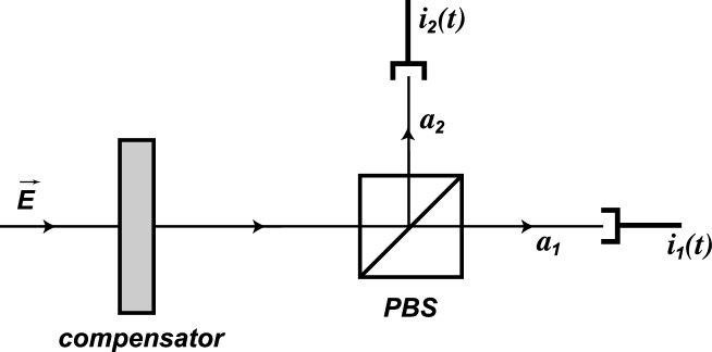
Figure 2: Experimental setup for measurement of the classical Stokes parameters.

Four classical Stokes parameters $S_{\mu}$ can be measured in an experimental setup shown in Fig. 2. This measurement scheme consists of a compensator, a polarizing beam splitter (PBS), and two photodetectors. Let $\delta_{x}$ and $\delta_{y}$ denote the phase changes produced by the compensator in the $x$- and $y$-components of the electromagnetic field given by Eq. (34). Next, let $\varphi$ denotes the angle between the transmission axis of the PBS and the $x$-axis. Then the field amplitudes $\hat{a}_{1}$ and $\hat{a}_{2}$ of the transmitted and reflected waves after the PBS can be written as

$$\hat{a}_{1} = e^{i\delta_{x}}(\hat{a}_{x}\cos{\varphi}+\hat{a}_{y}e^{-i\theta}\sin{\varphi}),$$

$$\hat{a}_{2} = e^{i\delta_{x}}(-\hat{a}_{x}\sin{\varphi}+\hat{a}_{y}e^{-i\theta}\cos{\varphi}),$$ (43)

where $\theta=\delta_{x}-\delta_{y}$ is the phase difference between the $x$- and $y$-components introduced by the compensator.

The secondary waves after PBS are photodetected and one observes the mean values of the photocurrents $\langle i_{1}\rangle=\eta c\langle\hat{a}^{{\dagger}}_{1}\hat{a}_{1}\rangle$, and $\langle i_{2}\rangle=\eta c\langle\hat{a}^{{\dagger}}_{2}\hat{a}_{2}\rangle$, where $\eta$ is the quantum efficiency of photodetection, and $c$ is the velocity of light (we have put the charge of electron equal to unity so that the photocurrents are measured in number of electrons per second). For simplicity in what follows we shall consider the situation of $\eta=1$. Using Eq. (43) we can write the mean photocurrent $\langle i_{1}\rangle$ measured in the transmission branch of the PBS as

$$\langle i_{1}\rangle\equiv\langle i_{1}(\varphi,\theta)\rangle=\frac{1}{2}\eta c\Bigl{[}S_{0}+S_{1}\cos{2\varphi}+(S_{2}\cos{\theta}+S_{3}\sin{\theta})\sin{2\varphi}\Bigr{]},$$ (44)

where $S_{\mu}$ are the classical Stokes parameters.

Equation (44) is the well-known formula for measuring the four classical Stokes parameters. The first three of them are obtained by removing the compensator $(\theta=0)$ and rotating the transmission axis of the PBS to the angles $\varphi=0^{\circ},45^{\circ}$, and $90^{\circ}$, respectively. The fourth parameter, $S_{3}$, is measured by using a compensator with $\theta=90^{\circ}$ or so-called quarter-wave plate, and setting the transmission axis of the PBS to $\varphi=45^{\circ}$. The four photocurrents are found to be, respectively,

$$\langle i_{1}(0^{\circ},0^{\circ})\rangle = \frac{1}{2}\eta c\left(S_{0}+S_{1}\right),$$

$$\langle i_{1}(45^{\circ},0^{\circ})\rangle = \frac{1}{2}\eta c\left(S_{0}+S_{2}\right),$$

$$\langle i_{1}(90^{\circ},0^{\circ})\rangle = \frac{1}{2}\eta c\left(S_{0}-S_{1}\right),$$

$$\langle i_{1}(45^{\circ},90^{\circ})\rangle = \frac{1}{2}\eta c\left(S_{0}+S_{3}\right).$$ (45)

Solving Eq. (45) for $S_{\mu}$ we can obtain all classical Stokes parameters from these four measurements.

III.3 Observation of the fluctuation spectra of the quantum Stokes parameters

In quantum optics in addition to the mean values of the quantum Stokes parameters $\langle\hat{S}_{\mu}\rangle$ their quantum fluctuations are also taken into account. In this paper to describe the quantum fluctuation we shall introduce the fluctuation spectra of the quantum Stokes parameters.

Let us split the quantum Stokes operators $\hat{S}_{\mu}(t)$ given by Eq. (35) into the stationary mean value $S_{\mu}=\langle\hat{S}_{\mu}\rangle$ and small fluctuation $\delta\hat{S}_{\mu}(t)$,

$$\hat{S}_{\mu}(t)=S_{\mu}+\delta\hat{S}_{\mu}(t).$$ (46)

Taking the Fourier transform of $\delta\hat{S}_{\mu}(t)$,

$$\delta\hat{S}_{\mu}(\Omega)=\frac{1}{\sqrt{2\pi}}\int\limits_{-\infty}^{+\infty}\delta\hat{S}_{\mu}(t)e^{i\Omega t}dt,$$ (47)

we can introduce the normally-ordered spectral correlation functions of the fluctuations $\delta\hat{S}_{\mu}(\Omega)$ similar to the spectral correlation functions of the quadrature components in Eq. (22), namely,

$$\langle:\delta\hat{S}_{\mu}(\Omega)\delta\hat{S}_{\mu}(\Omega^{\prime}):\rangle = (\delta S_{\mu}^{2})_{\Omega}\delta(\Omega+\Omega^{\prime}),$$

$$\langle:\delta\hat{S}_{\mu}(\Omega)\delta\hat{S}_{\nu}(\Omega^{\prime}):\rangle = (\delta S_{\mu}\delta S_{\nu})_{\Omega}\delta(\Omega+\Omega^{\prime}),\quad(\mu\neq\nu).$$ (48)

Here $(\delta S_{\mu}^{2})_{\Omega}$ are the spectral densities of the corresponding fluctuations and $(\delta S_{\mu}\delta S_{\nu})_{\Omega}$ their cross-spectral densities. The symbol $:\dots:$ means normal ordering of operators.

To measure the spectral densities $(\delta S_{\mu}^{2})_{\Omega}$ and the cross-spectral densities $(\delta S_{\mu}\delta S_{\nu})_{\Omega}$ of the quantum Stokes parameters given by Eq. (48) we can use an experimental setup similar to one that we have used for the measurement of the classical Stokes parameters (see Fig. 3). The difference is that instead of detecting the mean photocurrents $\langle i_{1}\rangle$ and $\langle i_{2}\rangle$ after the PBS, one observes now the photocurrent fluctuation spectra $(\delta i^{2}_{p})_{\Omega},p=1,2$ defined as

$$(\delta i^{2}_{p})_{\Omega}=\int\limits_{-\infty}^{+\infty}dt\;e^{i\Omega t}\langle\delta i_{p}(0)\delta i_{p}(t)\rangle,$$ (49)

where $\langle\delta i_{p}(0)\delta i_{p}(t)\rangle$ is the correlation function of the photocurrent fluctuations $\delta i_{p}(t)=i_{p}-\langle i_{p}\rangle$, and $\langle i_{p}\rangle$ is the mean value of the photocurrent. Alternatively, one can add and subtract the individual photocurrents in the secondary channels and to investigate the sum $i_{+}(t)=i_{1}(t)+i_{2}(t)$ and the difference $i_{-}(t)=i_{1}(t)-i_{2}(t)$ of two photocurrents. In this case the information about the fluctuation spectra of the quantum Stokes parameters is contained in the fluctuation spectra

$$(\delta i^{2}_{\pm})_{\Omega}=\int\limits_{-\infty}^{+\infty}dt\;e^{i\Omega t}\langle\delta i_{\pm}(0)\delta i_{\pm}(t)\rangle.$$ (50)

The photocurrent fluctuation spectra $(\delta i^{2}_{p})_{\Omega}$ and $(\delta i^{2}_{\pm})_{\Omega}$ can be easily expressed through the spectral densities $(\delta S^{2}_{\mu})_{\Omega}$ and the cross-spectral densities $(\delta S_{\mu}\delta S_{\nu})_{\Omega}$ of the four quantum Stokes parameters. The results are conveniently presented in terms of the following linear combination of the three Stokes operators, $\hat{S}_{1}$, $\hat{S}_{2}$, and $\hat{S}_{3}$,

$$\hat{S}=\hat{S}_{1}\cos{2\varphi}+(\hat{S}_{2}\cos{\theta}+\hat{S}_{3}\sin{\theta})\sin{2\varphi},$$ (51)

which is sometimes called a polarization observable Karasev93 ; Buchev01 . We obtain the following expressions for the fluctuation spectra $(\delta i^{2}_{p})_{\Omega}$ and $(\delta i^{2}_{\pm})_{\Omega}$, normalized to the shot-noise levels,

$$(\delta i^{2}_{1})_{\Omega}/\langle i_{1}\rangle = 1+\frac{\kappa}{2\langle n_{1}\rangle}\Bigl{[}(\delta S^{2}_{0})_{\Omega}+2(\delta S_{0}\delta S)_{\Omega}+(\delta S^{2})_{\Omega}\Bigr{]},$$ (52)

$$(\delta i^{2}_{2})_{\Omega}/\langle i_{2}\rangle = 1+\frac{\kappa}{2\langle n_{2}\rangle}\Bigl{[}(\delta S^{2}_{0})_{\Omega}-2(\delta S_{0}\delta S)_{\Omega}+(\delta S^{2})_{\Omega}\Bigr{]},$$ (53)

$$(\delta i^{2}_{-})_{\Omega}/\langle i_{+}\rangle = 1+\frac{2\kappa}{\langle n\rangle}(\delta S^{2})_{\Omega},$$ (54)

$$(\delta i^{2}_{+})_{\Omega}/\langle i_{+}\rangle = 1+\frac{2\kappa}{\langle n\rangle}(\delta S_{0}^{2})_{\Omega},$$ (55)

where the corresponding spectral densities and cross-spectral densities of are defined according to Eq. (48). Here $\langle i_{+}\rangle=\langle i_{1}\rangle+\langle i_{2}\rangle$ is the shot-noise level of the photocurrent sum and difference, $\langle n_{1}\rangle=\langle\hat{a}^{{\dagger}}_{1}\hat{a}_{1}\rangle$, and $\langle n_{2}\rangle=\langle\hat{a}^{{\dagger}}_{2}\hat{a}_{2}\rangle$ are the mean photon numbers in the corresponding secondary channels after the PBS, and $\langle n\rangle=\langle n_{1}\rangle+\langle n_{2}\rangle$.

Equations (52)-(55) are analogous of Eq. (44) for measuring the spectral densities of the quantum Stokes parameters. It is clear from these equations that with proper choice of angles $\theta$ and $\varphi$ all nonzero spectral densities and cross-spectral densities of the Stokes operators can be measured.

III.4 Relations between the spectral densities of the quantum Stokes parameters and of the quadrature components

In Sec. II D we have provided analytical results for the fluctuations of the quadrature components $\delta X_{x}(\Omega)$, $\delta X_{y}(\Omega)$, $\delta Y_{y}(\Omega)$, and for their spectral densities and cross-spectral densities [see Esq. (28)-(33)]. Now we shall express the spectral densities of the quantum Stokes operators through the spectral densities of these quadrature components. As before, we shall restrict ourselves to the case of the $x$-polarized stationary solution when $\langle n_{x}\rangle=2Q^{2}$ and $\langle n_{y}\rangle=0.$

Using the same normal rule of correspondence between the operators and their $c$-number representations as in Ref. Hermier02 we shall introduce the $c$-number variables $S_{\mu}(t)$ corresponding to the quantum Stokes operators $\hat{S}_{\mu}(t)$. Since in Eq. (35) the Stokes operators are normally ordered, the same relation holds true for $S_{\mu}(t)$ and the $c$-number variables $a_{i}(t)$ and $a^{\ast}_{i}(t)$, $i=x,y$.

Linearizing the $c$-number variables $S_{\mu}(t)$ around their stationary values $S_{\mu}$ as

$$S_{\mu}(t)=S_{\mu}+\delta S_{\mu}(t),$$ (56)

we can express the fluctuations $\delta S_{\mu}(t)$ through the fluctuations of the field components $\delta a_{x}(t)$ and $\delta a_{y}(t)$,

$$\delta S_{0}(t) = \delta S_{1}(t)=\sqrt{2}Q\Bigl{(}\delta a_{x}(t)+\delta a_{x}^{\ast}(t)\Bigr{)},$$

$$\delta S_{2}(t) = \sqrt{2}Q\Bigl{(}\delta a_{y}(t)+\delta a_{y}^{\ast}(t)\Bigr{)},$$

$$\delta S_{3}(t) = -\sqrt{2}iQ\Bigl{(}\delta a_{y}(t)-\delta a_{y}^{\ast}(t)\Bigr{)}.$$ (57)

Taking into account Eq. (16) we obtain the following results relating the spectral densities of the Stokes operators with those of the quadrature components,

$$(\delta S_{0}^{2})_{\Omega}=(\delta S_{1}^{2})_{\Omega} = 8Q^{2}(\delta X_{x}^{2})_{\Omega},$$

$$(\delta S_{2}^{2})_{\Omega} = 8Q^{2}(\delta X_{y}^{2})_{\Omega},$$

$$(\delta S_{3}^{2})_{\Omega} = 8Q^{2}(\delta Y_{y}^{2})_{\Omega},$$

$$(\delta S_{2}\delta S_{3})_{\Omega} = 8Q^{2}(\delta X_{y}\delta Y_{y})_{\Omega}.$$ (58)

With help of these relations we arrive at,

$$(\delta i^{2}_{1})_{\Omega}/\langle i_{1}\rangle = 1+8\kappa\Bigl{[}\cos^{2}{\varphi}(\delta X^{2}_{x})_{\Omega}+\sin^{2}{\varphi}(\delta X^{2}_{\theta})_{\Omega}\Bigr{]},$$ (59)

$$(\delta i^{2}_{2})_{\Omega}/\langle i_{2}\rangle = 1+8\kappa\Bigl{[}\sin^{2}{\varphi}(\delta X^{2}_{x})_{\Omega}+\cos^{2}{\varphi}(\delta X^{2}_{\theta})_{\Omega}\Bigr{]},$$ (60)

$$(\delta i^{2}_{-})_{\Omega}/\langle i_{+}\rangle = 1+8\kappa\Bigl{[}\cos^{2}{2\varphi}(\delta X^{2}_{x})_{\Omega}+\sin^{2}{2\varphi}(\delta X^{2}_{\theta})_{\Omega}\Bigr{]},$$ (61)

$$(\delta i^{2}_{+})_{\Omega}/\langle i_{+}\rangle = 1+8\kappa(\delta X^{2}_{x})_{\Omega}.$$ (62)

To simplify Eqs. (59)-(61) we have introduced the following shorthand notation,

$$\delta X_{\theta}(\Omega)=\cos{\theta}\;\delta X_{y}(\Omega)-\sin{\theta}\;\delta Y_{y}(\Omega),$$ (63)

with its spectral density $(\delta X^{2}_{\theta})_{\Omega}$ given by,

$$(\delta X^{2}_{\theta})_{\Omega}=\cos^{2}{\theta}(\delta X^{2}_{y})_{\Omega}-2\sin{\theta}\cos{\theta}(\delta X_{y}\delta Y_{y})_{\Omega}+\sin^{2}{\theta}(\delta Y^{2}_{y})_{\Omega}.$$ (64)

The mean values of the individual photocurrents $\langle i_{1}\rangle$ and $\langle i_{2}\rangle$, and of the photocurrent sum $\langle i_{+}\rangle=\langle i_{1}\rangle+\langle i_{2}\rangle$ are equal to

$$\langle i_{1}\rangle=2Q^{2}\kappa\cos^{2}{\varphi},\quad\langle i_{2}\rangle=2Q^{2}\kappa\sin^{2}{\varphi},\quad\langle i_{+}\rangle=2Q^{2}\kappa.$$ (65)

In the next section we shall investigate in detail the spectral densities of the quantum Stokes parameters and their cross-spectral densities.

IV Polarization states of light in VCSELs

IV.1 Polarization squeezing

The spectral densities $(\delta S_{\mu}^{2})_{\Omega}$ of the quantum Stokes parameters can be measured using any of three Eqs. (52)-(54). Here we shall use Eq. (54) corresponding to observation of the noise spectrum $(\delta i^{2}_{-})_{\Omega}(\varphi,\theta)$ of the photocurrent difference. With help of Eq. (51) we can bring the photocurrent noise spectrum $(\delta i^{2}_{-})_{\Omega}(\varphi,\theta)$ to the form

$$(\delta i^{2}_{-})_{\Omega}(\varphi,\theta)/\langle i_{+}\rangle = 1+\frac{2\kappa}{Q^{2}}\Bigl{\{}(\delta S_{1}^{2})_{\Omega}\cos^{2}{2\varphi}+\sin^{2}{2\varphi}\Bigl{[}(\delta S_{2}^{2})_{\Omega}\cos^{2}{\theta}$$ (66)

$$- (\delta S_{2}\delta S_{3})_{\Omega}\;2\sin{\theta}\cos{\theta}+(\delta S_{3}^{2})_{\Omega}\sin^{2}{\theta}\Bigr{]}\Bigr{\}}.$$

In this equation we have explicitly indicated the dependence of the observed noise spectrum on the angle $\theta$ introduced by the compensator and the angle $\varphi$ of the polarization beam splitter.

The spectral densities $(\delta S_{0}^{2})_{\Omega}=(\delta S_{1}^{2})_{\Omega}$ and $(\delta S_{2}^{2})_{\Omega}$ of the Stokes parameters $S_{0},S_{1}$ and $S_{2}$ are measured by removing the compensator $(\theta=0)$ and setting the transmission axis of the PBS to the angles $\varphi=0^{\circ}$ and $\varphi=45^{\circ}$. The spectral density of the parameter $S_{3}$ is obtained by using a compensator with $\theta=90^{\circ}$ (quarter-wave plate), and setting $\varphi=45^{\circ}$. The corresponding photocurrent fluctuation spectra are given by,

$$(\delta i^{2}_{-})_{\Omega}(0^{\circ},0^{\circ})/\langle i_{+}\rangle = 1+\frac{2\kappa}{Q^{2}}(\delta S_{1}^{2})_{\Omega},$$ (67)

$$(\delta i^{2}_{-})_{\Omega}(45^{\circ},0^{\circ})/\langle i_{+}\rangle = 1+\frac{2\kappa}{Q^{2}}(\delta S_{2}^{2})_{\Omega},$$ (68)

$$(\delta i^{2}_{-})_{\Omega}(45^{\circ},90^{\circ})/\langle i_{+}\rangle = 1+\frac{2\kappa}{Q^{2}}(\delta S_{3}^{2})_{\Omega},$$ (69)

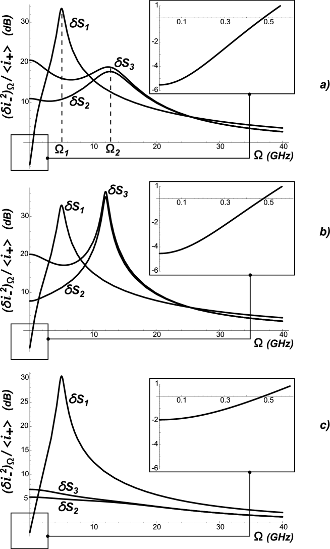
Figure 4: Photocurrent fluctuation spectra for the Stokes parameters $S_{1},S_{2}$ and $S_{3}$; a) without dichroism, $\kappa_{a}=0$, b) with dichroism, $\kappa_{a}=10\;GHz$, and c) with $\kappa_{a}=50\;GHz$. The values of other parameters are: $\kappa=100\;GHz$, $\gamma=1\;GHz$, $\gamma_{\perp}=1000\;GHz$, $\gamma_{s}=50\;GHz$, $\omega_{p}=40\;GHz$, $\alpha=3$ and $p=1$.

In Fig. 4 we have shown the photocurrent fluctuation spectra given by Eqs. (67)-(69) for physical parameters close to that used in experiment Hermier02 , namely, $\kappa=100\;GHz$, $\gamma=1\;GHz$, $\gamma_{\perp}=1000\;GHz$,$\gamma_{s}=50\;GHz$, $\omega_{p}=40\;GHz$, $\alpha=-3$, $r=6$, and $p=1$. The parameter $\kappa_{a}$, describing the dichroism of the laser crystal, was set equal to zero in Fig. 4a, to $\kappa_{a}=10\;GHz$ in Fig. 4b and to $\kappa_{a}=50\;GHz$ in Fig. 4c.

Let us first discuss the case without dichroism (Fig. 4a). As seen from Fig. 4a, the spectral density $(\delta S_{1}^{2})_{\Omega}$ of the Stokes parameter $S_{1}$ has a peak at a characteristic frequency $\Omega_{1}$, while two other spectra $(\delta S_{2}^{2})_{\Omega}$ and $(\delta S_{3}^{2})_{\Omega}$ for the Stokes parameters $S_{2}$ and $S_{3}$ exhibit peaks at another (higher) characteristic frequency $\Omega_{2}$. These peaks are well-known from the theory of solid-state and semiconductor lasers and have their physical origin in the relaxation oscillations due to a periodic energy exchange between the active medium and the laser radiation. Since in our case there are two upper levels $|a+\rangle$ and $|a-\rangle$ in the active laser medium, we have two subsystems where the periodic energy exchange takes place independently. First subsystem is described by the total population $D$ of the upper levels and the Stokes parameter $S_{1}$ [see Eqs. (17)], and its frequency of the relaxation oscillations is equal to $\Omega_{1}$. In the second subsystem the relaxation oscillations take place between the population difference $d$ and the two Stokes parameters $S_{2}$ and $S_{3}$ at the frequency $\Omega_{2}$ [see Eqs. (18)].

Second important feature that one can observe in Fig. 4a is reduction of the quantum fluctuations of the Stokes parameter $S_{1}$ below the standard quantum limit at low frequencies $\Omega$ in the case of regular pumping, $p=1$. Thus, we can speak of phenomenon of polarization squeezing with respect to $S_{1}$ in VCSELs with regular pumping. This result is to be expected. In fact, as follows from Eqs. (35), for the $x$-polarized stationary solution the Stokes parameter $S_{1}$ coincides with the total number of photons in the laser field. It is well known from the literature Golubev that a regularly pumped two-level laser can exhibit the sub-Poissonian photon statistics, i. e. the fluctuations of its photon number could be reduced below the standard quantum limit. One could therefore say that the polarization squeezing with the respect to $S_{1}$ in a regularly pumped VCSEL is the consequence of the sub-Poissonian statistics of photons.

However, it is worth noting that the relation between the sub-Poissonian statistics of photons and the regular pumping statistics in VCSELs is not so direct as in the case of a two-level laser considered in Golubev . Indeed, due to the degeneracy of the upper laser level on two sublevels $|a+\rangle$ and $|a-\rangle$, the regular pumping of the total population $D$ of the upper level remains random for each individual sublevel due to the partition noise. It turns out that in the case of $x$-polarized stationary solution this partition noise does not contribute to the fluctuations of the total photon number and of the Stokes parameter $S_{1}$. The reason for this is that, as follows from Eqs. (17), the fluctuations of the Stokes parameter $S_{1}$ are coupled only with the fluctuations of the total population $D$ and not with fluctuations of the populations of individual sublevels.

The role of dichroism is illustrated in Fig. 4b and 4c. As seen from these figures, appearance of dichroism in the system has two major consequences. Firstly, the quantum noise reduction below the standard quantum limit in the spectral density $(\delta S_{1}^{2})_{\Omega}$ of the first Stokes parameter is deteriorated by the factor $\kappa/(\kappa+\kappa_{a})$. This deterioration has a clear physical explanation. Nonzero dichroism introduces random losses of the laser radiation inside the resonator at the rate $\kappa_{a}$. The total decay rate of the laser field inside the resonator is now given by $\kappa+\kappa_{a}$, while the outcoupling rate determined by the transmission of the cavity mirror is equal to $\kappa$.

The second consequence of dichroism in the system is suppression of the relaxation oscillations at the frequency $\Omega_{2}$ related to the Stokes parameters $S_{2}$ and $S_{3}$. We can see from Fig. 4b that for small values of $\kappa_{a}$ ($\kappa_{a}=10\;GHz$ while $\kappa=100\;GHz$) the peak of relaxation oscillations at $\Omega_{2}$ becomes more pronounced. This is explained by the fact that for these values of $\kappa_{a}$ we approach closer to the instability region. However, with increasing $\kappa_{a}$ as in Fig. 4c the relaxation oscillations at $\Omega_{2}$ rapidly disappear.

The three spectral densities $(\delta S_{1}^{2})_{\Omega},(\delta S_{2}^{2})_{\Omega}$ and $(\delta S_{1}^{2})_{\Omega}$ in Fig. 4 can be also interpreted in terms of the uncertainty ellipsoid that we have mentioned in Sec. III A. Since the spectral densities depend on the frequency $\Omega$, one has to speak about the frequency-dependent uncertainty ellipsoid with tree major axis determined by the corresponding spectral densities. These spectral densities are normalized to the shot-noise level so that a sphere of unit radius in the Stokes-Poincaré space corresponds to the standard quantum limit realized for a coherent polarization state. As follows from Fig. 4a, for example, for a polarization-squeezed state in the area of low frequencies, where $(\delta S_{1}^{2})_{\Omega}$ is below the standard quantum limit, the uncertainty ellipsoid has the shape of a pancake. Instead, in the vicinity of the frequency of relaxation oscillations $\Omega_{1}$ this uncertainty ellipsoid takes a cigar-like shape with $(\delta S_{1}^{2})_{\Omega}$ larger than two other components.

IV.2 Cross-correlation spectrum of photocurrents

Using the experimental setup shown in Fig. 3 one can also measure the cross-correlation function of fluctuations between the photocurrents $i_{1}(t)$ and $i_{2}(t)$, i. e. $\langle\delta i_{1}(0)\delta i_{2}(t)\rangle$, or the corresponding cross-correlation spectrum of fluctuations,

$$(\delta i_{1}\delta i_{2})_{\Omega}=\int\limits_{-\infty}^{+\infty}dt\;e^{i\Omega t}\langle\delta i_{1}(0)\delta i_{2}(t)\rangle.$$ (70)

Usually it is more customary to work with the normalized cross-correlation spectrum of the photocurrent fluctuations,

$$C_{12}(\Omega)=\frac{(\delta i_{1}\delta i_{2})_{\Omega}}{\sqrt{(\delta i_{1}^{2})_{\Omega}}\sqrt{(\delta i_{2}^{2})_{\Omega}}}.$$ (71)

Using the Cauchy-Schwartz inequality one can demonstrate that this spectrum is normalized as $|C_{12}(\Omega)|\leq 1$. Hence, $C_{12}(\Omega)=-1$ corresponds to the maximum anticorrelations between the two photocurrents, while $C_{12}(\Omega)=1$ to the maximum correlations. Experimentally this spectrum can be measured as,

$$C_{12}(\Omega)=\frac{(\delta i_{+}^{2})_{\Omega}-(\delta i_{1}^{2})_{\Omega}-(\delta i_{2}^{2})_{\Omega}}{2\sqrt{(\delta i_{1}^{2})_{\Omega}(\delta i_{2}^{2})_{\Omega}}}.$$ (72)

The normalized cross-correlation spectrum $C_{12}(\Omega)$ can be expressed through the spectral densities and cross-spectral densities of the amplitude quadrature components $\delta X_{1}$ and $\delta X_{2}$ as,

$$C_{12}(\Omega)=\frac{8\kappa(\delta X_{1}\delta X_{2})_{\Omega}}{\sqrt{1+8\kappa(\delta X^{2}_{1})_{\Omega}}\sqrt{1+8\kappa(\delta X^{2}_{2})_{\Omega}}}.$$ (73)

Using the relations between the field amplitudes $\hat{a}_{1}$ and $\hat{a}_{2}$ of the transmitted and reflected waves after the PBS and the incoming amplitudes $\hat{a}_{x}$ and $\hat{a}_{y}$, given by Eq. (43), we obtain

$$(\delta X_{1}\delta X_{2})_{\Omega} = \cos{\varphi}\sin{\varphi}\Bigl{[}(\delta X_{x}^{2})_{\Omega}-(\delta X_{\theta}^{2})_{\Omega}\Bigr{]},$$

$$(\delta X^{2}_{1})_{\Omega} = \cos^{2}{\varphi}(\delta X^{2}_{x})_{\Omega}+\sin^{2}{\varphi}(\delta X^{2}_{\theta})_{\Omega},$$

$$(\delta X^{2}_{2})_{\Omega} = \sin^{2}{\varphi}(\delta X^{2}_{x})_{\Omega}+\cos^{2}{\varphi}(\delta X^{2}_{\theta})_{\Omega}.$$ (74)

These relations allow us to express the cross-correlation spectrum $C_{12}(\Omega)$ in terms of the spectral densities $(\delta X^{2}_{x})_{\Omega}$ and $(\delta X^{2}_{\theta})_{\Omega}$ calculated earlier.

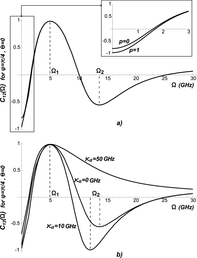
Figure 5: Cross-correlation spectrum $C_{12}(\Omega)$ for $\varphi=\pi/4$ and $\theta=0$; a) without dichroism, $\kappa_{a}=0$ and b) with dichroism, $\kappa_{a}=10\;GHz$ and $\kappa_{a}=50\;GHz$. The inset in a) illustrates the role of the statistical parameter $p$ at low spectral frequencies. All other parameters are as in Fig. 4.

In Fig. 5 we have plotted the cross-correlation spectrum $C_{12}(\Omega)$ for $\varphi=\pi/4$ and $\theta=0$. In this case the general result for $C_{12}(\Omega)$ given by Eqs. (73)-(74) is simplified to,

$$C_{12}(\Omega)=\frac{4\kappa\Bigl{[}(\delta X_{x}^{2})_{\Omega}-(\delta X_{y}^{2})_{\Omega}\Bigr{]}}{1+4\kappa\Bigl{[}(\delta X_{x}^{2})_{\Omega}+(\delta X_{y}^{2})_{\Omega}\Bigr{]}}.$$ (75)

Fig. 5a shows this cross-correlation spectrum for the case without dichroism and the same values of physical parameters as in Fig. 4. As follows from Fig. 5a, the cross-correlations are absent at high frequencies $\Omega$ larger than $30\;GHz$. At lower frequencies of the order of $15\;GHz$ the curve of $C_{12}(\Omega)$ shows anticorrelations which turn to correlations at still lower frequencies of the order of $5\;GHz$. In the area of low frequencies $\Omega$ smaller then $1\;GHz$ one has again anticorrelations.

This oscillating behavior of the cross-correlation spectrum $C_{12}(\Omega)$ is in full agreement with behavior of the fluctuation spectra of the Stokes parameters $S_{1}$ and $S_{2}$ in Fig. 4a. Indeed, the cross-correlation function $C_{12}(\Omega)$ is proportional to the difference of the spectral densities of the quadrature components $(\delta X_{x}^{2})_{\Omega}-(\delta X_{y}^{2})_{\Omega}$ [or the corresponding Stokes parameters, $(\delta S_{1}^{2})_{\Omega}-(\delta S_{2}^{2})_{\Omega}$]. Therefore, for $(\delta X_{x}^{2})_{\Omega}>(\delta X_{y}^{2})_{\Omega}$ we have correlations between the two photocurrents, while in the opposite case - anticorrelations.

Fig. 5b illustrates the same cross-correlation spectrum in presence of dichroism for different values of parameter $\kappa_{a}$. As mentioned above, the essential role of dichroism is in the suppression of the relaxation oscillations. When $\kappa_{a}$ approaches the critical value $\kappa_{a}=10\;GHz$ of the instability border, the relaxation oscillations grow up and reinforce anticorrelations. Further increase of $\kappa_{a}$ results in suppression of the relaxation oscillations and respectively in transformation of anticorrelations into correlations for $\kappa_{a}$ larger than $50\;GHz$.

IV.3 Cross-correlations between the Stokes parameters $S_{2}$ and $S_{3}$

For the $x$-polarized stationary solution that we consider in this paper, the linearized field operator $\vec{\hat{E}}(t)$ from Eq. (34) can be approximately written as,

$$\vec{\hat{E}}(t)=e^{i\Delta t}\Bigl{[}\sqrt{2}Q+\delta\hat{X}_{x}(t)+i\delta\hat{Y}_{x}(t)\Bigr{]}\Bigl{[}\vec{e}_{x}+\frac{1}{\sqrt{2}Q}(\delta\hat{X}_{y}(t)+i\delta\hat{Y}_{y}(t))\vec{e}_{y}\Bigr{]}.$$ (76)

This representation of the linearized field operator is very useful as it clarifies the physical meaning of the quantum fluctuations of the four quadrature components that appear in Eq. (76). The fluctuations $\delta\hat{X}_{x}(t)$ and $\delta\hat{Y}_{x}(t)$ describe respectively the quantum fluctuations of the amplitude and the phase of the electromagnetic field $\vec{\hat{E}}(t)$. The quantum fluctuations of two other quadrature components $\delta\hat{X}_{y}(t)$ and $\delta\hat{Y}_{y}(t)$ characterize the quantum fluctuations of the polarization of the field $\vec{\hat{E}}(t)$. To see this more clear let us compare Eq. (76) with the classical expression often used in the literature on VCSELs (see for example Ref. vanExter ),

$$\vec{\hat{E}}(t)\approx e^{i\Delta t}|E|\Bigl{[}\vec{e}_{x}-(\delta\phi+i\delta\chi)\vec{e}_{y}\Bigr{]}.$$ (77)

In this expression we have neglected the amplitude and the phase fluctuations of the field and have introduced the fluctuations $\delta\phi$ and $\delta\chi$, $\delta\phi\ll 1,\delta\chi\ll 1$ of two angles $\phi$ and $\chi$, that characterize the optical polarization state on the Poincaré sphere. The first angle $\phi\quad(0\leq\phi\leq\pi)$ is called the polarization angle and it determines the direction of the polarization ellipse. The second angle $\chi\quad(-\pi/4\leq\chi\leq\pi/4)$ is the ellipticity angle. For $x$-polarized field both of these angles are zero. Comparing Eq. (76) and Eq. (77) we conclude that these two classical fluctuations can be associated with their quantum counterparts as $\displaystyle{\delta\phi\rightarrow-\frac{\delta\hat{X}_{y}}{\sqrt{2}Q}}$ and $\displaystyle{\delta\chi\rightarrow-\frac{\delta\hat{Y}_{y}}{\sqrt{2}Q}}$. Taking into account Eq. (57) we can also write $\displaystyle{\delta\phi\rightarrow-\frac{\delta\hat{S}_{2}}{4Q^{2}}}$ and $\displaystyle{\delta\chi\rightarrow-\frac{\delta\hat{S}_{3}}{4Q^{2}}}$.

Thus, the quantum fluctuations of the Stokes parameter $S_{2}$ characterize the fluctuations of the polarization angle, and those of the $S_{3}$ - the fluctuations of the ellipticity angle. In the subsection A we have evaluated the fluctuation spectra of the Stokes parameters $S_{2}$ and $S_{3}$. However, as follows from Eq. (58) these two parameters are also cross-correlated. Hence, we shall introduce the cross-correlation spectrum $C_{23}(\Omega)$ between these two parameters in the same way as we did for characterization of the cross-correlations of two photocurrents,

$$C_{23}(\Omega)=\frac{(\delta S_{2}\delta S_{3})_{\Omega}}{\sqrt{(\delta S_{2}^{2})_{\Omega}}\sqrt{(\delta S_{3}^{2})_{\Omega}}}.$$ (78)

This cross-correlation spectrum is normalized as $|C_{23}(\Omega)|\leq 1$ and can be experimentally determined from the measurements of the following three photocurrent fluctuation spectra,

$$(\delta i^{2}_{-})_{\Omega}(45^{\circ},0^{\circ})/\langle i_{+}\rangle = 1+\frac{2\kappa}{Q^{2}}(\delta S_{2}^{2})_{\Omega},$$ (79)

$$(\delta i^{2}_{-})_{\Omega}(45^{\circ},90^{\circ})/\langle i_{+}\rangle = 1+\frac{2\kappa}{Q^{2}}(\delta S_{3}^{2})_{\Omega},$$ (80)

$$(\delta i^{2}_{-})_{\Omega}(45^{\circ},45^{\circ})/\langle i_{+}\rangle = 1+\frac{\kappa}{Q^{2}}\Bigl{[}(\delta S_{2}^{2})_{\Omega}+(\delta S_{3}^{2})_{\Omega}+2(\delta S_{2}\delta S_{3})_{\Omega}\Bigr{]}.$$ (81)

We have numerically evaluated the cross-correlation spectrum $C_{23}(\Omega)$ for the same values of physical parameters as in the previous subsection. In Fig. 6 we illustrate these spectra in the absence of dichroism $(\kappa_{a}=0)$ and for two different values of $\kappa_{a}$ equal to $10\;GHz$ and $50\;GHz$.

As follows from this figure, in the absence of dichroism the cross-correlation spectrum shows negative correlations at low frequencies $\Omega$ less than $10\;GHz$. These anticorrelations appear due to the coupling between the Stokes parameters $S_{2}$ and $S_{3}$ via the population difference $d$. For higher frequencies this coupling becomes less efficient and for $\Omega$ higher than $30\;GHz$ the fluctuations of $S_{2}$ and $S_{3}$ become independent $(C_{23}\rightarrow 0)$.

For nonzero dichroism the anticorrelations between $S_{2}$ and $S_{3}$ at low frequencies firstly disappear and then turn into positive correlations for larger values of $\kappa_{a}$, for example at $\kappa_{a}=50\;GHz$. Thus, dichroism changes the nature of correlations between $S_{2}$ and $S_{3}$.

V Conclusions

In conclusion we have presented a generalized and fully analytical theory of quantum fluctuations in VCSELs, proposed for the first time in Ref. Hermier02 . The original results of our investigation are the analytical expressions for the spectral densities of the quadrature field components and of the corresponding quantum Stokes parameters. These analytical results facilitate the comparison between the theory and the experimental measurements. Moreover, we have included into the theory a nonzero linear dichroism of the semiconductor medium that was neglected in Ref. Hermier02 .

Our theory is very closely related to possible experimental observation of the quantum fluctuations in VCSEls that can be performed in a correlation-type measurement shown in Fig. 3. We have calculated analytically and illustrated graphically the typical fluctuation and cross-correlation spectra that could be observed in this type of measurements. Our theoretical results allow for direct comparison with experiments.

We predict theoretically polarization squeezing in VCSELs when the quantum fluctuations of the Stokes parameter $S_{1}$ are reduced below the standard quantum limit. This phenomenon has its origin in regular pumping statistics of the active laser medium. However, the regularity in the pumping statistics alone is not sufficient for polarization squeezing in this type of lasers due to the partition noise between two upper sublevels in the laser medium. The second important feature of VCSELs that guarantees polarization squeezing is their dynamical behavior that couples the statistical properties of the Stokes parameter $S_{1}$ only with those of the total population of two upper sublevels.

We have analyzed the role of linear dichroism and have concluded that it mainly influences the relaxation oscillations in VCSEls. These oscillations are typical for the solid-state and semiconductor lasers. The particularity of VCSEls is that in this case there are two types of relaxation oscillations with clearly distinct characteristic frequencies $\Omega_{1}$ and $\Omega_{2}$. First oscillations (with frequency $\Omega_{1}$) are related to the total population of two upper sub-levels and they contribute to the fluctuation spectrum of the Stokes parameter $S_{1}$. The second type of relaxation oscillations (with frequency $\Omega_{2}$) is connected with the population difference and its peak appears in the fluctuation spectra of the Stokes parameters $S_{2}$ and $S_{3}$. It turns out the dichroism dumps the relaxation oscillations of the second type and does not influence those of the first type. To understand this result let us recall that the relaxation oscillations appear in the lasers of the second type when the resonator losses are more rapid compared with those of the laser medium. As follows from Eqs. (17) and (18) dichroism increases the losses for the $y$-polarized light component coupled with the population difference $d$ and does not change those of the $x$-polarized component related to population sum $D$.

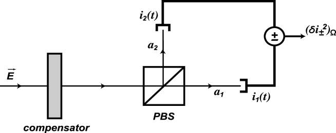
Figure 3: Experimental scheme for measurement of the spectral densities and cross-spectral densities of the quantum Stokes parameters.

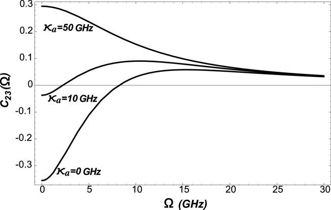
Figure 6: Cross-correlation spectrum $C_{23}(\Omega)$ without dichroism, $\kappa_{a}=0$ and with dichroism, $\kappa_{a}=10\;GHz$ and $\kappa_{a}=50\;GHz$ for the same values of physical parameters as in Fig. 4.

- (1) J.-P. Hermier, M. I. Kolobov, I. Maurin, and E. Giacobino, Phys. Rev. A 65, 053825 (2002).
- (2) P. Schnitzer, M. Grabherr, R. Jager, F. Mederer, R. Michalzik, D. Wiedenmann, and K. J. Ebeling, IEEE Phot. Tech. Lett. 11, 769 (1999).
- (3) Y. M. Golubev and I. V. Sokolov, Sov. Phys. JETP 60, 234 (1984).
- (4) Y. Yamamoto, S. Machida, and O. Nilsson, Phys. Rev. A 34, 4025 (1986).
- (5) C. Degen, J. L. Vey, W. Elsäßer, P. Schnitzer, and K. J. Ebeling, Elect. Lett. 34, 1585 (1998).
- (6) J. P. Hermier, A. Bramati, A. Z. Khoury, V. Josse, E. Giacobino, P. Schnitzer, R. Michalzik, and K. J. Ebeling, IEEE J. Quant. Elect. 37, 87 (2001).
- (7) M. P. van Exter, M. B. Willemsen, and J. P. Woerdman, Phys. Rev. A 58, 4191 (1998).
- (8) M. B. Willemsen, M. P. van Exter, and J. P. Woerdman, Phys. Rev. A 60, 4105 (1999).
- (9) M. San Miguel, Q. Feng, and J. V. Moloney, Phys. Rev. A, 52, 1728 (1995).
- (10) M. P. van Exter, A. Al-Remawi, and J. P. Woerdman, Phys. Rev. Lett. 80, 4875 (1998).
- (11) M. P. van Exter, M. B. Willemsen, and J. P. Woerdman, J. Opt. B: Quantum Semiclass. Opt. 1, 637, (1999).
- (12) J. Mulet, C. R. Mirasso, and M. San Miguel, Phys. Rev. A 64, 023817 (2001).
- (13) W. W. Chow, S. W. Koch, and M. Sargent III, Semiconductor-Laser Physics (Springer-Verlag, Berlin, 1994).
- (14) C. Benkert, M. O. Scully, J. Bergou, L. Davidovich, M. Hillery, and M. Orszag, Phys. Rev. A 41, 2756 (1990).
- (15) M. I. Kolobov, L. Davidovich, E. Giacobino, and C. Fabre, Phys. Rev. A 47, 1431 (1993).
- (16) J. Martin-Regalado, F. Prati, M. San Miguel, and N. B. Abraham, IEEE J. Quantum Electron. 33, 765 (1997).
- (17) Yu. M. Golubev, T. Yu. Zernova, and E. Giacobino, Opt. Spectrosc. 94, 75 (2003).
- (18) M. Born and E. Wolf, Principles of Optics, 7th ed. (Cambridge University Press, Cambridge, England, 1999).
- (19) J. M. Jauch and F. Rohrlich, The Theory of Photons and Electrons (Springer, Berlin, 1976).
- (20) B. A. Robson, The Theory of Polarization Phenomena (Clarendon Press, Oxford, 1974).
- (21) A. S. Chirkin, A. A. Orlov, and D. Yu. Paraschuk, Quantum Electron. 23, 870 (1993).
- (22) D. N. Klyshko, JEPT 84, 1065 (1997).
- (23) N. V. Korolkova and A. S. Chirkin, Quantum Electron. 24, 805 (1994).
- (24) A. S. Chirkin and V. V. Volokhovsky, J. Russ. Laser Res. 16, 6 (1995).
- (25) A. P. Alodjants, A. M. Arakelian, and A. S. Chirkin, JETP 108, 63 (1995).
- (26) N. V. Korolkova and A. S. Chirkin, J. Mod. Opt. 43, 869 (1996).
- (27) N. Korolkova, G. Leuchs, R. Loudon, T. C. Ralph, and C. Silberhorn, Phys. Rev. A 65, 052306 (2002).
- (28) P. Grangier, R. E. Slusher, B. Yurke, and A. LaPorta, Phys. Rev. Lett. 59, 2153 (1987).
- (29) V. P. Karasev and A. V. Masalov, Opt. Spectrosc. 74, 551 (1993).
- (30) P. A. Buchev, V. P. Karassiov, A. V. Masalov, and A. A. Putilin, Opt. Spectrosc. 91, 526 (2001).
- (31) W. P. Bowen, R. Schnabel, H.-A. Bachor, and P. K. Lam, Phys. Rev. Lett. 88, 093601 (2002).