Ergodic quantum computing

Abstract

We propose a (theoretical  ;-) model for quantum computation where the result can be read out from the time average of the Hamiltonian dynamics of a $2$-dimensional crystal on a cylinder. The Hamiltonian is a spatially local interaction among Wigner-Seitz cells containing $6$ qubits. The quantum circuit that is simulated is specified by the initialization of program qubits. As in Margolus’ Hamiltonian cellular automaton (implementing classical circuits), a propagating wave in a clock register controls asynchronously the application of the gates. However, in our approach all required initializations are basis states. After a while the synchronizing wave is essentially spread around the whole crystal. The circuit is designed such that the result is available with probability about $1/4$ despite of the completely undefined computation step. This model reduces quantum computing to preparing basis states for some qubits, waiting, and measuring in the computational basis. Even though it may be unlikely to find our specific Hamiltonian in real solids, it is possible that also more natural interactions allow ergodic quantum computing.

1 Introduction

The question which control operations are necessary to achieve universal quantum computing is essential for quantum computing research. The standard model of quantum computation requires (1) preparation of basis states, (2) implementation of single and two-qubit gates and (3) single-qubit measurements in the computational basis. Meanwhile there are many proposals that reduce or modify the set of necessary control operations (see e.g. [1, 2, 3, 4, 5]). Common to all those models is that the program is encoded in a sequence of control operations.

Here we consider a model which requires no control operations during the computation since the computation is carried out by the autonomous time evolution of a fixed Hamiltonian. The idea to consider theoretical models of computers which consist of a single Hamiltonian can already be found in [6, 7, 8]. However, these models are not explicitly designed for implementing quantum algorithms. We start from Margolus’ approach since it has the attractive property that the Hamiltonian is a homogeneous spatially local interaction between cells of a $2$-dimensional lattice and is therefore “relatively close” to interactions in crystals. Margolus’ Hamiltonian implements the dynamics of a classically universal cellular automaton (CA). In his two-dimensional model the front of a spin wave propagates in one direction over the surface and controls the updating of the cells. Even though there is no globally controlled clocking of the updates his local synchronization ensures that each cell is not updated until all relevant neighbors are already updated. In the Margolus scheme the computer is always in a superposition of many computation steps. At the beginning one has to prepare the wave front such that it mainly propagates in the forward direction. Such a state is not a computational basis state. We found it intriguing to use only basis states. Our goal was to reduce the required control operations to the absolute minimum: input of the initial state, the writing of the program and the readout of the classical output. The basis states we start with consist of components propagating forward and components propagating backward. Our circuit is designed such that even the backward computation leads to the correct result. When the time average of an appropriate initial state subjected to the Hamiltonian dynamics is measured one obtains the correct result with high probability. The state tells us whether the result has to be rejected. Hence one may consider the procedure as a Las Vegas algorithm. Our Hamiltonian is a sum of operators which act on $10$ qubits in contrast to the $2$-dimensional Margolus cellular automaton which needs interactions between $8$ qubits for universal classical computation. In [9] one finds a $4$-local Hamiltonian where the time average of a single qubit encodes the answer of a PSPACE hard problem. But the Hamiltonian has to be constructed for the specific PSPACE problem. The Hamiltonian is not homogeneous and is not appropriate for universal computation.

The structure of the paper is as follows. In Section 2 we choose a set of four $2$-qubit gates which is universal for quantum computing. In Section 3 we construct a $4$-qubit gate which includes all these $4$ gates into one controlled gate. This makes the computer programmable. Then we describe how the synchronization scheme of Margolus is used: A wave front of a clock register propagating around the cylinder ensures that the programmable gates are applied in correct time order. This propagation is done by the evolution of an appropriate Hamiltonian. In Section 4 we describe the symmetry of the crystal by the crystallographic concept of Wigner-Seitz cells. In Section 5 we prove that the time average leads to the correct result. The readout of this result is explicitly described in Section 6. In Section 7 we briefly show that ergodic quantum computing can in principle solve all problems in polynomial space for all problems where usual quantum algorithms need only polynomial space. At first sight, this seems to be in contradiction to the fact that time steps of usual algorithms are translated to spatial propagation (as in [1]).

2 Universal set of gates

We recall [10] that the following types of gates are sufficient for universal quantum computation. Let $({\mathbb{C}}^{2})^{\otimes n}$ be the state space of a quantum register. Then we consider the following two-qubit and single-qubit gates which are assumed to be available for every pair of qubits or every single qubit, respectively:

1. The Hadamard gate on a single qubit:

   $$H:=\frac{1}{\sqrt{2}}\left(\begin{array}[]{cc}1&1\\ 1&-1\end{array}\right)$$

2. The controlled-phase gate

   $$\Gamma(\sigma^{1/2}_{z})=|1\rangle\langle 1|\otimes\frac{1}{\sqrt{2}}\left(\begin{array}[]{cc}1&0\\ 0&i\end{array}\right)+|0\rangle\langle 0|\otimes{\mathbf{1}}$$

   where $|0\rangle,|1\rangle$ are the canonical basis states of ${\mathbb{C}}^{2}$ and ${\mathbf{1}}$ is the identity.

Note that an exact implementation of the SWAP gate is possible. Therefore, without losing universality, we allow the application of controlled phase gates only on adjacent qubits.

We assume that gates acting on disjoint sets qubits can be applied at the same time step. We call such a time step a layer of the quantum circuit. The depth of the quantum circuit is the number of time steps.

For reasons that shall be clear later we consider circuits $U$ which have a special layer structure (see Fig. 1). Each time step consists of several gates with the following restrictions:

• In even time-steps we allow only two-qubit gates acting on the qubit pairs $(k,k+1)$ with even $k$.

• In odd time-steps we have only two-qubits gates on $(k,k+1)$ with odd $k$.

In this scheme we distinguish formally among four $2$-qubit gates:

$$U_{00}:={\mathbf{1}}\otimes{\mathbf{1}}\,,\quad U_{01}:={\mathbf{1}}\otimes H\,,\quad U_{10}:=H\otimes{\mathbf{1}}\,,\quad U_{11}:=\Lambda(\sigma_{z}^{1/2})\,.$$ (1)

Figure 1: Decomposition of arbitrary quantum circuits into layers of two-qubit gates $U_{00},\ldots,U_{11}$ acting on adjacent pairs.

Using these gates, we construct a circuit $U$ with the following properties: Let $f:\{0,1\}^{n}\rightarrow\{0,1\}^{m}$ be the function we would like to compute. The unitary $U$ acts on the input, the output register, and some ancilla register and computes $f$ in the sense

$$U\big{(}|x\rangle\otimes|y\rangle\otimes|0\dots 0\rangle\big{)}=|x\rangle\otimes|y\oplus f(x)\rangle\otimes|0\dots 0\rangle\,,$$

where $\oplus$ denotes the bitwise XOR. By construction, we have

$$U^{2}\big{(}|x\rangle\otimes|y\rangle\otimes|0\dots 0\rangle\big{)}=|x\rangle\otimes|y\rangle\otimes|0\dots 0\rangle\,.$$

Without loss of generality, we may assume that $f(x)\neq 0$ for all inputs $x$ by extending $f$ with an additional bit which is always $1$.

Note that there are quantum algorithms where $f(x)$ is only computed probabilistically. We will neglect this fact since it is irrelevant for the principles of our construction and would make the discussion unnecessarily technical.

3 Constructing the crystal Hamiltonian

Usually a quantum circuit is considered as a sequence of gates. However, the usual way of drawing it (like in Fig. 1) suggests spatial propagation. Now we consider quantum circuits where quantum information is really spatially propagated and the time-axis is represented by the second dimension.

Our circuit is wrapped around a cylinder. The cylinder is covered by $c\times h$ squares (“cells”) of equal size. We have $h$ (for “height”) columns and $c$ (for “circumference”) rows. We need $c>2h$ for reasons which will be clear in Section 6. The columns correspond to the qubits of the original circuit and the rows to its time steps (see fig.2).

         

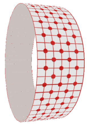
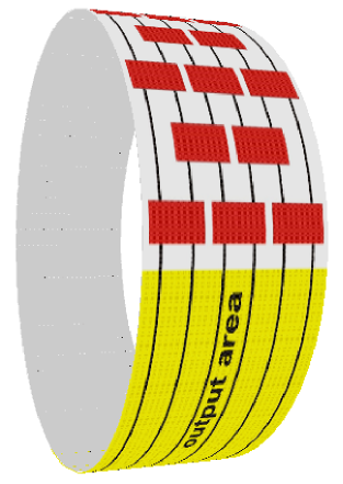
Figure 2: (Left) Cylindric crystal consisting of $c\times h$ cells. A pair of program qubits is located at the red points. The lines indicate the boundaries of a cell. (Right) The circuit wrapped around the cylinder. Every time when a two-qubit gate is applied the information of both qubits is propagated one row upwards. The output region consists only of trivial gates, i.e. the information is only propagated.

Each cell $(j,k)$ contains a data qubit. They form the data space

$${\cal H}_{D}:=({\mathbb{C}}^{2})^{\otimes ch}\,.$$

In the $j$-th time step we apply all gates of layer $j$. A gate of the original circuit acting on the qubit pair $(k,k+1)$ in level $j$ translates to a gates acting on data qubits in cells $(j,k),(j,k+1),(j+1,k),(j+1,k+1)$. It applies the original two-qubit gate to the qubits in row $j$ and propagates the information to row $j+1$. Furthermore, the vertices between those $4$ cells contain two program qubits which specify which one of the two-qubit gates in eq. (1) should be applied. Explicitly, there are two qubits between cell $(j,k)$ and $(j+1,k+1)$ if both $k$ and $j$ are even or both are odd (see Fig. 2). For each vertex with program qubits we define the gate

$$V:=W\sum_{l,m\in\{0,1\}\times\{0,1\}}P_{lm}\otimes U_{lm}\,.$$ (2)

where $P_{jm}:=|jm\rangle\langle lm|$ projects onto the state $|lm\rangle$ of the two-qubit program register at a certain vertex. $W$ is the swap gate which exchanges the state of the qubit pairs $(j,k)$ and $(j+1,k)$ and the pairs $(j,k+1)$ and $(j+1,k+1)$.

This makes our system programmable and will be essential for achieving our goal to construct a universal Hamiltonian which can simulate all circuits. We will only write a program on some part of the cylinder because we need the other part as output region (see Section 6). As we have already stated, a computation would consist of applying all gates in row $j$ in the $j$-th step. However, this requirement is unnecessarily strong. Actually, the only rule is that each gate in row $j$ can only be applied if both gates in row $j-1$ which contribute to its input have been applied. These synchronization rules can be visualized by building walls with bricks (see fig. 3). The synchronization conditions mean intuitively that incorrect walls are not allowed. In order to make this analogy perfect we introduce dummy single qubit gates at the boundaries of odd rows.

                 

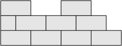
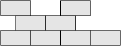
Figure 3: Correct (left) and incorrect (right) walls. Putting a brick at position $k,j$ corresponds to carrying out the gate in level $j$ acting on the qubit pair $(j,k)$ and $(j,k+1)$.

We would like to construct a Hamiltonian such that its autonomous time-evolution corresponds to a computation which respects these synchronization rules. Margolus [11] solved this problem by introducing clock qubits as follows.

Each cell contains a clock qubit. Let ${\cal H}_{C}=({\mathbb{C}}^{2})^{\otimes ch}$ be the Hilbert space of all these clock qubits. Define the operator

$$G_{j,k}:=\begin{array}[]{ccc}a^{\dagger}&\otimes&a^{\dagger}\\ \otimes&&\otimes\\ a&\otimes&a\end{array}\,,$$

where the annihilation operators $a$ act on the qubits $(j,k)$ and $(j,k+1)$ and the creation operators $a^{\dagger}$ act on the qubits $(j+1,k)$ and $(j+1,k+1)$. These operator $G_{j,k}$ propagate two $1$’s in the qubits $(j,k)$ and $(j,k+1)$ one row upwards

$$\begin{array}[]{|cc|}\hline\cr 0&0\\ 1&1\\ \hline\cr\end{array}\quad\mapsto\quad\begin{array}[]{|cc|}\hline\cr 1&1\\ 0&0\\ \hline\cr\end{array}\,,$$

where the left lower corner of the cell is at position $(j,k)$. All other configurations are mapped onto the zero vector. Now we define the operator

$$G:=\sum_{j,k}G_{j,k}$$

where $j=0,\ldots,c-1$ and

$$k=\left\{\begin{array}[]{ll}0,2,\ldots,h-2&\mbox{ for $j$ even}\\ 1,3,\ldots,h-3&\mbox{ for $j$ odd}\end{array}\right.\,.$$ (5)

In contrast to Margolus we do not consider a cyclic system in both axis but only cyclic in one direction. This is because we think that a crystal with $2$-dimensional torus symmetry seems less realistic.

At the boundary we define a family of operators which act on only two adjacent cells: For each odd $j$ we set

$$G_{j,-1}:=\frac{1}{\sqrt{2}}\,\begin{array}[]{c}a^{\dagger}\\ \otimes\\ a\end{array}\,,\quad\quad G_{j,h-1}:=\frac{1}{\sqrt{2}}\,\begin{array}[]{c}a^{\dagger}\\ \otimes\\ a\end{array}\,,$$ (6)

where the annihilation operators act on the qubits $(j,0)$ and $(j,h-1)$ and the creation operators act on the qubits $(j+1,0)$ and $(j+1,h-1)$, respectively. These operators propagate a $1$ in the qubits $(j,0)$ and $(j,h-1)$, respectively, one row upwards

$$\begin{array}[]{|c|}\hline\cr 0\\ 1\\ \hline\cr\end{array}\quad\mapsto\quad\begin{array}[]{|c|}\hline\cr 1\\ 0\\ \hline\cr\end{array}\,,$$

where the left lower corner of the rectangle is at position $(j,k)$ with $j$ odd and $k=0,h-1$. All other configurations are mapped onto the zero vector. Now we include these operators in the operator $G$.

Now we define a $G$-invariant subspace ${\cal H}_{C}$, interpreted as the space of correct synchronizations. Intuitively, it is spanned by the set of all basis states corresponding to correct walls. The position of the uppermost brick in each column is denoted by symbols $1$ as in fig. 4.

Figure 4: Visualization of the basis states of $\tilde{{\cal H}}_{C}$ (the space of allowed clock states) as brick walls.

Lemma 1 (Synchronization space)

Let $\tilde{{\cal H}}_{C}$ be the space spanned by those basis vectors $|a\rangle$, where $a$ is a $0$-$1$-matrix of size $c\times h$ satisfying the following conditions:

1. Each column contains a single $1$, the remaining entries are all $0$.

2. Let $j_{k}$ be the index of the symbol $1$ in column $k$. Then for the indices of any two adjacent columns $k$ and $k+1$ we have

   $$|j_{k}-j_{k+1}|\leq 1\,.$$

3. If $k+j_{k}$ is even then

   $$j_{k}\geq j_{k+1}\,.$$

   If $k+j_{k}$ is odd then

   $$j_{k}\leq j_{k+1}\,.$$

Then $\tilde{{\cal H}}_{C}$ is $G$-invariant.

Proof. Let $a$ be any configuration satisfying the above conditions.

• Applying $G_{j,k}$ to $|a\rangle$ does not lead to the zero vector iff the symbol $1$ is at position $j$ in the adjacent columns $k$ and $k+1$, i. e., $j_{k}=j_{k+1}=j$. If this is the case, then $G_{k,j}$ propagates both $1$’s one position upward. Therefore, the configuration $G_{k,j}|a\rangle$ still fulfills condition (1).

• Assume first that $a$ is a configuration with $j_{k}>j_{k+1}$ for some $k$. Since $a$ satisfies condition (2) we know that $j_{k}=j_{k+1}+1$. The only operators which act on qubit $(k,j_{k})$ are $G_{j_{k},k}$ and $G_{j_{k}-1,k-1}$. The $G_{j_{k},k}$ operator vanishes when applied to $|a\rangle$ because the symbol $1$ is at position $j_{k}-1$ in column $k+1$ and not at position $j_{k}$ which would be required for a non-trivial action of $G_{j,k}$. The operator $G_{j_{k}-1,k-1}$ vanishes because the $1$ is at position $j_{k}$ in column $k$ and not at position $j_{k}-1$ as would be required for a non-trivial action of $G_{j_{k}-1,k-1}$. This situation is shown on the left in fig. 5.

                            

  Figure 5: Left: the application of the operators corresponding to the squares annihilate the state. Right: The application of the operator which corresponds to the upper square propagates both symbols $1$.

  The case $j_{k}<j_{k+1}$ is proved analogously.

• Assume that $a$ is a configuration with $j_{k}=j_{k+1}$ for some pair of adjacent columns $k$ and $k+1$. Let $k+j_{k}$ be even. In this case we have to show that every action which increases $j_{k+1}$ also increases $j_{k}$.

  We first consider the case that both $k$ and $j_{k}$ are even. The only operators that act on the qubit $(k+1,j_{k+1})=(k+1,j_{k})$ are $G_{k,j_{k}}$ and $G_{k+1,j_{k}-1}$. The second operator vanishes because the symbol $1$ is not at position position $j_{k}-1$ in the column $k+1$ but at $j_{k}$. The operator $G_{k,j_{k}}$ increases $j_{k}$ and $j_{k+1}$ as claimed. This situation is shown on the right in fig. 5.

  Analogously, we can prove that this is also true if $k$ and $j_{k}$ are both odd. The remaining case is that $k+j_{k}$ is odd. By using analogous arguments we can show that every action which increases $j_{k}$ also increases $j_{k+1}$.

$\Box$

In analogy to Margolus’ and Feynman’s ideas we define the forward time operator $F$ by

$$F:=\sum_{j,k}G_{j,k}\otimes V_{j,k}$$

where $V_{j,k}$ is the gate $V$ in eq. (2) acting on the qubits $(j,k)$,$(j,k+1)$,$(j+1,k)$, and $(j+1,k+1)$. For the operators $G_{j,-1}$ and $G_{j,h-1}$ ($j$ odd) at the boundary we set $V_{j,-1}:={\mathbf{1}}$ and $V_{j,h-1}:={\mathbf{1}}$.

The Hamiltonian is defined as the sum of the forward time operator and backward time operator

$$H:=F+F^{\dagger}\,.$$

In the sense of [12] this is a $10$-local interaction since each operator $G_{j,k}$ acts on $10$ qubits at once. Note that one may rewrite the interactions as $k$-local terms with $k<10$ by introducing qudits, i.e., particles with higher dimensional Hilbert spaces. Therefore the size $10$ does not necessarily mean that this interaction is unphysical.

To analyze the dynamical evolution we need the feature that $F$ is a normal operator on the relevant subspace (analog to Margolus’ results). However, since we do not work with cyclic boundary conditions the proof is a little bit more technical. As noted in [13] the dynamics of the $1$-dimensional cyclic Margolus Hamiltonian [11] is the quasi-free time evolution of independent fermions.

Even though we do not see if the clock dynamics of our Hamiltonian is also quasi-free, we can prove:

Lemma 2

The restriction of $F$ to the relevant space

$${\cal H}:=\tilde{{\cal H}}_{C}\otimes{\cal H}_{D}\otimes{\cal H}_{P}$$

is normal, i.e., $FF^{\dagger}=F^{\dagger}F$.

Proof. For an initial state $|\psi\rangle\in{\cal H}$ the operator $FF^{\dagger}|\psi\rangle$ is a sum of terms of the form

$$F_{j,k}F^{\dagger}_{\tilde{j},\tilde{k}}|\psi\rangle\,.$$ (7)

$F^{\dagger}F|\psi\rangle$ is a sum of terms of the form

$$F^{\dagger}_{\tilde{j},\tilde{k}}F_{j,k}|\psi\rangle\,.$$ (8)

For $|k-\tilde{k}|\geq 2$ or $|j-\tilde{j}|\geq 2$ the operators $F^{\dagger}_{\tilde{j},\tilde{k}}$ and $F_{j,k}$ act on disjoint qubits and thus commute. Then the products in eq. (7) and eq. (8) are equal.

If $|k-\tilde{k}|\leq 1$ and $|j-\tilde{j}|\leq 1$ then it is easily checked that the product $G^{\dagger}_{\tilde{j},\tilde{k}}G_{j,k}|a\rangle$ is only non-zero for $(j,k)=(\tilde{j},\tilde{k})$.

Therefore, it is sufficient to show that

$$\sum_{(j,k)}F_{j,k}F^{\dagger}_{j,k}|\psi\rangle=\sum_{(j,k)}F^{\dagger}_{j,k}F_{j,k}|\psi\rangle$$ (9)

in order to prove that $F$ is normal. Since the operators $U_{j,k}$ are unitary it is sufficient to show that

$$\sum_{(j,k)}G_{j,k}G^{\dagger}_{j,k}|a\rangle=\sum_{(j,k)}G^{\dagger}_{j,k}G_{j,k}|a\rangle$$ (10)

for every allowed clock configuration $a$. Note that $|a\rangle$ is an eigenvector of the operators on both sides since each term which does not vanish is identical to a multiple of the vector $|a\rangle$. First we consider only the operators $G_{j,k}$ which act on $4$ clock qubits and not the special operators $G_{j,-1}$ and $G_{j,h-1}$ at the boundaries. In the cyclic model of Margolus, the right-hand term in (10) counts the possibilities to go forward and the left-hand term the possibilities to go backward. The fact that both numbers coincide prove normality. in the non-cyclic case the possibilities to add or remove half bricks have to be considered separately.

Note that $G_{j,k}|a\rangle$ can only be non-zero if $j=j_{k}$ (with $j_{k}$ defined as in Lemma 1), i.e., there is the symbol $1$ in position $j$ in the $k$th column. Then the term $G_{j_{k},k}|a\rangle$ does not vanish if and only if there is also a symbol $1$ in position $(j_{k},k+1)$.

To formalize these conditions we introduce the variable $c_{k}:=(j_{k}+k)\pmod{2}$ indicating whether $j_{k}+k$ is even or odd. Due to the definition of the operators $G_{j,k}$ the term $G_{j_{k},k}|a\rangle$ is only non-zero if $c_{k}=0$. The position of the second symbol $1$ requires $c_{k+1}=1$. Since $j_{k+1}$ can differ from $j_{k}$ by at most $1$ the conditions

$$c_{k}=0\hbox{ and }c_{k+1}=1$$

are also sufficient that $G_{j_{k},k}|a\rangle$ is non-zero.

Similarly, we have $G_{j_{k},k}G^{\dagger}_{j_{k},k}|a\rangle=|a\rangle$ whenever

$$c_{k}=1\hbox{ and }c_{k+1}=0\,.$$

Let $n_{10}$ and $n_{01}$ be the number of occurrences of the patterns $10$ and $01$ in the string $(c_{0},\ldots,c_{h-1})$, respectively. If $n_{10}=n_{01}$ then the leftmost and the rightmost symbols coincide. In both cases exactly one of the boundary terms

$$G^{\dagger}_{j_{0},-1}G_{j_{0},-1}|a\rangle\,,\quad G^{\dagger}_{j_{h-1},h-1}G_{j_{h-1},h-1}|a\rangle$$

does not vanish and yields the vector $(1/2)|a\rangle$. The same is true for the terms with the conjugated boundary operators. Hence both sides of eq. (10) yield the same vector $(n+1/2)|a\rangle$.

Note that $n_{10}$ and $n_{01}$ can differ by at most one. This is the case if and only if the leftmost and the rightmost symbol are different. If $n_{10}=n_{01}+1$ the leftmost and the rightmost symbols are $1$ and $0$, respectively. If $n_{01}=n_{10}+1$ they are $0$ and $1$, respectively. In the first case only the combinations

$$G^{\dagger}_{j_{0},-1}G_{j_{0},-1}|a\rangle\,,\quad G^{\dagger}_{j_{h-1},h-1}G_{j_{h-1},h-1}|a\rangle$$

lead to non-zero terms and contribute to the right-hand side of eq. (10) with $(1/2)|a\rangle$ each. The conjugated boundary operators lead both to vanishing terms. This fact compensates the difference of $1=n_{10}-n_{01}$ in the contribution to the left-hand and the right-hand side of eq. (10). The second case ($n_{01}=n_{10}+1$) is treated analogously. $\Box$

The fact that $F$ is normal helps to understand the dynamical evolution according to $F+F^{\dagger}$. In [11] this fact makes it possible to find a conserved quantity interpreted as the computation speed. It is given by the operator $V:=(F-F^{\dagger})/i$. Then Feynman and Margolus start with initial states which have a positive expectation value of the computation speed. Their initial states are necessarily superpositions of basis states because the expectation value of $V$ is zero for every basis state of the clock. Since $|\psi\rangle$ is orthogonal to $F|\psi\rangle$ and $F^{\dagger}|\psi\rangle$ we have $\langle\psi|F-F^{\dagger}|\psi\rangle=0$ with $|\psi\rangle:=|a\rangle\otimes|\phi\rangle$, where $|\phi\rangle\in{\cal H}_{P}\otimes{\cal H}_{D}$ and $a$ is an allowed clock configuration. In our approach, all initial states are basis states. Despite these differences, normality of $F$ will be essential in Section 5 for the “ergodic theory” of our Hamiltonian.

4 Symmetry of the crystal

The symmetry of a crystal can be described by a unit cell such that the whole lattice consists of shifted unit cells where the translations are integer multiples of the lattice vectors. A usual way to choose unit cells is given by the so-called Wigner-Seitz cell [14]. It is constructed as follows. Consider an arbitrary point $Q$ in the lattice and consider the set of all points $Q^{\prime}$ which are equivalent to $Q$ in the sense that the translation $QQ^{\prime}$ is a symmetry operation. Consider the perpendicular bisector of the side $QQ^{\prime}$. It divides ${\mathbb{R}}^{2}$ into two half-planes containing $Q$ and $Q^{\prime}$, respectively. Then the Wigner-Seitz cell (WS cell) is the intersection of all half planes containing $Q$. Here we choose the position of one pair of program qubits (i.e., a thick red point in fig. 2) as $Q$. In the sequel we will refer to our original cells simply as cells in contrast to the WS cell. A WS cell is a square which has double area compared to the original cells and is rotated by $45^{\circ}$. It covers $4$ adjacent cells such that it contains half of the area of each. This is depicted in fig. 6.

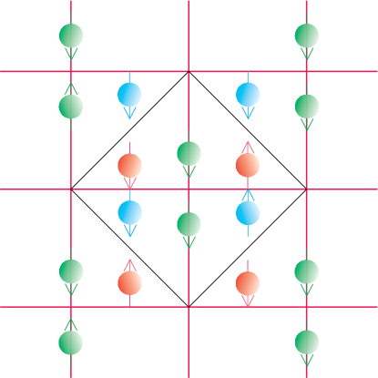
Figure 6: The black square is a Wigner-Seitz cell containing $6$ qubits. The program bits are green, the clock qubits are red and the data qubits blue. The red grid indicates the original cells.

We locate the data and clock spins of each cell such that the WS cell (which is centered around $2$ program qubits) contains $2$ clock qubits and $2$ data qubits. Hence, the WS cell contains $6$ qubits. Each WS cell interacts with those adjacent WS cell which have an edge in common. Note, however, that the interaction among the WS cells are not pair-interactions between adjacent WS cells because it contains operators which act on $5$ WS cells at once (note that the operators $F_{j,k}$ involve $4$ cells).

Note that the crystal is symmetric under reflections at columns. due to the symmetry of the controlled $\Lambda(\sigma_{z}^{1/2})$-gate. The crystal, as we defined it, is not symmetric under reflections at rows.

5 Mixing properties of the time evolution

Our crystal Hamiltonian $H=F+F^{\dagger}$ is (on the relevant subspace) two times the real part of the normal operator $F$. Therefore, $F$ and $H$ have a common spectral decomposition. The following property of $F$ is essential:

Let $|\psi\rangle:=|a\rangle\otimes|\phi\rangle\in{\cal H}$ be an initial state of clock, program, and data register, where $a\in\{0,1\}^{ch}$ is an allowed clock configuration. Let $g:=(h+1)c/2$ be the number of bricks (where half bricks are counted like full bricks) needed to cover the whole cylindric surface. Then we have

$$F^{j}|\psi\rangle\perp F^{k}|\psi\rangle$$ (11)

for all $j\neq k\mod g$. This is easily checked because each state $F^{j}|\psi\rangle$ is a superposition of states where “the wall” is enlarged by $j$ bricks. In order to get the same clock configuration one needs to add a multiple of $g$ bricks. Note that the quantum circuit $U$ (which is encoded in the program register) can be constructed in such a way that the orthogonality relation (11) holds even for all $j\neq k\mod 2g$. Consider, for instance, the case $j=k+g$. Project both states in (11) onto the subspace of ${\cal H}$ induced by a definite clock configuration $a$. On this subspace, the states of the data register differ by some unitary. This unitary $U^{\prime}$ is given by the concatenation of all those gates which have to be applied in order to go from the clock state $a$ to $a$ again by winding around the cylinder once. In other words, $U^{\prime}$ is obtained by splitting the circuit $U$ and reversing the order of both parts as follows: Let $U_{1}$ be given by the sequence of gates which are applied when the clock wave moves from its initial position to $a$. Analogously, $U_{2}$ is given by all gates that are applied when the clock wave moves from $a$ to the initial position. Then $U^{\prime}$ is given by $U^{\prime}:=U_{1}U_{2}$ and $U=U_{2}U_{1}$.

If at least one bit of the computed value $f(x)$ is $1$ the application of $U$ leads always to orthogonal states in the data register. Hence the orthogonality relation (11) is already satisfied for $j=g$ and $k=0$. This corresponds to the trivial splitting $U_{1}=U$ and $U_{2}={\mathbf{1}}$. Unfortunately, the bit flip which occurs on one of the output bits cannot be implemented by one gate since classical gates are not available in our setting. Therefore the other splittings may divide the flip operation into non-classical operations. In order to guarantee that also the other splittings lead to orthogonal data states we may construct $U$ in such way that it flips two bits, one at the beginning and one at the end. Then either $U_{1}$ or $U_{2}$ contain one complete bit flip.

The following lemma is important for analyzing the ergodic behavior since it shows that $F$ is essentially a copy of the shift operator acting on mutually orthogonal spaces:

Lemma 3

Let $B$ be a normal operator on a finite-dimensional Hilbert space ${\cal H}$ and $|\Psi\rangle\in{\cal H}$ such that

$$B^{j}|\psi\rangle\perp B^{k}|\psi\rangle\quad\quad j\neq k\mod N$$

for some $N\in{\mathbb{N}}$. Define

$${\cal H}_{l}:={\rm span}_{j\in{\mathbb{N}}_{0}}\{B^{l+jN}|\psi\rangle\}\,,$$

where $l=0,\ldots,N-1$ and $\hat{{\cal H}}:=\oplus_{l=0}^{N-1}{\cal H}_{l}$. Then only the following two cases can occur:

1. All ${\cal H}_{l}$ have the same dimension $r$. Then we may identify $\hat{{\cal H}}$ with ${\mathbb{C}}^{N}\otimes{\mathbb{C}}^{r}$ such that ${\cal H}_{l}$ corresponds to $|l\rangle\otimes{\mathbb{C}}^{r}$ and $B$ (restricted to $\hat{{\cal H}}$) has the form

   $$B=S\otimes A+S^{\dagger}\otimes A^{\dagger}\,,$$

   where $S$ is the cyclic shift on ${\mathbb{C}}^{N}$ and $A$ is some normal matrix of size $r\times r$.

2. All ${\cal H}_{l}$ except for ${\cal H}_{0}$ have the same dimension $r$ and ${\cal H}_{0}$ has dimension $r+1$. Then we may identify $\hat{{\cal H}}$ with ${\mathbb{C}}\oplus({\mathbb{C}}^{N}\otimes{\mathbb{C}}^{r})$ such that ${\cal H}_{0}$ corresponds to ${\mathbb{C}}\oplus(|0\rangle\otimes{\mathbb{C}}^{r})$ and ${\cal H}_{l}$ to $|l\rangle\otimes{\mathbb{C}}^{r}$ for $l=1,\ldots,N-1$. Furthermore, this identification can be chosen such that the restriction of $B$ to $\hat{{\cal H}}$ has the form

   $$B=0\oplus(S\otimes A+S^{\dagger}\otimes A^{\dagger})\,.$$

Proof. Obviously $B$ has the form

$$\left(\begin{array}[]{cccccc}0&&&&&A_{N-1}\\ A_{0}&0&&&&\\ &A_{1}&0&&&\\ &&\ddots&&\ddots&\\ &&&&A_{N-2}&0\end{array}\right)\,,$$

where each $A_{l}$ maps from ${\cal H}_{l}$ to ${\cal H}_{l+1\hbox{ mod }N}$. The diagonal entries of $B^{\dagger}B$ are

$$A_{0}^{\dagger}A_{0}\,,A_{1}^{\dagger}A_{1}\,,\ldots\,,A_{N-1}^{\dagger}A_{N-1}\,.$$

The diagonal entries of $BB^{\dagger}$ are

$$A_{N-1}A_{N-1}^{\dagger}\,,A_{0}A_{0}^{\dagger}\,,\ldots\,,A_{N-2}A_{N-2}^{\dagger}\,.$$

Since $B$ is normal we conclude

$$A_{(j+1)\,\hbox{ mod }N}^{\dagger}\,\,A_{(j+1)\hbox{ mod }N}=A_{j}A_{j}^{\dagger}\,.$$ (12)

Note that $A_{j}A_{j}^{\dagger}$ and $A_{j}^{\dagger}A_{j}$ have the same rank, namely $rank(A_{j})=rank(A_{j}^{\dagger})$. This shows that all $A_{j}$ have the same rank $r$. By definition we have ${\cal H}_{j+1}=A_{j}{\cal H}_{j}$ for $j=0,\dots,N-2$. Therefore, the dimension of ${\cal H}_{j}$ for $j=1,\dots,N-1$ is $r$. Only the dimension of ${\cal H}_{0}$ is not yet determined. Note that the dimension of ${\cal H}_{0}$ can not be smaller than the dimension of ${\cal H}_{1}$ (since the latter is the image of ${\cal H}_{0}$).

If $B$ has only trivial kernel in $\hat{{\cal H}}$ then $A_{0}$ has also trivial kernel. Then the dimension of ${\cal H}_{0}$ is also $r$. This corresponds to the first case.

The following arguments show that we can find a transformation which changes every $A_{j}$ to the same matrix $A$.

Let $B=|B|U$ be the polar decomposition of $B$. Here $U$ is unitary and $|B|:=\sqrt{BB^{\dagger}}$. Note that $U$ and $|B|$ commute since $B$ is normal. Furthermore, $|B|$ has full rank and leaves each ${\cal H}_{l}$ invariant.

We have $U{\cal H}_{l}={\cal H}_{(l+1)\mod N}$. Therefore, the power $U^{N}$ leaves each subspace ${\cal H}_{l}$ invariant. Let $X:=\sqrt[N]{U^{N}}$ in the sense that $X$ is a function of $U^{N}$ and not an arbitrary operator $V$ with $V^{N}=U^{N}$. It also leaves each ${\cal H}_{l}$ invariant. Define $A$ as the restriction of $|B|X$ to ${\cal H}_{0}$. We identify the subspaces ${\cal H}_{l}$ with ${\cal H}_{(l+1)\mod N}$ with each other via the unitary transformation $X^{-1}U$. Note that $X$ commutes with $U$. Therefore, this identification is consistent due to $(X^{-1}U)^{N}=X^{-N}U^{N}={\mathbf{1}}$. By applying the transformation $(X^{-1}U)^{-1}$   $l$ times we transport the vector $|\psi\rangle$ to the subspace ${\cal H}_{0}$ and obtain $(XU^{-1})^{l}|\psi\rangle$. By applying $A$ to this vector and transporting it back from ${\cal H}_{0}$ to ${\cal H}_{l+1}$ we obtain:

$$(X^{-1}U)^{l+1}A(XU^{-1})^{l}|\psi\rangle = (X^{-1}U)^{l+1}|B|X(XU^{-1})^{l}|\psi\rangle$$

$$= |B|XX^{-1}U|\psi\rangle$$

$$= |B|U|\psi\rangle$$

$$= B|\psi\rangle\,.$$

This shows that our identification of subspaces allows to describe $B$ by the action of the same operator $A$ for each pair ${\cal H}_{l}$ and ${\cal H}_{(l+1)\mod N}$. By choosing an arbitrary basis for ${\cal H}_{0}$ we may identify all spaces with ${\mathbb{C}}^{r}$. This concludes the proof of the first case.

If $B$ has a non-trivial kernel in $\hat{{\cal H}}$ it is easy to see that its dimension is $1$. This is due to the fact that the vectors $B^{l+jN}|\psi\rangle$ are in the image of $B$ for all $j\geq 1$ and are orthogonal to its kernel. Then we may restrict $B$ to the orthogonal complement of its kernel and obtain the first case. $\Box$

With the isomorphism of Lemma 3 we find statements about the time-average:

Lemma 4

We adopt all notations of Lemma 3. For $|\psi\rangle\in{\cal H}_{0}$ define the time-average $|\psi\rangle\langle\psi|_{T}$ by

$$|\psi\rangle\langle\psi|_{T}:=\frac{1}{T}\int_{t=0}^{T}e^{-i(B+B^{\dagger})t}|\psi\rangle\langle\psi|e^{i(B+B^{\dagger})t}\,dt\,.$$

Let $W$ be the probability measure on $0,\dots,N-1$ defined by

$$W(l):=tr\big{(}(|l\rangle\langle l|\otimes{\mathbf{1}})\,|\psi\rangle\langle\psi|_{T}\big{)}\,.$$

Let $A=\sum_{j}a_{j}Q_{j}$ be the spectral decomposition of $A$. Assume that $|\psi\rangle$ lives in the subspace of eigenvalues of $A$ with large modulus, i.e., $|\psi\rangle\in\sum_{j}({\mathbf{1}}\otimes Q_{j}){\cal H}_{0}$ where $j$ runs over all indices with $|a_{j}|\geq\epsilon$. For

$$T\geq\frac{16N}{\Delta^{2}\,\,\delta\epsilon}\ln\frac{2N}{\Delta}\,.$$

with $\Delta:=\sin((\delta/7)^{2})$ the total variation distance between $W$ and the uniform distribution is at most $\delta$, i.e.,

$$\frac{1}{2}\sum_{l}|W(l)-\frac{1}{N}|\leq\delta\,.$$

Proof. We have $|\psi\rangle=|0\rangle\otimes|\kappa\rangle$ with $|\kappa\rangle\in{\mathbb{C}}^{r}$. Hence we have

$$W(l)=tr\big{(}(|l\rangle\langle l|\otimes{\mathbf{1}})\,(|0\rangle\langle 0|\otimes|\kappa\rangle\langle\kappa|)_{T}\big{)}\,,$$

where the time average is computed according to the Hamiltonian $B+B^{\dagger}=S\otimes A+S^{\dagger}\otimes A^{\dagger}$.

The projections ${\mathbf{1}}\otimes Q_{j}$ commute clearly with $|l\rangle\langle l|\otimes{\mathbf{1}}$ and with the Hamiltonian. Hence we can equivalently consider the time average of the mixture

$$\sum_{j}(1\otimes Q_{j})|0\rangle\langle 0|\otimes|\kappa\rangle\langle\kappa|(1\otimes Q_{j})\,.$$

This is also true if we use $1$-dimensional projections $Q_{j}$ instead of the original ones. On the image of each ${\mathbf{1}}\otimes Q_{j}$ the time average problem reduces to the following $1$-dimensional continuous quantum random walk according to the Hamiltonian

$$\tilde{H}_{j}=a_{j}S+\overline{a}_{j}S^{\dagger}\,.$$

where $S$ is the cyclic shift on ${\mathbb{C}}^{N}$. Calculations on the explicit dynamics can be found in [16] (for $a_{j}=1$), we are only interested in time averages. We modify the techniques from [17] for studying discrete quantum walks to the continuous case.

Let us now consider a fixed index $j$ which is dropped in the sequel. Then we compute the probability distribution on $0,\dots,N-1$ induced by the time average of the state $(|0\rangle\langle 0|)_{T}$ according the Hamiltonian $\tilde{H}:=aS+\overline{a}S^{\dagger}$. Let $a=re^{i\phi}$ be the polar decomposition of $a$. Then the eigenvalues of $\tilde{H}$ are $2r\cos(\alpha_{k})$, where $\alpha_{k}:=\phi+2\pi k/N$ for $k=0,\dots,N-1$. Note that $N$ is even. For simplicity we consider first the case $r=1/2$ and derive an upper bound on the mixing time for this case. By rescaling the time we get a general bound.

Now we consider the system with respect to the Fourier basis. Then we denote the eigenvectors of $S$ with eigenvalue $\omega^{k}:=e^{2\pi ik/N}$ by $|k\rangle$. The Fourier transform of the original basis states shall now be denoted by $|e_{l}\rangle$. The initial state $|e_{0}\rangle$ is an equally weighted superposition of all $|k\rangle$, i.e., the density matrix

$$\gamma:=\frac{1}{N}\sum_{k,k^{\prime}=0}^{N-1}|k\rangle\langle k^{\prime}|\,.$$

We call eigenvalues and their eigenvectors good if $|\sin\alpha_{k}|\geq\Delta$ with $\Delta=\sin((\delta/7)^{2})$ and denote the number of good eigenvalues by $N^{\prime}$. The length of the interval of intervals for which $|\sin(\alpha)|\geq\Delta$ for $\alpha\in[0,2\pi)$ is $4\arcsin\Delta/(2\pi)$. Therefore, we have the following bound for large $N$:

$$\frac{N-N^{\prime}}{N}\leq\frac{6\arcsin\Delta}{2\pi}\leq\frac{6(\delta/7)^{2}}{2\pi}\leq(\frac{\delta}{7})^{2}\,.$$ (13)

Instead of the superposition of all eigenvectors we consider in the following an initial vector which is an equally weighted superposition of only “good” eigenvectors:

$$|e_{0}\rangle\approx|\beta\rangle:=\frac{1}{\sqrt{N^{\prime}}}\sum_{\mbox{good $k$}}|k\rangle\,.$$

The trace norm distance between the modified density matrix and the true initial state is at most

$$\frac{N-N^{\prime}}{N}+2\sqrt{\frac{N-N^{\prime}}{N}}\leq 3\sqrt{\frac{N-N^{\prime}}{N}}\,,$$

where the second term in the sum stems from dropping the bad eigenvalues and the first from rescaling the remaining part. Using eq. (13) it is smaller than

$$\frac{3\delta}{7}\leq\frac{\delta}{2}\,.$$

The time average of the modified state is

$$\rho_{T}:=\frac{1}{T}\int_{0}^{T}e^{-i\tilde{H}t}|\beta\rangle\langle\beta|e^{i\tilde{H}t}\,dt=\frac{1}{N^{\prime}T}\sum_{k,k^{\prime}}\int_{0}^{T}e^{i(\alpha_{k^{\prime}}-\alpha_{k})t}dt|k\rangle\langle k^{\prime}|\,.$$ (14)

The distance between two adjacent values $\alpha_{k}$ is $2\pi/N$. The derivative of the cosine is at least $\Delta$ or at most $-\Delta$ for good eigenvalues. Therefore, for a given $k$ there is at most one $k^{\prime}$ such that $|\cos(\alpha_{k})-\cos(\alpha_{k^{\prime}})|<\Delta\pi/N$, one in the interval where the cosine has negative derivative and one in the other interval with positive derivative. If we had three values $\alpha_{k},\alpha_{k^{\prime}},\alpha_{k^{\prime\prime}}$ such that the distance between $\cos\alpha_{k}$ and $\cos\alpha_{k^{\prime}}$ and between $\cos\alpha_{k^{\prime}}$ and $\cos\alpha_{k^{\prime\prime}}$ is less than $\Delta\pi/N$ then we would have $|\cos\alpha_{k}-\cos\alpha_{k^{\prime\prime}}|<\Delta 2\pi/N$. Then we have at least two vales $\alpha_{k}$ in the same interval which cannot be this close to each other due to the assumption on the derivative.

Define projections $Q_{p}$ for every equivalence class $p$, i.e., $Q_{p}$ projects onto the span of all $|k\rangle$ with $k\in p$. Note that these spaces are either $1$-dimensional or $2$-dimensional. We want to show that the probability distribution

$$P(l):=\langle e_{l}|\rho_{T}|e_{l}\rangle$$ (15)

is almost the uniform distribution on the $N$ points $l=0,\dots,N-1$. We start by showing that the modified distribution

$$R(l):=\langle e_{l}|\sum_{p}Q_{p}\rho_{T}Q_{p}|e_{l}\rangle$$ (16)

is almost uniform. Explicitly, we have

$$R(l)=\frac{1}{N^{\prime}\,N}\sum_{k,k^{\prime}}(1+(f(k,k^{\prime})\,\omega^{(k-k^{\prime})l})$$ (17)

where

$$f(k,k^{\prime}):=\left\{\begin{array}[]{cl}\frac{1}{T}\int_{0}^{T}e^{i(\cos\alpha_{k^{\prime}}-\cos\alpha_{k})t}dt&\quad\mbox{for $k$ and $k^{\prime}$ equivalent}\\ 0&\quad\mbox{otherwise}\end{array}\right.$$

and the sum runs over all ordered pairs $(k,k^{\prime})$ of good indices.

We measure the distance between the probability distributions $P$ and $R$ by the total variation distance

$$\|P-R\|:=\frac{1}{2}\sum_{l}|P(l)-R(l)|\,.$$

The Diaconis-Shahshahani bound [18] estimates the total variation distance from $R$ to the uniform distribution $U$ by a sum over the Fourier coefficients of $R$:

$$\|R-U\|\leq\frac{1}{4}\sum_{m\neq 0}|\hat{R}(m)|^{2}$$

Note that the first term of eq. (17) has only a contribution to $\hat{R}(0)$. Hence we have only to consider the second term. We obtain

$$|\hat{R}(m)|\leq|\frac{1}{N^{\prime}\,N}\sum_{l=0}^{N-1}\sum_{k,k^{\prime}}\omega^{-lm}f(k,k^{\prime})\omega^{l(k-k^{\prime})}|\leq\sum|f(k,k^{\prime})|\,,$$

where the last sum runs over $k,k^{\prime}$ such that $k-k^{\prime}=m\mod N$. There is at most one equivalent pair $k,k^{\prime}$ satisfying this condition. The reason is that one index $k$ is in the region with negative derivative of the cosine and one index $k^{\prime}$ in the positive region. Let $l,l^{\prime}$ be another equivalent pair where $l$ is in the negative region. Since $l$ and $k$ are in the same region we may assume without loss of generality $l=k+d$ with $d<N/2$. If $l-l^{\prime}=k-k^{\prime}\mod N$ we must have $l^{\prime}=l+d\mod N$. Then $\cos\alpha_{l}\leq\cos\alpha_{k}-d\Delta 2\pi/N$ and $\cos\alpha_{l^{\prime}}\geq\cos\alpha_{k^{\prime}}-d\Delta 2\pi/N$. Hence $l$ and $l^{\prime}$ cannot be equivalent. Therefore we find

$$\sum_{m\neq 0}|\hat{R}(m)|^{2}=\frac{1}{N^{\prime}\,N}\sum_{(k,k^{\prime})}|f(k,k^{\prime})|^{2}\leq\frac{1}{N}\,.$$

The last inequality is due the fact that there are at most $N^{\prime}$ ordered equivalent pairs (of good eigenvalues). This proves $\|R-U\|\leq 1/N$ which is clearly smaller than $\delta/4$ for sufficiently large $N$.

Now we consider the total variation distance between $P$ and $R$. Using the explicit representation (14) of $\rho_{T}$ and the definitions of $P(l)$ and $R(l)$ in eq. (15),(16) we have

$$\|P-R\|=\frac{1}{2N^{\prime}T}\sum_{l}\,\sum_{k,k^{\prime}}|\langle e_{l}|k\rangle|\,|\langle k^{\prime}|e_{l}\rangle|\,\big{|}\int_{0}^{T}e^{i(\cos\alpha_{k}-\cos\alpha_{k^{\prime}})t}\,dt\big{|}\,,$$

where the sum runs over all good inequivalent ordered pairs $(k,k^{\prime})$. Note that we have $|\langle e_{l}|k\rangle|=1/\sqrt{N}$. Due to

$$|\frac{1}{T}\int_{0}^{T}e^{ixt}dt|\leq\frac{2}{T|x|}$$

we have

$$\|P-R\|\leq\frac{1}{N^{\prime}T}\sum_{k,k^{\prime}}\frac{1}{|\cos\alpha_{k}-\cos\alpha_{k^{\prime}}|}\,.$$

For fixed value $k$ we divide the inequivalent values $\cos(\alpha_{k^{\prime}})$ in classes $m=1,\dots,\lceil 2N/\Delta\rceil$ such that

$$\frac{\Delta m}{N}\leq|\cos(\alpha_{k})-\cos(\alpha_{k^{\prime}})|<\frac{\Delta(m+1)}{N}\,.$$ (18)

The cosine function is on the interval $[0,2\pi)$ two to one and its derivative has at least modulus $\Delta$ for the good eigenvalues. Therefore we have for a fixed $k$ for every $m$ at most two $k^{\prime}$ such that

$$\cos\alpha_{k^{\prime}}\in[\cos\alpha_{k}+\frac{\Delta m}{N},\cos\alpha_{k}+\frac{\Delta(m+1)}{N}]\,,$$

for $2N/\Delta\geq m\geq-2N/\Delta$. Hence the inequality (18) is at most for $4$ values fulfilled. Therefore have

$$\|P-R\| \leq \frac{4N^{\prime}}{\Delta N^{\prime}T}\sum^{2N/\Delta}_{m=1}\frac{1}{m}\leq\frac{4}{\Delta T}(\frac{2N}{\Delta})\ln(\frac{2N}{\Delta})\,.$$

In order to have this term less than $\delta/4$ one has to wait the time

$$\frac{32N}{\Delta^{2}\,\,\delta}\ln\frac{2N}{\Delta}\,.$$

Rescaling the dynamics with the modulus $2r_{j}$ of the eigenvalues of $A$ the time is increased by the factor $1/\min\{2r_{j}\}=1/(2\epsilon)$. Then we obtain the time $T$ as stated above.

Putting everything together we obtain

$$\|W-U\|\leq\frac{\delta}{2}+\|P-R\|+\|R-U\|\leq\delta\,,$$

where $\delta/2$ stems from the restriction to good eigenvectors. $\Box$

For the initial state vector of our computation we have the problem that we do not know a priori whether a large component lies in the kernel of $F$. This is important since this component remains stationary under the evolution. For the part in the image we would like to know whether a large component lies in the subspace of small eigenvalues. This component would require a long mixing time. To address both problems we need the following two lemmas:

Lemma 5

Let $B$ be a normal operator on a Hilbert space and $|\psi\rangle$ an arbitrary unit vector. Let $\alpha$ be the angle between $|\psi\rangle$ and $B|\psi\rangle$. Let $P$ be the projection onto the image of $B$. Then

$$tr(P|\psi\rangle\langle\psi|P)\geq\cos^{2}\alpha\,.$$

Proof. The projection of $|\psi\rangle$ onto the image of $B$ has at least the length of the projection of $|\psi\rangle$ onto the span of $B|\psi\rangle$ since the latter is a subspace of the image. Hence the projection onto the image has at least the length $\cos\alpha$. $\Box$

In order to estimate the mixing time we need the following:

Lemma 6

Let $L:=\|B|\psi\rangle\|$ be the length of $B|\psi\rangle$ and $0<\delta<L$. Let $P_{\delta}$ be the projection onto all eigenspaces of $F$ with eigenvalues of modulus at least $\delta$. Then we have

$$tr(P_{\delta}|\psi\rangle\langle\psi|P_{\delta})\geq\cos^{2}(\alpha-\arcsin(\delta/L))\,,$$

with $\alpha$ as in Lemma 5.

Proof. Define the operator $B_{\delta}:=P_{\delta}B$. Due to $\|B_{\delta}-B\|\leq\delta$ the tip of the vector $B_{\delta}|\psi\rangle$ is in an $\delta$-sphere around the tip of $B|\psi\rangle$. By elementary geometry, the angle between $B_{\delta}|\psi\rangle$ and $|\psi\rangle$ is at least $\alpha-\arcsin(\delta/L)$. Since $P_{\delta}$ is the projection onto the image of $B_{\delta}$ we obtain the statement using Lemma 5 above. $\Box$

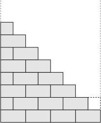
Figure 7: Initial configuration where the component in the kernel of $F$ can be estimated. The dashed brick indicates the only possibility to add a brick.

To use the lemmas above we could use the initial state $a\in\{0,1\}^{ch}$ of the clock which is indicated by the wall in Fig 7. The only possibility to add a brick is at the rightmost position (cell $1,h-1$). Hence $F|a\rangle=(1/\sqrt{2})|a^{\prime}\rangle$ where $a^{\prime}$ is the new wall with the additional half brick. To calculate $F^{\dagger}|a^{\prime}\rangle$ note that $a^{\prime}$ allows only two ways to remove a brick, namely that one just added (then $a^{\prime}$ is mapped to $a$ again) and the upper most brick on the left ($a^{\prime}\mapsto a^{\prime\prime}$). This means that

$$F^{\dagger}F|a\rangle=\frac{1}{2}(|a\rangle\oplus|a^{\prime\prime}\rangle)\,.$$

Hence the angle between $F^{\dagger}F|a\rangle$ and $|a\rangle$ is $\pi/4$. The length of $F^{\dagger}F|a\rangle$ is $L=1/\sqrt{2}$.

Using Lemma 5 we obtain

$$tr(P|a\rangle\langle a|P)\geq\cos^{2}(\pi/4)=1/2\,,$$

and by Lemma 6 we have

$$tr(P_{\delta}|a\rangle\langle a|P_{\delta})\geq\cos^{2}(\pi/4-\arcsin(\sqrt{2}\delta)\,.$$

Note that eigenvalues of $F^{\dagger}F$ of modulus $\delta$ correspond to eigenvalues of $F$ with modulus $\sqrt{\delta}$. If $\tilde{P}_{\epsilon}$ is the spectral projection of $F$ for eigenvalues of at least modulus $\epsilon$ we have

$$tr(\tilde{P}_{\epsilon}|a\rangle\langle a|\tilde{P}_{\epsilon})\geq\cos^{2}(\pi/4-\arcsin(\sqrt{2}\epsilon^{2}))\,.$$

We will use the lemmas in this section to estimate the probability of success of the ergodic quantum algorithm. The idea is as follows. In Section 6 we will argue that the correct result can be found for all states $F^{j}|\psi\rangle$ (where $|\psi\rangle$ is the initial state) for all $j$ satisfying a certain condition. This condition ensures that the circuit $U$ has been applied an odd number of times on the data qubits. To formalize this we introduce spaces ${\cal H}_{l}$ as in lemma 3 which are spanned by the vectors $F^{l+jN}|\psi\rangle$. Let $Q_{l}$ be the projection onto ${\cal H}_{l}$. Then for the probability distribution induced by the time average

$$W(l)=\frac{1}{T}\int_{0}^{T}tr(Q_{l}e^{i-Ht}|\psi\rangle\langle\psi|e^{iHt})\,dt$$

we have a lower bound on each $W(l)$:

Lemma 7

There is an initial state of the clock configuration such that the probability $W(l)$ to find the state in ${\cal H}_{l}$ after one has waited the time $T$ as in lemma 4 is at least

$$W(l)\geq(\frac{1}{N}-2\delta)\cos^{2}(\pi/4-\arcsin(\sqrt{2}\epsilon^{2}))\,.$$

The proof follows immediately from the lemmas of this Section: We choose the initial clock configuration of fig. 7. Above we have argued that the probability for finding a state in the eigenspace with eigenvalues of modulus at least $\epsilon$ is given by the $\cos^{2}$-expression on the right. Given a state in this subspace we have uniform distribution up to a variation distance $\delta$. This yields the factor $1/N-2\delta$.

In the next section we show for which part of the spaces ${\cal H}_{l}$ we have certainly a correct result and how this promise is used in the readout procedure.

6 Initialization and Readout

It is clear that the program qubits have to be initialized according to the simulated quantum circuit. Furthermore we have to initialize all clock qubits. On the data register we have only to initialize those qubits which are located in the cells where the initial clock wave is located.

The readout of the computation result is done as follows. Here we assume that the initial state of the clock register is $|a\rangle$ where all symbols $1$ are in row $0$ (In Section 5 we have also considered another initial configuration which makes is easier to decide which component of the initial state is in the kernel of the Hamiltonian. However, the analysis of this Section is technically more complicated and the output region would have to be enlarged for this initial configuration). We define an output region which consists of all cells with column index between $1$ and $m$ where $m$ is any natural number greater than $2h$.

We choose an arbitrary row in the output region and measure as many clock qubits of this row as are necessary to find the wave front. If we have found a clock qubit in state $|1\rangle$ in position $j,k$ the wave front in row $j+1$ and $j-1$ has to be in one of the columns $k-1$, $k$, or $k+1$. By this procedure we can localize the whole wave front. If it is completely localized in the output region we know that the state of the corresponding logical qubits is either of the states $U(|x\rangle\otimes|0\dots 0\rangle$) or $|x\rangle\otimes|0\dots 0\rangle$. Then we can readout the result. We may define $f$ in such a way that we can decide whether the result is correct or not. In the following we will give a lower bound on the success probability of the whole readout procedure. First we estimate the probability for finding the wave front in the output region.

The wave front starts in row $0$. States in ${\cal H}_{l}$ are in general superpositions of different wave fronts. Note that every such wave front consists of $l\mod g$ bricks. By elementary geometric arguments one can check the following statements: First we consider the case that $l$ is in the interval $0,\dots,g-1$. A wave front which consists of more than $h^{2}/2$ bricks has completely passed row $0$. Similarly, all row indices of the symbols $1$ can be guaranteed to be at most $m$ if $l$ is at most $h(m-h)/2$. Therefore, we have at least $h(m-h)/2-h^{2}/2=h(m-2h)/2$ spaces ${\cal H}_{l}$ which are completely in the output region. We obtain the same number of spaces ${\cal H}_{l}$ for $l=g,\dots,2g-1$. By these arguments we can easily derive the following lower bound. For each space ${\cal H}_{l}$ we can guarantee at least the probability $1/N-2\delta$. This yields the following bound.

Lemma 8 (Probability to find the wave front)

The probability for finding the wavefront completely in the output region is at least

$$h(m-2h)(\frac{1}{N}-2\delta)s_{\epsilon}\,,$$

where $s_{\epsilon}$ is the size of the component of the initial state in the eigenspace of $F$ with eigenvalues of modulus at least $\epsilon$.

However, only the values above in the second interval ensure correct output. Since the function $f$ is without loss of generality $1$ on at least one bit, we can distinguish whether the result has to be rejected and the experiment has to be repeated. The probability that the first experiment succeeds can hence be estimated by dividing the lower bound of Lemma 8 by two:

Theorem 1 (One Shot Success probability)

The probability for finding the output region and furthermore obtaining the correct computation result is at least

$$\frac{h(m-2h)}{2}(\frac{1}{N}-2\delta)s_{\epsilon}\,,$$

with $s_{\epsilon}$ as in Lemma 8.

Note that we have chosen the initial state of Fig. 7 because we were able to prove a lower bound on the length of the component in the image of $F$ which yields a good value for $s_{\epsilon}$. Actually, the disadvantage of this initial state is that the propagation is slow since the wall can grow only at one point. The more natural initial configuration given by a flat wall allows propagation in every second column. For this wall, we do not have a good estimation for the component in the image of $F$ which is as simple as for the wall in Fig. 7. Nevertheless, we believe that it is better to start with the flat wave. If the size of the output region dominates the size of the circuit (i.e. $c\approx m$ and $c\gg h$) the quotient $h(m-2h)/N$ tends to $1$ since $N=c(h+1)$. With small $\epsilon$ the factor in Theorem 1 is almost $1/2$. Hence the success probability tends to $1/4$.

7 Solving PSPACE problems in crystals of polynomial size

It seems to be a general property of our construction that the size of the crystal necessarily grows linearly with the running time (i.e., the depth) of the encoded circuit. From the complexity theoretic point of view, this would have important consequences. Note that the complexity class PSPACE contains all problems which can be solved using polynomial space resources [19]. The running time of an algorithm solving a problem in PSPACE may be exponential. This seems to imply that the ergodic quantum computer would need exponential space in contrast to usual models of computation (e.g. Turing machines and Boolean circuits). Now we want to show briefly that even the ergodic quantum computer can solve all problems in PSPACE in polynomial space.

The key idea is that even if an algorithm has exponential running time, it has necessarily (by definition) a polynomial description of the required sequence of operations. Therefore it is always possible to construct a circuit $U$ of polynomial depth such that the repeated application of $U$ solves the PSPACE problem.

In [20] we have shown that for every problem in PSPACE there is a two-gate quantum circuit $U$ of polynomial size which computes a function $f:\{0,1\}^{n}\rightarrow\{0,1\}^{m}$ in the following sense:

1. There is a (possibly exponentially large) natural number $r$ such that

   $$U^{r}(|x\rangle\otimes|y\rangle\otimes|0\dots,0\rangle)=|x\rangle\otimes|y\oplus f(x)\rangle\otimes|0\dots 0\rangle\,,$$

   where $x\in\{0,1\}^{n}$ is the input string and $y$ is an arbitrary string in the output register.

2. The change of the state of the output register given by

   $$y\mapsto y\oplus f(x)$$

   occurs for a certain power $s$ of $U$, i.e., for all $U^{j}$ with $0\leq j<s$ the output state is still $y$ and for all $U^{j}$ with $s\leq j\leq r-1$ it is already $y\oplus f(x)$.

Furthermore, $r$ and $s$ are known by construction of $U$. This is possible since there is always an upper bound on the running time of an algorithm derived from the restricted space resources. By introducing idle cycles (counting steps) one can guarantee that this bound is exactly attained. Note that it does not make sense to require that the change of the output state occurs during the $r$th application of $U$. Otherwise $f$ could be computed by a single application of $U^{-1}$. This is shown by the following argument:

Assume

$$U^{r}(|x\rangle\otimes|0\dots 0\rangle\otimes|y\rangle)=|x\rangle\otimes|0\dots 0\rangle\otimes|y\oplus f(x)\rangle$$

and

$$U^{r-1}(|x\rangle\otimes|0\dots 0\rangle\otimes|y\rangle)=|\psi\rangle\otimes|y\rangle\,,$$

where $|\psi\rangle$ is an appropriate state of ancilla+input register. Then we have

$$U^{-1}(|x\rangle\otimes|0\dots 0\rangle\otimes|y\oplus f(x)\rangle) = U^{-1}U^{r}(|x\rangle\otimes|0\dots 0\rangle\otimes|y\rangle)$$

$$=|\psi\rangle\otimes|y\rangle$$

This mean that one application of $U^{-1}$ maps $y\oplus f(x)$ onto $y$, i.e., $0$ is mapped onto $f(x)$.

The construction of [20] follows the usual philosophy of reversible computation [21]: The actual computation is done during the first $r/2$ cycles. Then the result is copied to the output register with Controlled-Not gates. The only goal of the last $r/2$ cycles is to undo the computation and restore the initial state.

The ergodic theory in Section 5 applies directly to PSPACE problems after substituting $N=2g$ to $N:=2rg$. Furthermore one has to guarantee the orthogonality condition (11) for all $j\neq k\mod 2rg$. The bit flips which have been explained at the beginning of Section 5 have to be substituted by incrementing counter registers.

The readout is done exactly as in Section 6. Given that we have localized the clock wave front in the output region we have the correct result with probability $1/2$. As in Section 6 we can choose $f$ in such a way that it indicates whether the result has to be rejected. Hence the probability of success is not reduced by the fact that the computation requires more cycles of $U$.

8 Conclusions

We have proposed a model of quantum computing which does not require any control operations during the computation process. The only required operations are the initialization of basis states and the readout in the computational basis.

The relevance of this model is two-fold: first it shows that, in principle, quantum computation can be realized with a small amount of quantum control. Even though our interaction is rather artificially constructed, it is a priori not clear that it is unphysical: It consists of finite range interactions among cells of a crystal which contain some finite dimensional quantum systems. This shows that relatively simple local interactions in homogeneous solid states may have universal power for quantum computing without external control. We admit that it seems difficult to decide whether the interactions in real matter have such properties. However, this may be an interesting question for future research.

The second aim of this paper concerns the thermodynamics of computation. As in [6, 7, 8] the computation is performed in an energetically closed physical system with the additional feature that only the preparation of basis states is required.

It would be desirable to find more simple Hamiltonians which are universal for ergodic quantum computing. A basis to find them could be given by simple $1$-dimensional universal quantum cellular automata.

Acknowledgments

Thanks to Khoder Elzein for drawing the nice cylinders. This work has been supported by grants of the project “Kontinuierliche Modelle der Quanteninformationsverarbeitung” (Landesstiftung Baden-Württemberg).

References

- [1] R. Raussendorf and H. Briegel. Quantum computing via measurements only. (quant-ph/0010033).
- [2] S. Benjamin. Quantum computing with globally controlled exchange-type interactions. quant-ph/0104117.
- [3] S. Benjamin. Schemes for parallel quantum computation without local control of qubits. quant-ph/9909007.
- [4] D. Leung. Two-qubit projective measurements are universal for quantum computation. quant-ph/0111122, 2001.
- [5] D. Aharonov, W. van Dam, J. Kempe, Z. Landau, S. Lloyd, and O. Regev. Adiabatic quantum computation is equivalent to standard quantum computation. quant-ph/0405098, 2004.
- [6] P. Benioff. The computer as a physical system: A microscopic quantum mechanical model of computers as represented by Turing machines. J. Stat. Phys., 22(5), 1980.
- [7] R. Feynman. Quantum mechanical computers. Opt. News, 11, 1985.
- [8] N. Margolus. Quantum computation. Ann. NY. Acad. Sci., 480(480-497), 1986.
- [9] P. Wocjan. Estimating mixing properties of local Hamiltonian dynamics and continuous quantum random walks is PSPACE-hard. quant-ph/0401184.
- [10] A. Kitaev. Quantum measurements and the abelian stabilizer problem. Electronic Colloquium on Computational Complexity, (TR96-003), 1996. see also quant-ph/9511026.
- [11] N. Margolus. Parallel quantum computation. In W. Zurek, editor, Complexity, Entropy, and the Physics of Information. Addison Wesley Longman, 1990.
- [12] A. Yu. Kitaev, A. H. Shen, and M. N. Vyalyi. Classical and Quantum Computation, volume 27 of Graduate Studies in Mathematics. American Mathematical Society, 2002.
- [13] M. Biafore. Can quantum computers have simple Hamiltonians? In Proc. Workshop on Physics of Comp., pages 63–86, Los Alamitos, CA, 1994. IEEE Computer Soc. Press.
- [14] J. Ziman. Principles of the Theory of Solids. Cambridge University Press, 1972.
- [15] N. Margolus. Parallel quantum computation. In W. Zurek, editor, Complexity, entropy, and the physics of information, volume VIII, pages 273–287. Santa Fee Institute, Adison Wesley, 1990. SFI-studies.
- [16] T. Gramss. On the speed of quantum computers with finite size clocks. Santa Fe Institute Working Papers, 1995. http://www.santafe.edu/sfi/publications/wpabstract/199510086.
- [17] D. Aharonov, A. Ambainis, J. Kempe, and U. Vazirani. Quantum Walks On Graphs. Proceedings of ACM Symposium on Theory of Computation (STOC’01), July 2001, p. 50-59.
- [18] P. Diaconis. Group Representations in Probability and Statistics IMS Lecture Notes - Monograph Series, Vol. 11, S. S. Gupta (ed.), Inst. of Math. Stat., Hawyard Ca, 1988.
- [19] Ch. Papadimitriou. Computational Complexity. Addison Wesley, Reading, Massachusetts, 1994.
- [20] P. Wocjan, D. Janzing, Th. Decker, and Th. Beth. Measuring 4-local n-qubit observables could probabilistically solve PSPACE. Proceedings of the WISICT conference, Cancun 2004. quant-ph/0308011.
- [21] C. H. Bennett. Logical reversibility of computation. IBM J. Res. Develop., 17:525–532, 1973.