Communicating continuous quantum variables between different Lorentz frames

Abstract

We show how to communicate Heisenberg-limited continuous (quantum) variables between Alice and Bob in the case where they occupy two inertial reference frames that differ by an unknown Lorentz boost. There are two effects that need to be overcome: the Doppler shift and the absence of synchronized clocks. Furthermore, we show how Alice and Bob can share Doppler-invariant entanglement, and we demonstrate that the protocol is robust under photon loss.

Quantum communication spans a wide range of topics, from cryptography and teleportation, to multi-party entanglement protocols, error correction and purification Bouwmeester et al. (2000). Often, the emphasis is on how we can outperform classical communication protocols with shared entanglement, using only local operations and classical communication. However, we have to be very careful when we consider sharing entanglement, since its distribution is a physical process. As a consequence, it is subject to uncertainties and noise. Moreover, quantum communication protocols typically assume that all parties have perfect knowledge about a global frame of reference. In other words: they all agree on which way they call “up”. Both the distribution and the local (re-) definition of the quantum states needs to be addressed in any practical implementation of the communication protocol.

When Alice and Bob want to establish a (quantum) communication channel, they first need to agree on the specific protocols that they are going to use. As was suggested above, one also might think that they need to share special information such as a (global) fixed frame of reference (see, for example, Ref. Rudolph and Grover (2003) and references therein), or synchronized clocks. However, there are quantum communication protocols that can circumvent the need for, e.g., a global frame of reference Bartlett et al. (2003). On the other hand, establishing perfect clock synchronization has proved much trickier Jozsa et al. (2000); Preskill (2000). The question we address here is whether Alice and Bob can communicate continuous (quantum) variables when they have no prior information about their respective inertial frames of reference. Also, the case for discrete variables was recently proposed Bartlett and Terno (2004).

Such a problem obviously needs to be formulated in a relativistic setting. Recently, there has been considerable interest in relativistic quantum information. It was shown that a fundamental information-theoretic concept such as entropy is not a relativistic scalar Peres et al. (2002) and a Lorentz transformation of subsystems mix the entanglement between spin and momentum Gingrich and Adami (2002). Furthermore, the relativistic transformation of Bell states was derived Alsing and Milburn (2002). In this Letter, we look for invariant quantum states with respect to Lorentz boosts. In addition, we will construct entanglement between the frames of Alice and Bob.

Suppose that Alice and Bob occupy different inertial frames of reference. If they wish to communicate a real number $\lambda$ it is natural to use electromagnetic (quantum) waves, because of its robust properties for long-distance communication. If Alice and Bob do not know their relative velocities, the communication is hampered by two effects: First, any signal sent from Alice to Bob (and vice versa) will suffer from an unknown Doppler shift. Secondly, the local clocks of Alice and Bob will run at different rates to an outside observer. Since many quantum-optical measurements (such as, e.g., homodyne detection) rely intrinsically on timing information, we need to remove the time dependence of the states in the relevant part of the wave function.

The classical way to communicate a real number $\lambda$ is for Alice to send a pulse of coherent light and for Bob to measure the intensity. The Doppler shift only changes the frequency, not the number of photons, so the intensity is invariant. Similarly the time dilation will stretch or compress the pulse, and provided Bob integrates over the whole pulse, he will get the same result. If the coherent amplitude of the pulse is made sufficiently large then the photo-detector will self-homodyne and hence produce a continuous spectrum (corresponding to the in-phase quadrature) on which to encode $\lambda$.

However, coherent light is ultimately shot-noise limited, i.e., we can only estimate $\lambda$ up to a precision $\sqrt{\lambda}$. Secondly, we are interested in the invariant subspaces of continuous quantum-variable systems under Lorentz boosts. The protocol we propose generates these invariant subspaces, and yields Heisenberg-limited precision in determining $\lambda$. Furthermore, we will show that our protocol is robust under photon loss.

Let the four-vector potential of the electromagnetic field be given by

$$A^{\mu}(x)=\int d^{4}k\,\delta(k^{2}-\vec{k}^{2}+k_{0}^{2})\sum_{j}\left[\epsilon_{j}^{\mu}\hat{a}_{j}(k)e^{ikx}+\mathrm{H.c.}\right]\;,$$ (1)

where $k$ and $x$ are the wave and position four vectors, and $\epsilon_{j}$ is the $j$-polarization vector. The frequency of a field mode is given by $k_{0}\equiv\omega_{k}$. Both Alice and Bob describe the field in the Coulomb gauge [$\nabla\cdot\mathbf{A}=0$, with $A^{\mu}=(\phi,\mathbf{A})$], which is not Lorentz invariant. It was shown by Kok and Braunstein Kok and Braunstein (2004) that a pure Lorentz boost $\Lambda$ without rotation does not affect the polarization of the field in the Coulomb gauge, and that the annihilation operator transforms as $\hat{a}_{j}^{\prime}(k)=\sum_{l}U_{jl}\;\hat{a}_{l}(\Lambda k)$ under Lorentz transformations. The $SU(2)$ matrix $U$ corresponds to the overall spatial rotation. Such rotations were considered by Bartlett et al. Bartlett et al. (2003), hence we confine our discussion to pure boosts, yielding $\hat{a}_{j}^{\prime}(k)=\hat{a}_{j}(\Lambda k)$. This allows us to suppress the polarization, and treat the electromagnetic field as a set of scalar fields.

The annihilation operator can be written as

$$\hat{a}(k)=\sqrt{\frac{\omega_{k}}{2\hbar}}\,\hat{q}(k)+\frac{i}{\sqrt{2\hbar\omega_{k}}}\,\hat{p}(k)\;.$$ (2)

Here, $\hat{q}(k)$ and $\hat{p}(k)$ are the (Hermitian) quadratures of the field mode $k$, and they obey the canonical commutation relation $[\hat{q}(k),\hat{p}(k^{\prime})]=i\hbar\,\delta(k-k^{\prime})$. A Doppler shift due to a Lorentz boost $\Lambda$ between inertial frames will result in a transformation $\omega_{k}\rightarrow\mu^{2}\omega_{k}$, where $\mu^{2}=\sqrt{1-\beta^{2}}$. Here, $\beta=v/c$ is Bob’s velocity.

The phase number $kx$ is a scalar (it is the number of wave crests counted by an observer), and therefore invariant under boosts. The modes are thus transformed according to

$$\hat{a}^{\prime}(k)\rightarrow\sqrt{\frac{\omega_{k}^{\prime}}{2\hbar}}\,\hat{q}(\Lambda k)+\frac{i}{\sqrt{2\hbar\omega_{k}^{\prime}}}\,\hat{p}(\Lambda k)\;,$$ (3)

which is equivalent to the transformation

$$\hat{q}(k)\rightarrow\hat{q}^{\prime}(k)=\mu\,\hat{q}(\Lambda k)\quad\text{and}\quad\hat{p}(k)\rightarrow\hat{p}^{\prime}(k)=\frac{1}{\mu}\,\hat{p}(\Lambda k)\;.$$ (4)

A Doppler shift therefore clearly corresponds to a squeezing operation in the phase space $(q,p)$. Indeed, the symmetry group of a quantum oscillator with variable frequency is $SU(1,1)$ Perelomov (1986).

Measuring certain observables of the electromagnetic field often implicitly assumes the existence of a local clock. For example, homodyne detection uses a local oscillator, which serves as the clock. When Alice prepares a state using a local oscillator, there is a priori no reason to believe that Bob’s measurement using a different clock running at a different rate will project onto the same state. The second physical hurdle we have to overcome in communicating continuous variables between different inertial reference frames is therefore to remove the time dependence of the state preparation and measurement stages.

Locally, we can write the time evolution in terms of the following $SU(2)$ quadrature transformation of the field modes:

$$\begin{pmatrix}\hat{q}\\ \hat{p}\end{pmatrix}\rightarrow\begin{pmatrix}\hat{q}^{\prime}\\ \hat{p}^{\prime}\end{pmatrix}=\begin{pmatrix}\cos\phi&\sin\phi\\ -\sin\phi&\cos\phi\end{pmatrix}\begin{pmatrix}\hat{q}\\ \hat{p}\end{pmatrix}\;.$$ (5)

These transformations must leave invariant the part of the quantum state that encodes $\lambda$. However, this does not necessarily mean that the entire quantum state is invariant Knill et al. (2000). Indeed, we will construct invariant states of infinite energy, whose regularized finite-energy states are no longer completely invariant, but retain sufficient invariance to faithfully encode $\lambda$.

The physical motivation for this discussion was that Alice wants to communicate a real number $\lambda$ to Bob, using the quantum properties of light. We can consider two distinct cases of quantum communication of continuous variables. Firstly, we can use quantum states to communicate a classical variable. Secondly, we can communicate a continuous quantum variable, which includes superpositions of real numbers. In the first part of this Letter we consider the first case, and in the second part, we address the latter.

To communicate a real number $\lambda$ with Bob, Alice needs to send a beam or pulse of light in a state $|\lambda\rangle$, such that Bob can retrieve $\lambda$ with some (finite) precision $\Delta\lambda$. In other words, the beam or pulse carrying the information about $\lambda$ must be invariant under Doppler shifts and local time translations. The simplest operator that obeys these requirements is reminiscent of the angular momentum operator $\hat{L}(k)=\hat{q}_{1}(k)\hat{p}_{2}(k)-\hat{p}_{1}(k)\hat{q}_{2}(k)$, where the subscripts on $q$ and $p$ denote two distinct modes (if one uses the polarization degree of freedom to distinguish these modes, then $\hat{L}$ is also invariant under spatial rotations Bartlett et al. (2003)). It exhibits the famous singlet structure of $SU(2)$ representations. Singlets are invariant under unitary transformations of the form $U\otimes U$ (where $U$ is an arbitrary unitary transformation on the subsystem). More importantly, $\hat{L}(k)$ is also invariant under $SU(1,1)$ group transformations, and should therefore be the building block for constructing invariant subspaces (so-called decoherence-free subspaces Zanardi and Rasetti (1997); Lidar et al. (1998)) for continuous-variables quantum communication. We therefore need to construct the eigenstates $|\lambda\rangle$ of $\hat{L}$:

$$\hat{L}(k)|\lambda\rangle=\hat{L}(\Lambda k)|\lambda\rangle=\left(\hat{q}_{1}\hat{p}_{2}-\hat{p}_{1}\hat{q}_{2}\right)|\lambda\rangle=\lambda|\lambda\rangle\;.$$ (6)

From now on, we implicitly assume that $q_{j}$ and $p_{k}$ are labeled by $k$ and $\Lambda k$ for Alice and Bob respectively.

Next, we seek the eigenstates that facilitate the communication of a continuous variable $\lambda$ between Alice and Bob. Define $\psi_{\lambda}(q_{1},q_{2})\equiv\langle q_{1},q_{2}|\lambda\rangle$ as the probability amplitude for the quadrature phases $q_{1}$ and $q_{2}$, and $\hat{p}_{j}=i\hbar\,\partial/\partial q_{j}$. Then the eigen equation is given by

$$i\hbar\left(q_{1}\frac{\partial}{\partial q_{2}}-q_{2}\frac{\partial}{\partial q_{1}}+\frac{i\lambda}{\hbar}\right)\psi_{\lambda}(q_{1},q_{2})=0\;,$$ (7)

which gives us the (unnormalized) state

$$\psi_{\lambda}(q_{1},q_{2})\propto\exp\left[\frac{i\lambda}{\hbar}\arctan\left(\frac{q_{1}}{q_{2}}\right)\right]\,(q_{1}^{2}+q_{2}^{2})\;.$$ (8)

The task is now for Alice to send a state of the form of Eq. (8) to Bob, who can then retrieve the value $\lambda$ by measuring the operator $\hat{L}(\Lambda k)=\hat{q}_{1}\hat{p}_{2}-\hat{p}_{1}\hat{q}_{2}$. However, the state $\psi_{\lambda}(q_{1},q_{2})$ has infinite mean energy, and as a consequence, Alice cannot send this exact state. We can regularize the ‘ideal’ state of Eq. (8) such that they are no longer states with infinite energy (see Fig. 1):

$$\psi_{\lambda}^{a}(q_{1},q_{2})\propto(q_{1}^{2}+q_{2}^{2})e^{\frac{i\lambda}{\hbar}\arctan\left(\frac{q_{1}}{q_{2}}\right)-a(q_{1}^{2}+q_{2}^{2})/2}\;.$$ (9)

The exponential factor $\exp[-a(q_{1}^{2}+q_{2}^{2})/2]$ (with $\mathrm{Re}\,a>0$) ensures that the wave function $\psi_{\lambda}^{a}(q_{1},q_{2})$ remains finite and localized in phase space. Indeed, with the normalization constant $\sqrt{a^{3}/2\pi}$, we find that the mean energy $\langle E\rangle$ of a frequency mode $\omega_{k}$ is

$$\langle E\rangle=\hbar\omega_{k}\left(\frac{1}{2}+\frac{3}{a}\right)\;,$$ (10)

where we used that $E=\hbar\omega_{k}(\hat{n}_{1}+\hat{n}_{2})$, and $\hat{n}_{i}=q_{i}^{2}-\partial^{2}_{q_{i}}$. It is immediately clear that the mean energy diverges only if $a$ becomes zero and $\psi_{\lambda}^{a}$ becomes $\psi_{\lambda}$. For finite $a$ the dispersion in the energy $\Delta E$ is also finite.

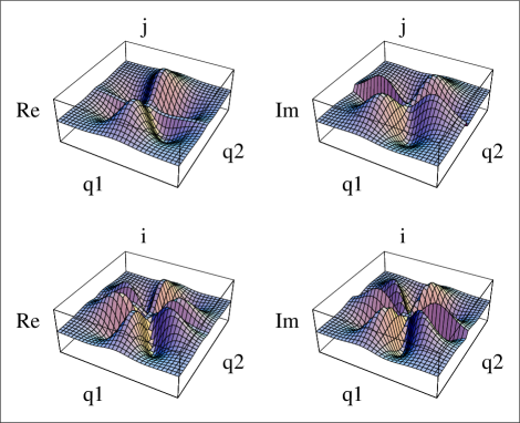
Figure 1: The real and imaginary parts of the probability amplitude for the quadrature phases with finite energy $|\psi_{\lambda}^{a}\rangle$ with $a=1$, $\lambda=3$ and $\lambda=5$ on the interval $-3\leq q_{1},q_{2}\leq 3$.

The state $\psi_{\lambda}^{a}(q_{1},q_{2})$ is not strictly invariant under Lorentz boosts. In particular, a boost parametrized by $\mu$ in Eq. (4) leads to the transformation $a\rightarrow\mu^{2}a$. This corresponds to an expected shape change in the wave packet. However, it is easily shown that Bob’s measurement of the observable $\hat{L}(\Lambda k)$ is not affected by this transformation. When we calculate the expectation values of $\hat{L}(\Lambda k)=q_{1}\partial_{q_{2}}-q_{2}\partial_{q_{1}}$ and $\hat{L}^{2}$, we find that $\langle\hat{L}(\Lambda k)\rangle=\lambda$ and $\langle\hat{L}^{2}(\Lambda k)\rangle=\lambda^{2}+1$. The error in $\lambda$ is then $(\Delta\lambda)^{2}=\langle\hat{L}^{2}\rangle-\langle\hat{L}\rangle^{2}=1$ in units of $\hbar$. That is, Bob can in principle retrieve the value of $\lambda$ by measuring the observable $\hat{L}$ without Alice having to resort to infinite energy states. In practice, Bob will induce an error $\delta\lambda$ associated with his measurement scheme.

Next, we consider what happens when a photon is lost in the process of sending the state $\psi_{\lambda}^{a}$. The loss of a photon is modeled by a beam-splitter $\hat{B}$ with reflection amplitude $\kappa\in\mathbb{R}$, where the reflected beam is traced over. Consequently, $\kappa^{2}$ is the photon loss. When the loss is small, we only need to take into account the first few terms of the unitary evolution $U=\exp[i\kappa\hat{B}]$:

$$\psi_{\lambda,\rm out}^{a}(q_{1},q_{2},q_{3})=\left(1+i\kappa\hat{B}-\frac{\kappa^{2}}{2}\hat{B}^{2}\right)\psi_{\lambda}^{a}(q_{1},q_{2})\;.$$

In the Bargmann representation, we have $\hat{B}=iq_{3}\partial_{q_{1}}-iq_{1}\partial_{q_{3}}$. When we collect terms up to $\kappa^{2}$, the expectation value of an observable $\hat{A}$ in the presence of the loss mechanism is given by

$$\langle\hat{A}\rangle_{B} = \langle\hat{A}\rangle+\kappa^{2}\int dv\,\bar{\psi}_{\lambda}^{a}\hat{B}^{\dagger}\hat{A}\hat{B}\,\psi_{\lambda}^{a}$$ (12)

$$+\frac{\kappa^{2}}{2}\int dv\,\bar{\psi}_{\lambda}^{a}(\hat{B}^{\dagger 2}\hat{A}+\hat{A}\hat{B}^{2})\,\psi_{\lambda}^{a}\;,$$

where the integral $\int dv=\iiint dq_{1}\,dq_{2}\,dq_{3}$, and $\bar{\psi}$ denotes the complex conjugate.

When we calculate $\langle\hat{L}\rangle_{B}$ and $\langle\hat{L}^{2}\rangle_{B}$, we find

$$\langle\hat{L}\rangle_{B}=\lambda\qquad\text{and}\qquad\Delta L_{B}\simeq 1+\frac{a\kappa^{2}}{12}(2+\lambda^{2})\;.$$ (13)

The expectation value $\langle\hat{L}\rangle_{B}=\langle\hat{L}\rangle$ is not affected, while the precision $\Delta L_{B}$ starts to deteriorate when $\lambda$ becomes too large. However, this can be made arbitrarily small by reducing $a$. The ideal infinite-energy states ($a\rightarrow 0$) do not suffer from reduced precision at all.

The states in Eqs. (8) and (9) are in some sense “ideal” choices, but at this point we have no idea how to produce these states. Furthermore, they are by no means the only choice. Any polynomial operator $\hat{A}=\hat{A}(\hat{L})$ that has sufficient structure to encode $\lambda$ must be invariant under the quadrature transformations of Eq. (5), and the eigenstates of $\hat{A}$ are therefore suitable for our purposes: $\hat{A}(\hat{L})\,|\Phi_{\alpha}\rangle=\alpha(\lambda)\,|\Phi_{\alpha}\rangle$, where $\alpha(\lambda)$ is a bijective function of $\lambda$. The set of all operators $\hat{A}$ with their associated detection of $\alpha(\lambda)$ determine a class of possible protocols to communicate between different inertial reference frames. An important operator of this type is given by $\hat{A}=\exp[i\lambda(\hat{q}_{1}\hat{p}_{2}-\hat{q}_{2}\hat{p}_{1})]$. This operator can in principle be generated with parametric down-conversion, and it opens a gateway to the practical implementation of this protocol. To this end, we need to find optimal ways to estimate $\lambda$ Bollini and Oxman (1993); Milburn et al. (1994).

In the remainder of this Letter, we consider superpositions of the form $\int d\lambda f(\lambda)|\lambda\rangle$, where $\int d\lambda|f(\lambda)|^{2}=1$. Since Lorentz transformations are unitary, these superpositions remain coherent when sent to Bob. However, the superposition might change due to the Lorentz transformation.

Consider $\hat{L}$ as the generator of a symmetry group parametrized by a conjugate variable $\beta$: $|\psi(\beta+d\beta)\rangle=\exp(id\beta\hat{L}/\hbar)|\psi(\beta)\rangle$. Using a Taylor expansion in $\beta$, we find

$$i\hbar\frac{d}{d\beta}|\psi(\beta)\rangle=\hat{L}|\psi(\beta)\rangle\;,$$ (14)

or $|\psi(\beta)\rangle=\exp(i\beta\hat{L}/\hbar)|\psi\rangle$. In the interaction picture, we write $|\psi\rangle$ independent of $\beta$, and an operator $\hat{A}$ evolves according to $\exp(i\beta\hat{L}/\hbar)\hat{A}\exp(-i\beta\hat{L}/\hbar)$.

General superpositions of $|\lambda\rangle$ then evolve according to

$$\int d\lambda f(\lambda)|\lambda\rangle~{}\rightarrow~{}\int d\lambda f(\lambda)e^{-i\lambda\beta/\hbar}|\lambda\rangle\;.$$ (15)

Given a suitable superposition, Alice and Bob can determine $\beta$ with (possibly Heisenberg limited) precision. Alternatively, Alice can send four-mode superpositions of the form

$$\int d\lambda f(\lambda)|\Phi_{\lambda}\rangle\equiv\int d\lambda f(\lambda)|\lambda,-\lambda\rangle\;,$$ (16)

which are manifestly invariant under $\beta\rightarrow\beta^{\prime}$. We can now build entangled states that are invariant under Lorentz transformations:

$$|\Upsilon\rangle_{AB}=\int d\lambda f(\lambda)\,|\Phi_{\lambda}\rangle_{A}|\Phi_{\lambda}\rangle_{B}\;.$$ (17)

A complete set of continuous-variable “Bell”-states is then given by $\int d\lambda\,g(\lambda,\zeta)\,|\Phi_{\lambda}\rangle_{A}|\Phi_{\lambda\oplus\zeta}\rangle_{B}$ Braunstein (1998), where $\zeta\in\mathbb{R}$, and the subscripts $A$ and $B$ denote the modes held by Alice and Bob respectively. At this point, we should note that we can no longer use the polarization degree of freedom alone to distinguish between $q_{j}$ and $q_{k}$. However, we can use a specific color ordering, since Doppler shifts do not change the order of the spectrum.

In conclusion, we have constructed a class of finite energy states of the electromagnetic field that can be used to send continuous quantum variables from one Lorentz frame to another without knowledge of their relative velocity. These states are therefore invariant under Doppler shifts. Also, the wave function needs to have a time-independent component since time dilatation prevents Alice and Bob from having synchronized local oscillators. We found a multi-mode operator that may serve as a natural building block to construct invariant subspaces under Lorentz transformations over continuous variables. This protocol can also be used by Alice and Bob to share continuous-variable entanglement. Furthermore, the states are robust under small photon loss.

P.K. wishes to thank Sam Braunstein and Bill Munro for valuable comments. Part of the research described in this Letter was carried out at the Jet Propulsion Laboratory, California Institute of Technology, under a contract with the National Aeronautics and Space Administration (NASA). P.K. was supported by the United States National Research Council, the Australian Centre for Quantum Computer Technology, and the European Union RAMBOQ project.

References

- Bouwmeester et al. (2000) D. Bouwmeester, A. Ekert, and A. Zeilinger, The Physics of Quantum Information (Springer-Verlag Berlin Heidelberg, 2000).
- Rudolph and Grover (2003) T. Rudolph and L. Grover, Phys. Rev. Lett. 91, 217905 (2003).
- Bartlett et al. (2003) S. D. Bartlett, T. Rudolph, and R. W. Spekkens, Phys. Rev. Lett. 91, 027901 (2003).
- Jozsa et al. (2000) R. Jozsa, D. S. Abrams, C. P. Williams, and J. P. Dowling, Phys. Rev. Lett. 85, 2010 (2000).
- Preskill (2000) J. Preskill, quant-ph/0010098 (2000).
- Bartlett and Terno (2004) S. D. Bartlett and D. R. Terno, quant-ph/0403014 (2004).
- Peres et al. (2002) A. Peres, P. F. Scudo, and D. R. Terno, Phys. Rev. Lett. 88, 230402 (2002).
- Gingrich and Adami (2002) R. M. Gingrich and C. Adami, Phys. Rev. Lett. 89, 270402 (2002).
- Alsing and Milburn (2002) P. M. Alsing and G. J. Milburn, Quant. Inf. Comput. 2, 487 (2002).
- Kok and Braunstein (2004) P. Kok and S. L. Braunstein, quant-ph/0407259 (2004).
- Perelomov (1986) A. M. Perelomov, Generalized coherent states (Springer Verlag, 1986).
- Knill et al. (2000) E. Knill, R. Laflamme, and L. Viola, Phys. Rev. Lett. 84, 2525 (2000).
- Zanardi and Rasetti (1997) P. Zanardi and M. Rasetti, Phys. Rev. Lett. 79, 3306 (1997).
- Lidar et al. (1998) D. A. Lidar, I. L. Chuang, and K. B. Whaley, Phys. Rev. Lett. 81, 2549 (1998).
- Bollini and Oxman (1993) C. G. Bollini and L. E. Oxman, Phys. Rev. A 47, 2339 (1993).
- Milburn et al. (1994) G. J. Milburn, W.-Y. Chen, and K. R. Jones, Phys. Rev. A 50, 801 (1994).
- Braunstein (1998) S. L. Braunstein, Nature 394, 47 (1998).